Joint Bilateral Filter for Signal Recovery from Phase Preserved Curvelet Coefficients for Image Denoising

Abstract

Thresholding of Curvelet Coefficients, for image denoising, drains out subtle signal component in noise subspace. This produces ringing artifacts near edges and granular effect in the denoised image. We found the noise sensitivity of Curvelet phases – in contrast to their magnitude – reduces with higher noise level. Thus, we preserved the phase of the coefficients below threshold at coarser scale and estimated their magnitude by Joint Bilateral Filtering (JBF) technique from the thresholded and noisy coefficients. In the finest scale, we apply Bilateral Filter (BF) to keep edge information. Further, the Guided Image Filter (GIF) is applied on the reconstructed image to localize the edges and to preserve the small image details and textures. The lower noise sensitivity of Curvelet phase at higher noise strength accelerate the performance of proposed method over several state-of-the-art techniques and provides comparable outcome at lower noise levels.

I Introduction

Digital image is corrupted during acquisition, transmission and reception systems by different noises. The resultant noise due various sources in these situations can be modeled as additive Gaussian noise (AWGN). Thus the noisy image $y$ may be represented as follows:

$$y(\mathcal{P})=z(\mathcal{P})+\eta(\mathcal{P})$$ (1)

Where, the latent image, $z(\mathcal{P})$ is contaminated with uncorrelated, zero mean additive white Gaussian noise (AWGN), $\eta\in\aleph({0,{\sigma}^{2}})$ to produce noisy image $y(\mathcal{P})$ on a $2D$ grid of $\mathcal{P}\in{\mathbb{R}}^{2}$. Out of several attempts to recover the latent image, ‘Sparse-Land’ signal modeling and non-local (and/or local) patch based image synthesis in spatial domain are proved to be most powerful tools.

In ‘Sparse-Land’ modeling, an image is represented with minimum number of non-zero coefficients (sparse) in multiple scales. Thus a well estimated threshold – at different scales, $\gamma$ – may be able to separate signal from noise subspace by keeping coefficients of higher magnitude. The thresholded coefficients ($\hat{Y}_{\gamma}$) is transformed back into spatial domain to produce the denoised image, $\hat{z}(\mathcal{P})$ as formulated in Eq.2.

$$Y_{\gamma} =\mathcal{\textbf{T}}_{\gamma}\left[y(\mathcal{P})\right]$$ (2a)

$$\hat{Y}_{\gamma} =\begin{cases}Y_{\gamma}~{},&\text{if\, $|Y_{\gamma}|>{\lambda_{\gamma}}$}\\ 0~{},&\text{otherwise}\end{cases}$$ (2b)

$$\hat{z}(\mathcal{P}) =\mathcal{\textbf{T}}_{\gamma}^{-1}\left[\hat{Y_{\gamma}}\right]$$ (2c)

Among a number of image transformation techniques, researchers had used redundant or non-redundant wavelet dictionaries for denoising and kept the salient image features like edges [1, 2, 3, 4, 5, 6, 7, 8, 9, 10]. Recently, Curvelet transform is observed to represent images with edges, even more sparsely [11, 12, 13, 14]. In this technique, an image is decomposed into magnitude and phase at multiple scales and directions. A hard threshold based approach was reported in [11] to separate the signal from the noise subspace. Here, the threshold is computed from and applied to the magnitude of the Curvelet coefficients to recover the signal from the noisy observation. This removes the corresponding phases too. Moreover, portions of the signal components may spilled into noise subspace and are lost. The hard thresholding also introduces ringing artifacts around the edges due to sudden jump in coefficient magnitudes. At the finest scale signal and noise magnitudes are comparable. Therefore, removal of coefficients with thresholds introduces granular artifacts in the denoised image.

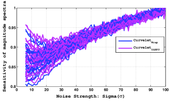
(a)

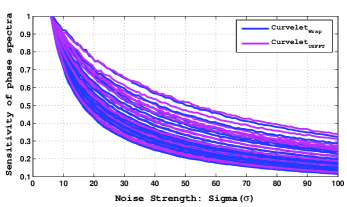
(b)

Figure 1: Noise sensitivity (Normalized between $[0,1]$) of (a) Magnitude & (b) Phase for Curvelet Transform – Wrapping and USFFT – on the images of TID$2008$ Database [15].

Unlike frequency domain approaches, modern spatial filters extract self similarities among local or non-local regions for denoising [16, 17, 18, 19]. Among these methods, Bilateral Filter [16] and its variants [20] – while retain edges effectively – fail to restore smooth regions . This low contrast region can be recovered by determining the chromatic distance of bilateral filter from additional image different from the image of concern. This leads to Joint Bilateral Filter for image restoration [21].

Recently, several methods utilized the advantages of one domain to improve the denoising performance in another domain [22, 23, 24, 25]. Multiresolution Bilateral Filter (MBF) implements BF in the approximation scales to suppress the coarser-grain (low frequency) noise and thresholds the wavelet coefficients in detail scales to remove the fine-grain (high frequency) noise [22]. Similar to MBF, DDID [26] integrated Joint Bilateral Filter (JBF) and Short Time Fourier Transform (STFT) based wavelet shrinkage technique for image denoising. Furthermore, Kumar et al. [27] applied wavelet thresholding to recover the lost image detail from the residual image of NLM filter. The inability of wavelets in handling curve singularity may limit the performance of these hybrid techniques. The Non Subsampled Shearlet Transform (NSST) – in contrast to wavelet – represents image along multiple directions [28]. A linear combination of local Wiener filter and its method noise thresholded image using NSST is proposed in [25] to recover the image from its noisy observation. However the selection of parameters for linear combination in [25] is intuitive, which may limit its performance for wide variety of natural images. In contrast with several variants of combined approaches, block matching 3D collaborative filtering (BM3D) technique excelled in denoising by grouping the similar (non-local) patches and collaboratively filtering the 3D blocks using 1D wavelet thresholding [29]. The state-of-the-art BM3D technique still inadequate in restoring few homogenous regions that manifests as low-frequency noise [30].

We found the noise sensitivity of Curvelet phase – in contrast to its magnitude – reduces with higher noise level. This indicates preserving the phase of Curvelet coefficients may improve denoising quality. We (re)estimated the signal magnitude in the coarser scales by implementing JBF on the thresholded coefficients. This process recovers the signal residuals from the noise subspace, while retaining the indispensable phase information. On the other hand, the implementation (fast) BF (using Fourier kernels [31]) in the finest scale ensures the elimination of granular artifacts with well-connected edges in the restored image. Finally, the reconstructed image is further processed using GIF ($\mathcal{O}(M)$) for better preservation of local structures like: edges, textures and small details. The performance of the proposed algorithm is measured using a few statistical and edge localization measures to compare its efficacy with several state-of-the-art techniques.

The rest of the article is organized as follows: Section II provides few justification on the use of JBF and BF in Curvelet domain and also illustrates the noise sensitivity of the phase and the magnitude under additive Gaussian noise (AWGN). The proposed method for image denoising is explained in Section III. The experimental results are given and discussed in Section IV. Finally, Section V concludes the paper.

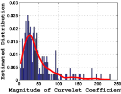
(a)

(b)

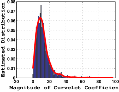
(c)

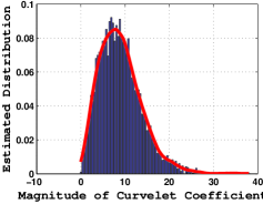
(d)

Figure 2: Estimated distribution (PDF) of noisy image (contaminated with AWGN $\sigma=25$) Curvelet coefficients at (a) scale, $\gamma=2$ & orientation $o=2$; (b) scale, $\gamma=3$, orientation $o=3$; (c) scale, $\gamma=4$, orientation $o=4$; (d) scale, $\gamma=5$, orientation $o=5$.

II Noise Analysis in Curvelet Domain

Curvelet transform decomposes the pixel energy into magnitude and phase components. Literature indicates that the phases of any complex signal transform retain more structural information and are less sensitive to additive Gaussian noise compared to their magnitude [32, 33, 34]. Assuming, that the Curvelet uses tight frames to represent any square integral function $f$ then it must obey Parseval’s identity as [13]:

$$f=\sum_{\gamma,\tau,o}{\langle f,\phi_{\gamma,\tau,o}\rangle}\phi_{\gamma,\tau,o}$$ (3)

Panigrahi et al. [34] utilized the linearity property of Curvelet to derive the sensitivity of magnitude, $\frac{\partial|Y|}{{\partial}{|N|}}$ and phase, $\frac{\partial{\varphi_{Y}}}{{\partial}{|N|}}$ as:

$$\frac{\partial|Y|}{{\partial}{|N|}}=\frac{|N|+|Z|cos(\varphi_{Z}-\varphi_{N})}{\left(|Z|^{2}+|N|^{2}+2|Z||N|cos(\varphi_{Z}-\varphi_{N})\right)^{1/2}}$$ (4)

$$\frac{\partial{\varphi_{Y}}}{{\partial}{|N|}}=\frac{|Z|sin(\varphi_{N}-\varphi_{Z})}{|Z|^{2}+|N|^{2}+2|Z||N|cos(\varphi_{Z}-\varphi_{N})}$$ (5)

where, $\varphi_{Z}$ and $\varphi_{N}$ are the phase angles of the latent image, $z$ and noise, $\eta$ respectively. For experimental validation, we defined noise sensitivity as the ratio of difference between the magnitudes (or phase) of noisy curvelet coefficients to that of magnitude difference between the coefficients of AWGN for consecutive noise levels. The average of this measure is normalized between $[0,1]$ for $\sigma=[5,100]$. The sensitivity measure of curvelet magnitude and phase for each reference image of TID$2008$ database [15] contaminated with AWGN are shown in Fig.1a and 1b, respectively. It indicates that the rate of change of Curvelet phase is less corrupted by AWGN compared to its magnitude. This justifies the preservation of phase in noise subspace, while estimating signal residuals using JBF.

The estimated PDF of Curvelet coefficients of a noisy image at different scales and orientations is shown in Fig.2. It can be observed that the anisotropic scaling of Curvelet transform shapes the PDF of its magnitude at any scale ($\gamma$) and orientation ($o$) to leptokurtic i.e. very sharp peak at zero amplitude and extended tail on the either sides [35, 36]. However, the threshold in [11] is estimated by assuming Gaussian distribution of the curvelet coefficients [36]. The imprecise assumption in Curvelet thresholding leaves a few portions of the signal components in the noise subspace. We then re-estimate the thresholded coefficients to recover the suppressed signal in noise subspace using JBF. The current approach also aides in preserving the corresponding phase information that may strengthen the edges of denoised image.

Figure 3: Solution Approach to the Proposed Problem Definition.

III Proposed Image Denoising Framework

In contrast to the Curvelet thresholding (CT) approach in Eq.2, the proposed formulation in Eq.6 preserves the signal components in the coarser scales, if the coefficients, $C\geq\lambda_{\gamma}$. The spilled or residual signals in the noise subspace (for $C<\lambda_{\gamma}$) are estimated using multiscale Joint Bilateral Filter (JBF), $\boldsymbol{\mathrm{A}_{JBF,C<\lambda_{\gamma}}}$. On the other hand the high frequency components such as: edges, textures and small details in the finest scale are retained maximally using Bilateral Filter, $\boldsymbol{\mathrm{A}_{BF,\gamma}}$. In the proposed formulation the parameters (of different filters in Curvelet domain) are optimized by minimizing the mean square error (MSE) $\boldsymbol{\|E_{\gamma}\|}$ between the estimated and the desired coefficients, assuming obtained by using the operator, $\boldsymbol{\mathrm{B}_{\gamma}}$. Further, the post-processing Guided Image Filter (GIF), $\boldsymbol{\mathrm{C}_{GIF}}$ in the spatial domain is adopted for better localization and preservation of local image structures like: edges, textures and small details.

$$\centering\boldsymbol{\mathrm{A}_{\gamma}}=\left[\boldsymbol{\overline{\mathbf{I}}_{C\geq\lambda_{\gamma}}}\mid\boldsymbol{\mathrm{A}_{JBF,C<\lambda_{\gamma}}}\mid\boldsymbol{\mathrm{A}_{BF,\gamma}}\right]\@add@centering$$ (6)

The various steps involved in the proposed multiscale framework is illustrated in Fig.4. The JBF followed by hard thresholding in the coarser scales is used to recover the lost signal in noise subspace. In the finest scale, BF ensures the preservation of well connected edges. However, the inevitable ringing artifacts in the reconstructed image requires further processing. We applied guided image filter (GIF) in the reconstructed image to localize the edges and to preserve the small details and textures of the latent image, maximally. The complete description and formulation involved in each step of the proposed image denoising technique are discussed in the following subsections.

Figure 4: Illustration of various steps involved in the proposed image denoising framework.

III-A Recovering Signal from Noise Subspace using JBF

Redefining Eq.2b, for curvelet transform and assuming $Y_{\gamma,o}$ as the noisy coefficients at any (coarser) scale $\gamma$ and orientation $o$, the thresholded coefficient is obtained as [11]:

TABLE I: Average Correlation Coefficient between the Estimated coefficient in noise subspace —using both Curvelet hard thresholding (CT(Hard)) [11] and Proposed method— and Original Curvelet Coefficient at different Coarser Scales on TID$2008$ Image Database [15].

Noise Strength	$\gamma=2$		$\gamma=3$		$\gamma=4$		$\gamma=5$
	CT (Hard)	Proposed	CT (Hard)	Proposed	CT (Hard)	Proposed	CT (Hard)	Proposed
$\sigma=10$	0.9932	0.9956	0.9439	0.9798	0.7910	0.9249	0.4681	0.7396
$\sigma=20$	0.9737	0.9877	0.8508	0.9476	0.5723	0.8066	0.2388	0.5366
$\sigma=25$	0.9609	0.9815	0.7985	0.9257	0.4835	0.7463	0.1755	0.4629
$\sigma=30$	0.9463	0.9741	0.7454	0.9017	0.4071	0.6881	0.1320	0.4027
$\sigma=40$	0.9130	0.9536	0.6479	0.8541	0.2916	0.6136	0.0799	0.3494
$\sigma=50$	0.8737	0.9370	0.5600	0.8105	0.2162	0.5310	0.0520	0.2986
$\sigma=75$	0.7636	0.8839	0.3892	0.6963	0.1177	0.3795	0.0231	0.2245

$$\centering Y_{\gamma,o}^{\prime}=\begin{cases}Y_{\gamma,o}~{},&\text{if\, $|Y_{\gamma,o}|>{\lambda_{\gamma},o}$}\\ 0~{},&\text{otherwise}\end{cases}\@add@centering$$ (7)

where, the threshold, $\lambda_{\gamma,o}$ is defined as:

$$\centering T_{\gamma,o}={k}{\sigma}{\sigma_{\gamma,o}}\@add@centering$$ (8)

Here, $k$ is assumed to be a scale dependant constant and $\sigma_{\gamma,o}$ is estimated using Monte Carlo simulation of the Curvelet transform of a few standard white noise images [11].

The initial estimate $Y_{\gamma,o}^{\prime}$ introduces ringing artifacts and looses phase information due to thresholding. The thresholded coefficients in Eq.7 is further processed using JBF [21] to recover the lost signal from the noise subspace (below threshold) as:

$$\tilde{Y}_{\gamma,o}(U)=\frac{1}{C^{c}}\sum_{r\in\aleph_{JBF}(U)}e^{-\frac{{\|r-U\|}^{2}}{2\left(\sigma_{d}^{c}\right)^{2}}}e^{-\frac{{\|Y_{\gamma,o}(r)-Y_{\gamma,o}(U)\|}^{2}}{2\left(\sigma_{r}^{c}\right)^{2}}}Y_{\gamma,o}^{\prime}(r)$$ (9)

where, $\aleph_{JBF}(U)$ is the spatial neighboring window (in Curvelet domain) around $U$. The normalizing constant $C^{c}$ ensures the coefficient weights sum must converge to $1.0$. The parameters, $\sigma_{d}^{c}$ and $\sigma_{r}^{c}$ are the standard deviations of the exponential functions defined for spatial and photometric distances, respectively. The photometric distance parameter is selected as $\alpha$ times of the total range of coefficient magnitude.

The justification of JBF to extract information from below threshold is empirically examined over the Curvelet hard thresholding technique [11]. The original Curvelet coefficient and estimated coefficients using both Curvelet hard thresholding and proposed method in coarser scales are calculated for different noise strength $\sigma$ on TID2008 image database. Table.I indicates that the estimated coefficients in noise subspace are highly correlated with original Curvelet coefficient. Therefore the proposed estimation of signal in noise subspace suppresses noise and retains better interdependency among the coefficients at different scales. Since the phase is indispensable for image representation [33] and it is also less corrupted compared to the Curvelet magnitude, thus we retain the corresponding phase of estimated magnitude in noise subspace.

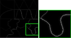
(a)

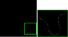
(b)

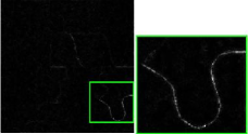
(c)

Figure 5: Curvelet coefficients in the fine scale for (a) Original Texture image and the recovered details from the AWGN of $\sigma=25$ using (b) Curvelet Thresholding and (c) Bilateral filtering.

III-B Retaining Small Details using BF

High frequency components such as: edges, textures and small details are captured by the coefficients in the finest scale. It is observed that few signal and noise magnitudes in this scale are comparable. The application of hard threshold removes both noise and a part of these details resulting in granular effect – due to discontinuous edges as shown in Fig.5b – in the restored image. Thus, Unlike [11], we have computed the denoised coefficients in the finest scale, $\gamma$ using BF [16]:

$$\tilde{Y}_{\gamma}(U)=\frac{1}{C^{f}}\sum_{r\in\aleph_{BF}(U)}e^{-\frac{{\|r-U\|}^{2}}{2\left(\sigma_{d}^{f}\right)^{2}}}e^{-\frac{{\|Y_{\gamma}(r)-Y_{\gamma}(U)\|}^{2}}{2\left(\sigma_{r}^{f}\right)^{2}}}{Y}_{\gamma}(r)$$ (10)

Similar to the Eq.9, the falling rate parameters of the BF kernels in spatial and intensity domain is defined as $\sigma_{d}^{f}$ and $\sigma_{r}^{f}=k_{r}\times\lambda_{\gamma}$, respectively. As illustrated in Fig.5 the filtered output in the finest scale removes the granular effect, while preserving the well-connected edges compared to thresholding [11].

III-C Post Processing using GIF

Though the estimation of signal – in coarser scale – below threshold attenuates the sudden jumps in coefficient magnitude, still requires further processing to remove the ringing artifacts in the reconstructed image. The fast ($\mathcal{O}(M)$) “Edge-Aware" Guided Image Filter (GIF) is considered here to suppress the distortions around the edges of the reconstructed image, $\tilde{z}$. In the absence of guidance image $G$, it is assumed that $G\equiv\tilde{z}$ and the GIF is reformulated as [37]:

$$\hat{z}(\mathcal{P})=\bar{a}_{\mathcal{P}}\tilde{z}(\mathcal{P})+\bar{b}_{\mathcal{P}}$$ (11)

where,
$\bar{a}_{\mathcal{P}}=\frac{1}{|\aleph_{GIF}(\mathcal{P}^{\prime})|}\sum_{{\mathcal{P}^{\prime}}\in\aleph_{GIF}(\mathcal{P})}a_{\mathcal{P}^{\prime}}$
& $\bar{b}_{\mathcal{P}}=\frac{1}{|\aleph_{GIF}(\mathcal{P}^{\prime})|}\sum_{{\mathcal{P}^{\prime}}\in\aleph_{GIF}(\mathcal{P})}b_{\mathcal{P}^{\prime}}$ are the average values of $a_{\mathcal{P}^{\prime}}$ and $b_{\mathcal{P}^{\prime}}$ for all the overlapping windows that covers the pixel $\mathcal{P}$. The linear parameters, $a_{\mathcal{P}^{\prime}}$ and $b_{\mathcal{P}^{\prime}}$ that ensures the preservation edges are estimated as:

$$a_{\mathcal{P}^{\prime}} =\frac{\sigma_{\tilde{z}}^{2}(\mathcal{P}^{\prime})}{\sigma_{\tilde{z}}^{2}(\mathcal{P}^{\prime})+\epsilon}$$ (12a)

$$b_{\mathcal{P}^{\prime}} =(1-{a}_{\mathcal{P}^{\prime}}){\mu}_{\tilde{z}}(\mathcal{P}^{\prime})$$ (12b)

The regularization parameter $\epsilon=k_{1}\times\sigma$ penalizes the over smoothing of edges. The significance of the application of GIF can be observed in Fig.6. Both the visual and quantitative improvement in terms of PSNR and SSIM [38] measure demonstrate its efficacy in preserving small details, while suppressing the distortion around the edge.

(a)

(b)

Figure 6: Proposed denoised method for Lena image ($\sigma$ = 40), (a) Before (PSNR = 29.4091, SSIM = 0.8254) and (b) After (PSNR = 30.001, SSIM = 0.8620) application of GIF.

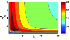
(a)

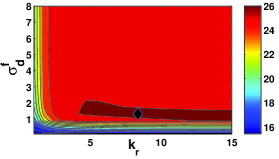
(b)

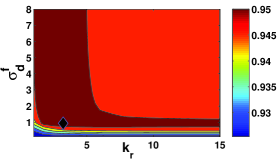
(c)

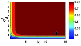
(d)

Figure 7: Tuning of BF parameters, $\sigma_{d}^{f}$ and $k_{r}$ to obtain maximum denoising performance. The mean PSNR measure at different values of $\sigma_{d}^{f}$ and $k_{r}$, when image is contaminated with AWGN of (a) $\sigma=10$ and (b) $\sigma=50$. Similarly, the SSIM measures is also obtained for image corrupted with AWGN of (c) $\sigma=10$ and (d) $\sigma=50$. The “black diamond" symbol indicates peak value. The experiment was conducted on the reference images of TID2008 database [15]

IV Experimental Results & Discussion

Most of the literatures are confined in using a particular type of image sets for the analysis of corresponding denoising algorithm/s [39]. Moreover, the image quality assessment (IQA) measures such as: Peak Signal to Noise Ratio (PSNR) and Structural Similarity Index Measure (SSIM) [38] may not completely evaluate the performance of several image denoising techniques [40, 41]. Therefore, for completeness, in addition to the PSNR and SSIM indices, authors have considered the edge keeping index (EKI) to measure the edge strength (in terms of its magnitude) retained by the denoised image $\hat{z}$ compared to its true edges in $z$ as [42]:

$$EKI=\frac{\sum\limits_{\mathcal{P}=1}^{M}\left[\Delta z(\mathcal{P})-\Delta\mu_{z}\right]\left[\Delta\hat{z}(\mathcal{P})-\Delta\mu_{\hat{z}}\right]}{\sqrt{\sum\limits_{\mathcal{P}=1}^{M}\left[\Delta z(\mathcal{P})-\Delta\mu_{z}\right]^{2}\sum\limits_{\mathcal{P}=1}^{M}\left[\Delta\hat{z}(\mathcal{P})-\Delta\mu_{\hat{z}}\right]^{2}}}$$ (13)

where, the reference image, $z$ and the denoised image, $\hat{z}$ are passed though high-pass filter (viz. Laplacian operator) to obtain $\Delta z$ and $\Delta\hat{z}$, respectively. Moreover, $\Delta\mu_{z}$ and $\Delta\mu_{\hat{z}}$ represent the mean of filtered output of original and restored image. A higher value of EKI – in an interval $[0,1]$ – indicates that the edge strength of original image is well preserved by the denoised image. In the following subsections, few parameters of the proposed algorithm is tuned empirically using above image quality assessment (IQA) indices for a wide variety of natural images, before accessing its performance, quantitatively.

IV-A Parameter Optimization

The performance of proposed image denoising algorithm depends on the selection of both spatial and intensity domain parameters of JBF and BF in the coarser and the finest scale. The weights of the BF (and JBF) are multiplied and if one of the weights closes to zero, then no smoothing occurs. Thus choosing a narrower spatial kernel with larger range kernel produces limited smoothing. The dependencies among the kernels require combined tuning of $\alpha$ and $\sigma_{d}^{c}$ in the coarser scales for JBF (see Eq.9) and $k_{r}$ and $\sigma_{d}^{f}$ in the finest scale for BF (see Eq.10). We experimentally tuned these parameters in terms of maximum PSNR and SSIM measures at low ($\sigma=10$) and high ($\sigma=50$) noise levels, assuming the other parameters as given in Table.II are constant. The tuning of $\sigma_{d}^{f}$ and $k_{r}$ is shown in Fig.7 for TID2008 image database [15]. It may be observed that the optimal value of $\sigma_{d}^{f}$ is relatively independent to the noise variance $\sigma$ compared to $k_{r}$. On the other hand, the parameter $k_{r}$ changes significantly with $\sigma$. At lower noise strength $\sigma=10$ (see Fig.7a), when $k_{r}$ is sufficiently large, increasing the spatial kernel parameter $\sigma_{d}$ over-smooth the coefficients. However, at higher noise strength $\sigma=50$, when $k_{r}$ occupies larger value, the range kernel widens and flattens i.e. it becomes nearly constant over the intensity interval of the noisy coefficient. Therefore at higher $\sigma$ the change in denoising quality is insignificant with further change in $k_{r}$.

Literature suggests theoretically, it is difficult to select a single value of, $\sigma_{r}/\sigma$ (both in case of JBF and BF), which is optimal for all images and $\sigma_{d}$ value [22]. However, based on experimental observation, we fixed a single value for $\sigma_{d}$ for all noise levels. On the other hand, the range parameter, $\sigma_{r}$ is selected according to the noise strength $\sigma$. Unlike, JBF and BF, the parameters $k$ and $k_{1}$ in Eq.8 and Eq.12 are tuned independently to obtain maximum denoising quality. The final optimized values of these parameters are given in Table.II. In this article, the proposed image denoising technique is quantified and compared with several state-of-the-art techniques considering the default parameter values as given in Table.II.

TABLE II: Optimized Parameter Values for Proposed Image Denoising Framework.

Parameters	Symbol	Default Values
Thresholding Parameter	$k$	2.0
JBF Kernels Shape Control Parameters	$\alpha$	0.04
	$\sigma_{d}^{c}$	1.9
BF Kernels Shape Control Parameters	$k_{r}$	3.5 ($\sigma\leq 40$)
		11 ($\sigma>40$)
	$\sigma_{d}^{f}$	1.27
Regularization Parameter of GIF	$k_{1}$	1.3

(a) BF [16]

(b) CT [11]

(c) KSVD [43]

(d) NeighSURE [6]

(e) MBF [22]

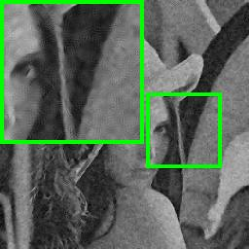
(f) NLM-SAP [44]

(g) NLMNT [27]

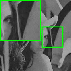
(h) BM3D [29]

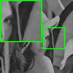
(i) Propose Method

Figure 8: Denoised image obtained using different algorithms for Lena image corrupted with AWGN of $\sigma=40$. The quantitative measures for respective denoised images are (a) PSNR = 27.899, SSIM = 0.745, EKI = 0.7923, (b) PSNR = 28.655, SSIM = 0.832, EKI = 0.889 (c) PSNR = 28.827, SSIM = 0.853, EKI = 898 (d) PSNR = 29.463, SSIM = 0.837, EKI = 0.900 (e) PSNR = 29.233, SSIM = 0.832, EKI = 0.891 (f) PSNR = 29.225, SSIM = 0.842, EKI = 0.886 (g) PSNR = 29.078, SSIM = 0.807, EKI = 881 (h) PSNR = 29.632, SSIM = 0.854, EKI = 0.846 and (i) PSNR = 30.001, SSIM = 0.862, EKI = 0.9101. A patch of each image is magnified for visual assessment.

IV-B Denoising Performance Evaluation

The efficacy of proposed algorithm is investigated for both artificial and natural images corrupted with additive white Gaussian noise (AWGN). Initially,the efficacy of proposed method – in terms of statistical, structural and edge keeping index – is compared with several state-of-the-art denoising techniques for Lena image corrupted with simulated additive noise of $\sigma=40$. Fig.8 illustrates the respective quantitative measures for the following methods: BF [16], Curvelet Thresholding (CT) [11], K-SVD [43], DWT-NeighSURE [6], MBF [22], NLM-SAP [44], NLMNT [27], BM3D [29]. A small patch of each denoised image is magnified (up to $300\%$) to indicate the performance of proposed technique in suppressing noise, while producing sharp edges with minimum loss of fine details even at higher noise strength ($\sigma=40$).

The performance of our method was also investigated on a standard database with images that represent a wide variety of natural scenes. Here, the TID2008 database [15] – that consists of $24$ natural images of different textural characteristic, homogeneous regions and edges – is considered to evaluate the performance of several image denoising algorithms. Initially, all the reference images are converted to grayscale and then resized to $512\times 512$ for uniformity in comparison. Table.III yields the mean PSNR, SSIM and EKI measures for the reference images contaminated with AWGN of $\sigma=[10,20,30,40,50,60,70,75]$. The following few facts may be observed from the comparative analysis:

TABLE III: Mean PSNR (dB), SSIM and EKI Measure between original and restored images for different denoising techniques on TID$2008$ Database [15].

Noise Level	$\sigma=10$	$\sigma=20$	$\sigma=30$	$\sigma=40$	$\sigma=50$	$\sigma=60$	$\sigma=70$	$\sigma=75$
Peak Signal to Noise Ratio (PSNR) in dB
BF [16]	32.333	28.618	26.708	25.479	24.577	23.852	23.238	22.961
CT [11]	31.028	28.045	26.555	25.557	24.823	24.238	23.754	23.544
KSVD [43]	34.593	30.892	28.844	27.405	26.305	25.434	24.719	24.409
NeighSURE [6]	33.535	29.740	27.759	26.474	25.544	24.828	24.255	24.001
MBF [22]	32.669	29.413	27.414	26.245	25.403	24.751	24.212	23.972
NLM-SAP [44]	33.750	30.190	28.145	26.688	25.592	24.744	24.064	23.768
NLMNT [27]	32.821	29.822	27.896	26.379	25.106	24.015	23.058	22.621
BM3D [29]	34.537	30.884	28.863	27.192	26.376	25.530	24.810	24.488
Proposed	33.456	30.186	28.499	27.049	26.179	25.701	25.073	24.526
Structural Similarity Measure [38]
BF [16]	0.9264	0.8550	0.7859	0.7274	0.6768	0.6319	0.5914	0.5725
CT [11]	0.9323	0.8568	0.7965	0.7494	0.7121	0.6811	0.6550	0.6436
KSVD [43]	0.9608	0.9053	0.8519	0.8032	0.7589	0.7188	0.6827	0.6659
NeighSURE [6]	0.9544	0.8947	0.8402	0.7931	0.7521	0.7161	0.6859	0.6713
MBF [22]	0.9314	0.8673	0.8160	0.7722	0.7332	0.6975	0.6642	0.6483
NLM-SAP [44]	0.9504	0.8806	0.8196	0.7666	0.7200	0.6788	0.6420	0.6250
NLMNT [27]	0.9532	0.8955	0.8336	0.7740	0.7187	0.6688	0.6240	0.6035
BM3D [29]	0.9605	0.9096	0.8527	0.8157	0.7762	0.7404	0.7072	0.6914
Proposed	0.9547	0.9122	0.8712	0.8201	0.7893	0.7614	0.7238	0.7014
Edge Keeping Index [42]
BF [16]	0.9395	0.8954	0.8644	0.8416	0.8237	0.8086	0.7952	0.7889
CT [11]	0.9136	0.8776	0.8570	0.8395	0.8240	0.8096	0.7959	0.7894
KSVD [43]	0.9649	0.9346	0.9082	0.8834	0.8598	0.8377	0.8170	0.8073
NeighSURE [6]	0.9534	0.9141	0.8848	0.8624	0.8442	0.8295	0.8174	0.8116
MBF [22]	0.9474	0.9077	0.8770	0.8521	0.8312	0.8129	0.7991	0.7912
NLM-SAP [44]	0.9473	0.9164	0.8906	0.8637	0.8364	0.8101	0.7854	0.7737
NLMNT [27]	0.9305	0.8907	0.8682	0.8444	0.8160	0.7866	0.7601	0.7491
BM3D [29]	0.9620	0.9272	0.8913	0.8386	0.8346	0.8012	0.7672	0.7501
Proposed	0.9514	0.9216	0.8903	0.8790	0.8654	0.8524	0.8328	0.8207

1. The estimation of signal below threshold using JBF aides in attenuating the sudden jumps in Curvelet magnitude and also preservers the essential phase information. The multiscale JBF in coarser scales and BF in the finest scale improves the performance of proposed technique compared to the individual methods of BF [16] and Curvelet Threholding (CT) [11].

2. The approach of GIF as a post-processing ‘Edge-Aware’ filter for the suppression of ringing artifacts and preservation of small image details aides in the enhancement of image quality. The improvement in EKI measures especially at higher noise levels indicate the importance of phase preservation using JBF and the localization of ringing artifacts due to GIF.

3. The multiscale hybrid image denoising technique excelled in performance at higher noise strengths compared to several state-of-the-art image denoising techniques [43, 29, 22]. However its performance is comparable at lower noise levels.

The intra-scale dependencies among the coefficients and the sparse recovery of any curve singularity during reconstruction motivated the authors to use Curvelet transform for image restoration. The multiscale (Joint Bilateral) filtering in Curvelet domain exploits the high co-dependency among the coefficients, while estimating signal residuals from noise subspace. The phases of the estimated magnitudes retain the essential location information of the image features. In contrast to multiscale filtering, spatial domain implementations fail to retain few image details in the low-contrast regions. It is also observed that the BF suffers from gradient reversal artifact near edges [37]. Similarly, the NLM filters search for similar patches in a larger neighboring window, which is again local compared to the whole image [45] and the similarity among patches further decreases with higher noise strength. Thus the performance of NLM-SAP [44] and NLMNT [27] degrades significantly at higher values of $\sigma$. On the other hand, one may notice from Fig.8 that the decimated wavelet transform – in DWT-NeighSURE [6] and MBF [22] – yields distortions of the boundaries and suffers substantial loss of important image detail. A similar observation may also be noticed for Curvelet thresholding [11]. In addition, by setting higher threshold in Curvelet domain to avoid few of these distortion in the finest scale would cause even more of the inherent structure to be missed. We retained these structures using BF. The GIF, as illustrated in Fig.6 localizes the distortions of the boundaries, while keeping the edges, textures and small details of the latent image. Though the block-matching 3D (BM3D) collaborative filter improves the denoising quality significantly, it introduces few visible artifacts in the homogenous regions as shown in Fig.8h. Further, in the absence of similar patches the performance of BM3D deteriorates at higher noise strengths. However, the competitiveness of proposed algorithm is comparable with several state-of-the-art techniques with maximum preservation of image details even at higher noise strength.

V Conclusion

In this article, we proposed a multiscale filtering that improves the performance of classical Curvelet thresholding method for image denoising. The signal estimation in noise subspace using JBF and retention of phase seems to offer advantages in coarser scales, particularly in avoiding visible artifacts. The improvement in EKI measure justifies the importance of phase preservation during image restoration. Our experiments also reveal that Curvelet thresholding in the finest scale suffers substantial loss of important image detail. Therefore, removal of coefficients with thresholds introduces granular artifacts in the denoised image. The proposed BF ensures the elimination of granular artifacts with well-connected edges in the restored image. The reconstructed image is further processed by GIF to reduce the ringing artifacts, which is mostly ignored by many transform domain techniques. We empirically investigated the performance of proposed method under various noise strength to obtain optimum parameter values for JBF and BF in coarser and the finest scales, respectively. The competitiveness of proposed method is examined on TID2008 image database to emphasize its efficacy in diverse fields of applications. The experimental results illustrated the consistency of proposed algorithm compared to several state-of-the-art image denoising techniques.

References

- [1] D. L. Donoho and J. M. Johnstone, “Ideal spatial adaptation by wavelet shrinkage,” Biometrika, vol. 81, no. 3, pp. 425–455, 1994.
- [2] D. L. Donoho, I. M. Johnstone, G. Kerkyacharian, and D. Picard, “Wavelet shrinkage: asymptopia?” Journal of the Royal Statistical Society. Series B (Methodological), pp. 301–369, 1995.
- [3] S. G. Chang, B. Yu, and M. Vetterli, “Adaptive wavelet thresholding for image denoising and compression,” Image Processing, IEEE Transactions on, vol. 9, no. 9, pp. 1532–1546, 2000.
- [4] L. Sendur and I. W. Selesnick, “Bivariate shrinkage functions for wavelet-based denoising exploiting interscale dependency,” IEEE Transactions on signal processing, vol. 50, no. 11, pp. 2744–2756, 2002.
- [5] A. Pizurica and W. Philips, “Estimating the probability of the presence of a signal of interest in multiresolution single-and multiband image denoising,” IEEE Transactions on image processing, vol. 15, no. 3, pp. 654–665, 2006.
- [6] Z. Dengwen and C. Wengang, “Image denoising with an optimal threshold and neighbouring window,” Pattern Recognition Letters, vol. 29, no. 11, pp. 1694–1697, 2008.
- [7] F. Luisier, T. Blu, and M. Unser, “Sure-let for orthonormal wavelet-domain video denoising,” IEEE Transactions on Circuits and Systems for Video Technology, vol. 20, no. 6, pp. 913–919, 2010.
- [8] J. Portilla, V. Strela, M. J. Wainwright, and E. P. Simoncelli, “Image denoising using scale mixtures of gaussians in the wavelet domain,” Image Processing, IEEE Transactions on, vol. 12, no. 11, pp. 1338–1351, 2003.
- [9] D. Lazzaro and L. Montefusco, “Edge-preserving wavelet thresholding for image denoising,” Journal of Computational and Applied Mathematics, vol. 210, no. 1, pp. 222–231, 2007.
- [10] B. Tekin, U. S. Kamilov, E. Bostan, and M. Unser, “Benefits of consistency in image denoising with steerable wavelets,” in 2013 IEEE International Conference on Acoustics, Speech and Signal Processing. Ieee, 2013, pp. 1355–1358.
- [11] J.-L. Starck, E. J. Candès, and D. L. Donoho, “The curvelet transform for image denoising,” Image Processing, IEEE Transactions on, vol. 11, no. 6, pp. 670–684, 2002.
- [12] J. Ma and G. Plonka, “Combined curvelet shrinkage and nonlinear anisotropic diffusion,” IEEE Transactions on Image processing, vol. 16, no. 9, pp. 2198–2206, 2007.
- [13] ——, “The curvelet transform,” Signal Processing Magazine, IEEE, vol. 27, no. 2, pp. 118–133, 2010.
- [14] N. Remenyi, O. Nicolis, G. Nason, and B. Vidakovic, “Image denoising with 2d scale-mixing complex wavelet transforms,” Image Processing, IEEE Transactions on, vol. 23, no. 12, pp. 5165–5174, 2014.
- [15] N. Ponomarenko, V. Lukin, A. Zelensky, K. Egiazarian, M. Carli, and F. Battisti, “Tid2008-a database for evaluation of full-reference visual quality assessment metrics,” Advances of Modern Radioelectronics, vol. 10, no. 4, pp. 30–45, 2009.
- [16] C. Tomasi and R. Manduchi, “Bilateral filtering for gray and color images,” in Computer Vision, 1998. Sixth International Conference on. IEEE, 1998, pp. 839–846.
- [17] A. Buades, B. Coll, and J.-M. Morel, “A review of image denoising algorithms, with a new one,” Multiscale Modeling & Simulation, vol. 4, no. 2, pp. 490–530, 2005.
- [18] H. Takeda, S. Farsiu, and P. Milanfar, “Kernel regression for image processing and reconstruction,” Image Processing, IEEE Transactions on, vol. 16, no. 2, pp. 349–366, 2007.
- [19] L. Yaroslavsky, Digital picture processing: an introduction. Springer Science & Business Media, 2012, vol. 9.
- [20] P. Milanfar, “A tour of modern image filtering: New insights and methods, both practical and theoretical,” IEEE Signal Processing Magazine, vol. 30, no. 1, pp. 106–128, 2013.
- [21] G. Petschnigg, R. Szeliski, M. Agrawala, M. Cohen, H. Hoppe, and K. Toyama, “Digital photography with flash and no-flash image pairs,” ACM transactions on graphics (TOG), vol. 23, no. 3, pp. 664–672, 2004.
- [22] M. Zhang and B. K. Gunturk, “Multiresolution bilateral filtering for image denoising,” Image Processing, IEEE Transactions on, vol. 17, no. 12, pp. 2324–2333, 2008.
- [23] B. K. Shreyamsha Kumar, “Image denoising based on gaussian/bilateral filter and its method noise thresholding,” Signal, Image and Video Processing, vol. 7, no. 6, pp. 1159–1172, 2013. [Online]. Available: http://dx.doi.org/10.1007/s11760-012-0372-7
- [24] K. Wu, X. Zhang, and M. Ding, “Curvelet based nonlocal means algorithm for image denoising,” AEU-International Journal of Electronics and Communications, vol. 68, no. 1, pp. 37–43, 2014.
- [25] X. Zhang, “Image denoising using local wiener filter and its method noise,” Optik-International Journal for Light and Electron Optics, vol. 127, no. 17, pp. 6821–6828, 2016.
- [26] C. Knaus and M. Zwicker, “Dual-domain image denoising,” in Image Processing (ICIP), 2013 20th IEEE International Conference on. IEEE, 2013, pp. 440–444.
- [27] B. S. Kumar, “Image denoising based on non-local means filter and its method noise thresholding,” Signal, image and video processing, vol. 7, no. 6, pp. 1211–1227, 2013.
- [28] G. Easley, D. Labate, and W.-Q. Lim, “Sparse directional image representations using the discrete shearlet transform,” Applied and Computational Harmonic Analysis, vol. 25, no. 1, pp. 25–46, 2008.
- [29] K. Dabov, A. Foi, V. Katkovnik, and K. Egiazarian, “Image denoising by sparse 3-d transform-domain collaborative filtering,” IEEE Transactions on image processing, vol. 16, no. 8, pp. 2080–2095, 2007.
- [30] C. Knaus and M. Zwicker, “Progressive image denoising,” IEEE transactions on image processing, vol. 23, no. 7, pp. 3114–3125, 2014.
- [31] S. Ghosh and K. N. Chaudhury, “On fast bilateral filtering using fourier kernels,” IEEE Signal Processing Letters, vol. 23, no. 5, pp. 570–573, 2016.
- [32] N. Skarbnik, Y. Y. Zeevi, and C. Sagiv, “The importance of phase in image processing,” Ph.D. dissertation, Technion-Israel Institute of Technology, Faculty of Electrical Engineering, 2009.
- [33] S. K. Panigrahi and S. Gupta, “Quantitative evaluation of image information retention by relative phases,” in Engineering and Systems (SCES), 2013 Students Conference on. IEEE, 2013, pp. 1–6.
- [34] S. K. Panigrahi, S. Gupta, and P. K. Sahu, “Phases under gaussian additive noise,” in Communication and Signal Processing (ICCSP), 2016 International Conference on. IEEE, 2016, pp. 1771–1776.
- [35] L. Boubchir and J. Fadili, “Multivariate statistical modeling of images with the curvelet transform.” in ISSPA, 2005, pp. 747–750.
- [36] H. Rabbani, M. Vafadust, and S. Gazor, “Image denoising in curvelet transform domain using gaussian mixture model with local parameters for distribution of noise-free coefficients,” in Medical Devices and Biosensors, 2007. ISSS-MDBS 2007. 4th IEEE/EMBS International Summer School and Symposium on. IEEE, 2007, pp. 57–60.
- [37] K. He, J. Sun, and X. Tang, “Guided image filtering,” IEEE transactions on pattern analysis and machine intelligence, vol. 35, no. 6, pp. 1397–1409, 2013.
- [38] Z. Wang, A. C. Bovik, H. R. Sheikh, and E. P. Simoncelli, “Image quality assessment: from error visibility to structural similarity,” Image Processing, IEEE Transactions on, vol. 13, no. 4, pp. 600–612, 2004.
- [39] E. Luo, S. H. Chan, and T. Q. Nguyen, “Adaptive image denoising by targeted databases,” IEEE Transactions on Image Processing, vol. 24, no. 7, pp. 2167–2181, 2015.
- [40] A. Hore and D. Ziou, “Image quality metrics: Psnr vs. ssim,” in Pattern recognition (icpr), 2010 20th international conference on. IEEE, 2010, pp. 2366–2369.
- [41] K. Zeng and Z. Wang, “Perceptual evaluation of image denoising algorithms,” in 2013 Asilomar Conference on Signals, Systems and Computers. IEEE, 2013, pp. 1351–1355.
- [42] H. Bhadauria and M. Dewal, “Medical image denoising using adaptive fusion of curvelet transform and total variation,” Computers & Electrical Engineering, vol. 39, no. 5, pp. 1451–1460, 2013.
- [43] M. Elad and M. Aharon, “Image denoising via sparse and redundant representations over learned dictionaries,” IEEE Transactions on Image processing, vol. 15, no. 12, pp. 3736–3745, 2006.
- [44] C.-A. Deledalle, V. Duval, and J. Salmon, “Non-local methods with shape-adaptive patches (nlm-sap),” Journal of Mathematical Imaging and Vision, vol. 43, no. 2, pp. 103–120, 2012.
- [45] A. Buades, B. Coll, and J.-M. Morel, “Non-local means denoising,” Image Processing On Line, vol. 1, pp. 208–212, 2011.