Near-field imaging of an unbounded elastic rough surface with a direct imaging method

Abstract

This paper is concerned with the inverse scattering problem of time-harmonic elastic waves by an unbounded rigid rough surface. A direct imaging method is developed to reconstruct the unbounded rough surface from the elastic scattered near-field Cauchy data generated by point sources. A Helmholtz-Kirchhoff-type identity is derived and then used to provide a theoretical analysis of the direct imaging algorithm. Numerical experiments are presented to show that the direct imaging algorithm is fast, accurate and robust with respect to noise in the data.

1 Introduction

Elastic scattering problems have received much attention from both the engineering and mathematical communities due to their significant applications in diverse scientific areas such as seismology, remote sensing, geophysics and nondestructive testing.

This paper focuses on the inverse problem of scattering of time-harmonic elastic waves by an unbounded rough surface. The domain above the rough surface is filled with a homogeneous and isotropic elastic medium, and the medium below the surface is assumed to be elastically rigid. Our purpose is to image the unbounded rough surface from the scattered elastic near-field Cauchy data measured on a horizontal straight line segment above the rough surface and generated by point sources. For simplicity, in this paper, we are restricted to the two-dimensional case. See Fig. 1 for the problem geometry. However, our imaging algorithm can be generalized to the three-dimensional case with appropriate modifications.

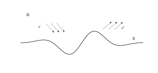
Fig. 1: The elastic scattering problem by a Dirichlet rough surface.

For inverse acoustic scattering problems by unbounded rough surfaces, many numerical reconstruction methods have been developed to recover the unbounded surfaces, such as the sampling method in [7, 37, 38, 39] for reconstructing periodic structures, the time-domain probe method in [11], the time-domain point source method in [17] and the nonlinear integral equation method in [26] for recovering sound-soft rough surfaces, the transformed field expansion method in [9, 10] for reconstructing a small and smooth deformation of a flat surface with Dirichlet, impedance or transmission conditions, the Kirsch-Kress method in [27] for a penetrable locally rough surface, the Newton iterative method in [41] for a sound-soft locally rough surface, and the direct imaging method in [33] for imaging impenetrable or penetrable unbounded rough surfaces from the scattered near-field Cauchy data.

Compared with the acoustic case, elastic scattering problems are more complicated due to the coexistence of the compressional and shear waves that propagate at different speeds. This makes the elastic scattering problems more difficult to deal with theoretically and numerically. For inverse scattering by bounded elastic bodies, several numerical inversion algorithms have been proposed, such as the sampling method in [6, 8, 16, 35, 40] and the transformed field expansion method in [28, 29, 30]. See also the monograph [2] for a good survey. However, as far as we know, not many results are available for inverse elastic scattering by unbounded rough surfaces. An optimization method was proposed in [20] to reconstruct an elastically rigid periodic surface, a factorization method was developed in [21] for imaging an elastically rigid periodic surface and in [22] for reconstructing bi-periodic interfaces between acoustic and elastic media, and the transformed field expansion method was given in [31] for imaging an elastically rigid bi-periodic surface.

The purpose of this paper is to develop a direct imaging method for inverse elastic scattering problems by an unbounded rigid rough surface (on which the elastic displacement vanishes). The main idea of a direct imaging method is to present a certain imaging function to determine whether or not a sampling point in the sampling area is on the obstacle. Direct imaging methods usually require very little priori information of the obstacle, and the imaging function usually involves only the measurement data but not the solution of the scattering problem and thus can be computed easily and fast. This is especially important for the elastic case since the computation of the elastic scattering solution is very time-consuming. Due to the above features, direct imaging methods have recently been studied by many authors for inverse scattering by bounded obstacles or inhomogeneity, such as the orthogonality sampling method [36], the direct sampling method [23, 24, 25, 34], the reverse time migration method [13, 14] and the references quoted there. Recently, a direct imaging method was proposed in [33] to reconstruct unbounded rough surfaces from the acoustic scattered near-field Cauchy data generated by acoustic point sources. This paper is a nontrivial extension of our recent work in [33] from the acoustic case to the elastic case since the elastic case is much more complicated than the acoustic case due to the coexistence of the compressional and shear waves that propagate at different speeds.

To understand why our direct imaging method works, a theoretical analysis is presented, based on an integral identity concerning the fundamental solution of the Navier equation (see Lemma 7) which is established in this paper. This integral identity is similar to the Helmholtz-Kirchhoff identity for bounded obstacles in [14]. In addition, a reciprocity relation (see Lemma 8) is proved for the elastic scattered field corresponding to the unbounded rough surface. Based on these results, the required imaging function is then proposed, which, at each sampling point, involves only the inner products of the measured data and the fundamental solution of the Navier equation in a homogeneous background medium. Thus, the computation cost of the imaging function is very cheap. Numerical results are consistent with the theoretical analysis and show that our imaging method can provide an accurate and reliable reconstruction of the unbounded rough surface even in the presence of a fairly large amount of noise in the measured data.

The remaining part of the paper is organized as follows. In Section 2, we formulate the elastic scattering problem and present some inequalities that will be used in this paper. Moreover, the well-posedness of the forward scattering problem is presented, based on the integral equation method (see [3, 4, 5]). Section 3 provides a theoretical analysis of the continuous imaging function. Based on this, a novel direct imaging method is proposed for the inverse elastic scattering problem. Numerical examples are carried out in Section 4 to illustrate the effectiveness of the imaging method. In the appendix, we present two lemmas which are needed for the proof of the reciprocity relation.

We conclude this section by introducing some notations used throughout the paper. For any open set $D\subset{\mathbb{R}}^{m}\,\,(m\in{\mathbb{N}})$, denote by $BC(D)$ the set of bounded and continuous, complex-valued functions in $D$, a Banach space under the norm $\|\varphi\|_{\infty,D}:=\sup_{x\in D}|\varphi(x)|$. Given a function $v\in L^{\infty}(D)$, denote by $\partial_{j}v$ the (distributional) derivative $\partial v(x)/\partial x_{j}$, $j=1,\cdots,m$. Define $BC^{1,1}(D):=\{\varphi\in BC(D)~{}|~{}\partial_{j}\varphi\in BC(D),j=1,\cdots,m\}$, equipped with the norm $\|\varphi\|_{1,D}:=\|\varphi\|_{\infty,D}+\sum_{j=1}^{m}\|\partial_{j}\varphi\|_{\infty,D}$. The space of Hölder continuous functions is denoted by $C^{0,\alpha}(\overline{D}):=\{\varphi\in C(\overline{D}):\|\varphi\|_{0,\alpha;D}\}$ with the norm $\|\varphi\|_{0,\alpha,D}:=\|\varphi\|_{\infty;D}+\sup_{x,y\in D,x\neq y}[|\varphi(x)-\varphi(y)|/|x-y|^{\alpha}]$. Denote by $C^{1,\alpha}({\mathbb{R}})$ the space of uniformly Hölder continuously differentiable functions or the space of differentiable functions $\varphi$ for which $\nabla\varphi$ belongs to $C^{0,\alpha}({\mathbb{R}})$ with the norm $\|\varphi\|_{1,\alpha}:=\|\varphi\|_{\infty;D}+\|\nabla\varphi\|_{0,\alpha}$. We will also make use of the standard Sobolev space $H^{1}(D)$ for any open set $D\subset{\mathbb{R}}^{2}$ and $H^{1/2}(\partial D)$ provided the boundary of $D$ is smooth enough. The notations $H^{1}_{loc}(\partial D)$ and $H^{1/2}_{loc}(D)$ denote the functions which are the elements of $H^{1/2}(\partial E)$ and $H^{1}(E)$ for any $E\subset\subset D$, respectively.

2 Problem formulation

In this section, we formulate the elastic scattering problem considered in this paper and present its well-posedness results. Useful notations and inequalities used in the paper will also be given.

2.1 The forward elastic scattering problem

The propagation of time-harmonic waves with circular frequency $\omega$ in an elastic solid with Lamé constants $\mu,\lambda~{}(\mu>0,\lambda+\mu\geq 0)$ is governed by the Navier equation

$$\Delta^{*}{\bm{u}}+\omega^{2}{\bm{u}}=0.$$ (2.1)

Here, ${\bm{u}}=(u_{1},u_{2})^{T}$ denotes the displacement field and

$$\Delta^{*}{\bm{u}}:=\mu\Delta{\bm{u}}+(\lambda+\mu)\text{grad div}\,{\bm{u}}.$$

We consider a two-dimensional unbounded rough surface $S:=\{x=(x_{1},x_{2})\in{\mathbb{R}}^{2}\;|\;x_{2}=f(x_{1})\}$, where $S$ is the surface profile function satisfying that $f\in BC^{1,1}({\mathbb{R}})$. Denote by $\Omega$ the region above $S$. Throughout the paper, the letters $h$ and $H$ will be frequently used to denote certain real numbers satisfying that $h<\inf f=:f_{-}$ and $H>\sup f=:f_{+}$. For any $a\in{\mathbb{R}}$, introduce the sets

$$U_{a}:=\{{x}=(x_{1},x_{2})\in\mathbb{R}^{2}:x_{2}>a\},\qquad T_{a}:=\{{x}=(x_{1},x_{2})\in\mathbb{R}^{2}:x_{2}=a\}.$$

Let $\Gamma({x,y})$ be the free-space Green’s tensor for the two-dimensional Navier equation:

$$\Gamma({x,y}):=\frac{1}{\mu}{\bm{I}}\varPhi_{k_{s}}({x,y})+\frac{1}{\omega^{2}}\nabla^{T}_{x}\nabla_{x}\left(\varPhi_{k_{s}}({x,y})-\varPhi_{k_{p}}({x,y})\right),$$ (2.2)

with ${x,y}\in\mathbb{R}^{2},~{}{x\neq y}$, where the scalar function $\varPhi_{k}({x,y})$ is the fundamental solution to the two-dimensional Helmholtz equation given by

$$\varPhi_{k}({x,y}):=\frac{i}{4}H^{(1)}_{0}(k|{x-y}|),\quad{x\not=y},$$ (2.3)

and the compressional wave number $k_{p}$ and the shear wave number $k_{s}$ are given by

$$k_{p}:={\omega}/{\sqrt{2\mu+\lambda}},\quad k_{s}:={\omega}/{\sqrt{\mu}}.$$

Motivated by the form of the corresponding Green’s function for acoustic wave propagation, we define the Green’s tensor $\Gamma_{D,h}({x,y})$ for the first boundary value problem of elasticity in the half-space $U_{h}$ by

$$\Gamma_{D.h}({x,y}):=\Gamma({x,y})-\Gamma({x,y^{\prime}_{h}})+U({x,y}),\quad{x,y}\in U_{h},\;{x\neq y}.$$

Here, $y^{\prime}_{h}=(y_{1},2h-y_{2})$ and the matrix function $U$ is analytic. For more properties of $U$ we refer to [3, Chapter 2.4].

Given a curve $\Lambda\subset\mathbb{R}^{2}$ with the unit normal vector ${\bm{n}}=(n_{1},n_{2})$, the generalised stress vector ${\bm{P}}$ on $\Lambda$ is defined by

$${\bm{P}\bm{u}}:=(\mu+\tilde{\mu})\frac{\partial{\bm{u}}}{\partial\bm{n}}+\tilde{\lambda}{\bm{n}}~{}\text{div}~{}{\bm{u}}-\tilde{\mu}~{}{\bm{n}}^{\perp}\text{div}^{\perp}{\bm{u}},\quad\text{div}^{\perp}:=(-\partial_{2},\partial_{1}).$$ (2.4)

Here, $\tilde{\mu},\tilde{\lambda}$ are real numbers satisfying $\tilde{\mu}+\tilde{\lambda}=\mu+\lambda$ and ${\bm{n}}^{\perp}:=(-n_{2},n_{1})$.

If we apply the generalised stress operator ${\bm{P}}$ to $\Gamma$ and $\Gamma_{D,h}$, we obtain the matrix functions $\Pi^{(1)},\Pi^{(2)},\Pi^{(1)}_{D,h}$ and $\Pi^{(2)}_{D,h}$:

$$\Pi^{(1)}_{jk}({x,y}) :=\left({\bm{P}}^{({x})}\left(\Gamma_{\cdot k}({x,y})\right)\right)_{j},$$ (2.5)

$$\Pi^{(2)}_{jk}({x,y}) :=\left({\bm{P}}^{({y})}\left(\Gamma_{j\cdot}({x,y})\right)^{T}\right)_{k},$$ (2.6)

$$\Pi^{(1)}_{D,h,jk}({x,y}) :=\left({\bm{P}}^{({x})}\left(\Gamma_{D,h,\cdot k}({x,y})\right)\right)_{j},$$ (2.7)

$$\Pi^{(2)}_{D,h,jk}({x,y}) :=\left({\bm{P}}^{({y})}\left(\Gamma_{D,h,\cdot j}({x,y})\right)^{T}\right)_{k}.$$ (2.8)

Given the incident wave $\bm{u}^{i}$, the scattered field ${\bm{u}^{s}}=\bm{u}-\bm{u}^{i}$ is required to fulfill the upwards propagating radiation condition (UPRC) (see [4]):

$${\bm{u}}^{s}(x)=\int_{T_{H}}\Pi^{(2)}_{D.H}({x,y})\bm{\phi}({y})ds({y}),\quad{x}\in U_{H}$$ (2.9)

with some $\bm{\phi}\in[L^{\infty}(\Gamma_{H})]^{2}$.

We reformulate the elastic scattering problem by the unbounded rough surface $S$ as the following boundary value problem:

Problem 1.

Given a vector field ${\bm{g}}\in[BC(S)\cap H^{1/2}_{loc}(S)]^{2}$, find a vector field $\bm{u}^{s}\in[C^{2}(\Omega)\cap C(\overline{\Omega})\cap H^{1}_{loc}(\Omega)]^{2}$ that satisfies

1) the Navier equation (2.1) in $\Omega$,

2) the Dirichlet boundary condition $\bm{u}^{s}=\bm{g}$ on $S$,

3) the vertical growth rate condition: $\sup_{{x}\in\Omega}|x_{2}|^{\beta}|{\bm{u}}^{s}(x)|<\infty$ for some $\beta\in\mathbb{R}$,

4) the UPRC (2.9).

Remark 2.

In Problem 1, the boundary data is determined by the incident wave ${\bm{u}}^{i}$, that is, ${\bm{g}:=-{\bm{u}}}^{i}|_{S}$.

2.2 Some useful notations

We give some basic notations and fundamental functions that will be needed in the subsequent discussions.

The fundamental solution $\Gamma$ defined in (2.2) can be decomposed into the compressional and shear components [1]:

$$\Gamma(x,y)=\Gamma_{p}(x,y)+\Gamma_{s}(x,y),\quad x,y\in{\mathbb{R}}^{2},\quad x\not=0,$$

where

$$\Gamma_{p}(x,y)=-\frac{1}{\mu k_{s}^{2}}\nabla^{T}_{x}\nabla^{T}_{x}\varPhi_{k_{p}}(x,y)\quad\text{and}\quad\Gamma_{s}(x,y)=\frac{1}{\mu k_{s}^{2}}(k_{s}^{2}\bm{I}+\nabla^{T}_{x}\nabla^{T}_{x})\varPhi_{k_{s}}(x,y).$$

The asymptotic behavior of these functions have been given in [2, Proposition 1.14]:

$$\Gamma_{p}(x,y)=\frac{k_{p}^{2}}{\omega}\varPhi_{k_{p}}(x,y)\widehat{{y-x}}\otimes\widehat{{y-x}}+o\left({|x-y|}^{-1}\right),$$ (2.10)

$$\Gamma_{s}(x,y)=\frac{k_{s}^{2}}{\omega}\varPhi_{k_{s}}(x,y)\left(\bm{I}-\widehat{{y-x}}\otimes\widehat{{y-x}}\right)+o\left({|x-y|}^{-1}\right),$$ (2.11)

$$\Pi^{(1)}_{\alpha}(x,y)\bm{q}=i\omega^{2}/k_{\alpha}\Gamma_{\alpha}(x,y)\bm{q}+o\left({|x-y|}^{-1}\right),$$ (2.12)

where $\alpha=s,p$, $\Pi^{(1)}_{\alpha}$ is defined in (2.5) with $\bm{n}(x)={(x-y)}/{|x-y|}$ and for any vector $\bm{v}=(v_{1},v_{2})^{T},$

$$\bm{v}\otimes\bm{v}=\bm{v}\bm{v}^{T}=\left[\begin{matrix}v_{1}^{2}&v_{1}v_{2}\\ v_{2}v_{1}&v_{2}^{2}\end{matrix}\right].$$ (2.13)

From [3, (2.14) and (2.29)] there exists a constant $C>0$ such that for ${x,y}\in U_{h},$

$$\max\limits_{j,k=1,2}|\Gamma_{jk}({x,y})|\leq C(1+|\log|{x-y}|),$$ (2.14)

$$\max\limits_{j,k=1,2}|\Gamma_{D,h,jk}({x,y})|\leq C(1+|\log|{x-y}|).$$ (2.15)

Further, we have the following asymptotic property of the Hankel functions and their derivatives [15]: For fixed $n\in\mathbb{N}$,

$$H^{(1)}_{n}(t) = \sqrt{\frac{2}{\pi t}}e^{i(t-\frac{n\pi}{2}-\frac{\pi}{4})}\left\{1+O\left(\frac{1}{t}\right)\right\},\quad t\to\infty,$$ (2.16)

$$H^{(1)^{\prime}}_{n}(t) = \sqrt{\frac{2}{\pi t}}e^{i(t-\frac{n\pi}{2}+\frac{\pi}{4})}\left\{1+O\left(\frac{1}{t}\right)\right\},\quad t\to\infty.$$ (2.17)

By (2.16) and (2.17), we can deduce that

$$\Gamma({x,y})\leq C(k_{s},k_{p},\delta)\left[\begin{matrix}|{x-y}|^{-\frac{1}{2}}&|{x-y}|^{-\frac{3}{2}}\\ |{x-y}|^{-\frac{3}{2}}&|{x-y}|^{-\frac{1}{2}}\end{matrix}\right]\quad\text{as}\quad|x_{1}|\rightarrow\infty$$ (2.18)

for ${x,y}\in U_{h}$ with $|x_{1}-y_{1}|>\delta$, where $\delta>0$ is a constant. Combining this with (2.4)-(2.6) gives

$$\Pi^{(1)}({x,y})\leq C(k_{s},k_{p},\delta)\left[\begin{matrix}|{x-y}|^{-\frac{3}{2}}&|{x-y}|^{-\frac{1}{2}}\\ |{x-y}|^{-\frac{1}{2}}&|{x-y}|^{-\frac{3}{2}}\end{matrix}\right]\quad\text{as}\quad|x_{1}|\rightarrow\infty.$$ (2.19)

Further, we also need the following inequalities (see [3, Theorems 2.13 and 2.16 (a)]:

$$\max\limits_{j,k=1,2}|\Gamma_{D,h,jk}(x,y)|\leq\frac{\mathscr{H}(x_{2}-h,y_{2}-h)}{|x_{1}-y_{1}|^{3/2}},$$ (2.20)

$$\max\limits_{j,k=1,2}|\Pi^{(1)}_{D,h,jk}(x,y)|\leq\frac{\mathscr{H}(x_{2}-h,y_{2}-h)}{|x_{1}-y_{1}|^{3/2}},$$ (2.21)

$$\max\limits_{j,k=1,2}|\Pi^{(2)}_{D,h,jk}(x,y)|\leq\frac{\mathscr{H}(x_{2}-h,y_{2}-h)}{|x_{1}-y_{1}|^{3/2}},$$ (2.22)

$$\sup_{x\in T_{H}}\int_{S}\max\limits_{j,k=1,2}|\mathscr{G}_{jk}(x,y)|ds(y)<\infty$$ (2.23)

for $|x_{1}-y_{1}|>\delta>0$, where $\mathscr{G}_{jk}$ denotes any derivative with respect to $x$ of $\Pi^{(2)}_{D,h,jk}$ and $\mathscr{H}\in C({\mathbb{R}}^{2})$. For detailed properties of $\Gamma$, $\Gamma_{D,h}$, $\Pi^{(i)}$ and $\Pi^{(i)}_{D,h},~{}i=1,2$ can be found in [3, Section 2.3-2.4].

2.3 Well-posedness of the forward scattering problem

The well-posedness of the elastic scattering problem reformulated as Problem 1 has been studied in [3, 4, 5] by the integral equation method or in [18, 19] by a variational approach. We present the well-posedness results obtained in [3, 4, 5] by the integral equation method, which will be needed in this paper. To this end, we introduce the elastic layer potentials. For a vector-valued density ${\bm{\varphi}}\in[BC(S)]^{2}$, we define the elastic single-layer potential by

$${\bm{V\varphi}(x)}:=\int_{S}\Gamma_{D,h}(x,y){\bm{\varphi}}(y)ds(y)\quad{x}\in U_{h}\backslash S,$$ (2.24)

and the elastic double-layer potential by

$${\bm{W\varphi}(x)}:=\int_{S}\Pi^{(2)}_{D,h}(x,y){\bm{\varphi}}(y)ds(y)\quad{x}\in U_{h}\backslash S.$$ (2.25)

From the properties of $\Gamma_{D,h}$ and $\Pi^{(2)}_{D,h}$ (see [3, Chapter 2]) it follows that the above integrals exist as improper integrals. Further, it is easy to verify that the potentials $\bm{V\varphi}$ and $\bm{W\varphi}$ are solutions to the Navier equation in both $U_{h}\backslash\overline{\Omega}$ and $\Omega$. We now seek a solution to Problem 1 in the form of a combined single- and double-layer potential

$${\bm{u}}^{s}(x)=\int_{S}\left\{\Pi^{(2)}_{D,h}(x,y)-i\eta\Gamma_{D,h}(x,y)\right\}{\bm{\varphi}}(y)ds(y),\quad{x}\in\Omega,$$ (2.26)

where ${\bm{\varphi}}\in[BC(S)\cap H^{1/2}_{loc}(S)]^{2}$ and $\eta$ is a complex number with ${\rm Re}(\eta)>0$. From [5, pp. 10] we know that $\bm{u}^{s}$ is a solution to the boundary value Problem 1 if $\bm{\varphi}$ is a solution to the integral equation

$$\frac{1}{2}\bm{\varphi}({x})+\int_{S}\left\{\Pi^{(2)}_{D,h}({x,y})-i\eta\Gamma_{D,h}({x,y})\right\}\bm{\varphi}(y)ds(y)=-{\bm{g}(x)},\quad{x}\in S.$$ (2.27)

Introduce the three integral operators ${\bm{S}}_{f}$, ${\bm{D}}_{f}$ and ${\bm{D}^{\prime}}_{f}$:

$${\bm{S}}_{f}\bm{\phi}(s) := 2\int_{-\infty}^{\infty}\Gamma_{D,h}((s,f(s)),(t,f(t)))\bm{\phi}(t)\sqrt{1+f^{\prime}(t)^{2}}dt,$$

$${\bm{D}}_{f}\bm{\phi}(s) := 2\int_{-\infty}^{\infty}\Pi^{(2)}_{D,h}((s,f(s)),(t,f(t)))\bm{\phi}(t)\sqrt{1+f^{\prime}(t)^{2}}dt,$$

$${\bm{D}}^{\prime}_{f}\bm{\phi}(s) := 2\int_{-\infty}^{\infty}\Pi^{(1)}_{D,h}((s,f(s)),(t,f(t)))\bm{\phi}(t)\sqrt{1+f^{\prime}(t)^{2}}dt,$$

where $s\in{\mathbb{R}}$ and $\bm{\phi}\in[L^{\infty}({\mathbb{R}})]^{2}$. From [3, Theorems 3.11 (c) and 3.12 (b)], we know that these three operators are bounded mappings from $[BC({\mathbb{R}})]^{2}$ into $[C^{0,\alpha}({\mathbb{R}})]^{2}$. Set $\bm{\phi}(s)=\bm{\varphi}(s,f(s))$. Then the integral equation (2.27) is equivalent to

$$({\bm{I}}+{\bm{D}}_{f}-i\eta{\bm{S}}_{f})\phi(s)=-2{\bm{g}}(s,f(s)),\quad s\in\mathbb{R}.$$ (2.28)

The unique solvability of (2.28) was shown in [3, 4, 5] in both the space of bounded and continuous functions and $L^{p}({\mathbb{R}})$, $1\leq p\leq\infty$, yielding existence of solutions to Problem 1. We just present the conclusions that will be used in the next sections; see [3, Chapter 5] or [4, 5] for details.

Theorem 3.

([3, Corollary 5.23] or [5, Corollary 5.12]) The operator ${\bm{I}}+{\bm{D}}_{f}-i\eta{\bm{S}}_{f}$ is bijective on $[BC({\mathbb{R}})]^{2}$, and there holds

$$\|({\bm{I}}+{\bm{D}}_{f}-i\eta{\bm{S}}_{f})^{-1}\|<\infty.$$

For the original scattering problem formulated as a boundary value problem, Problem 1, we have the following well-posedness result.

Theorem 4.

([3, Theorem 5.24] or [5, Theorem 5.13]) For any Dirichlet data ${\bm{g}}\in[BC(S)\cap H^{1/2}_{loc}(S)]^{2}$, there exists a unique solution ${\bm{u}}^{s}\in[C^{2}(\Omega)\cap C(\overline{\Omega})\cap H^{1}_{loc}(\Omega)]^{2}$ to Problem 1 which depends continuously on $\|{\bm{g}}\|_{\infty;S}$, uniformly in $[C(\overline{\Omega}\setminus U_{H})]^{2}$ for any $H>\sup f$.

3 The imaging algorithm

For $H>f_{+}$ and $A>0$ let $T_{H,A}:=\{x\in\Omega\,|\,x_{2}=H,|x_{1}|<A\}$ be a horizontal line segment above the rough surface $S$. Then our inverse scattering problem is to determine $S$ from the scattered near-field Cauchy data $\{(\bm{u}^{s}(x;y),\bm{P}\bm{u}^{s}(x;y))\;|\;x,y\in T_{H}\}$ corresponding to the elastic incident point sources $\bm{u}^{i}(x;y,\bm{e}_{j}):=\Gamma(x;y)\bm{e}_{j},j=1,2$. Here, $\bm{e}_{1}=(1\;0)^{T},\bm{e}_{2}=(0\;1)^{T}$.

We will present a novel direct imaging method to recover the unbounded rough surface $S$. To this end, we first establish certain results for the forward scattering problem associated with incident point sources. The imaging function for the inverse problem will then be given at the end of this section. In the following proofs, the constant $C>0$ may be different at different places.

Lemma 5.

Assume that ${\bm{u}}^{s}$ is the solution to Problem 1 with the boundary data ${\bm{g}}=(g_{1},g_{2})^{T}$. If ${\bm{g}}\in[L^{p}({S})]^{2}$ with $1\leq p\leq\infty$, then ${\bm{u}}^{s},{\bm{Pu}^{s}}\in[L^{r}(T_{H})]^{2}$ for any $H-f_{+}\geq\delta>0$ and ${1}/{r}<{1}/{2}+{1}/{p}$.

Proof.

From (2.26), the scattered field ${\bm{u}}^{s}$ can be written in the form

$${\bm{u}}^{s}(x)=\int_{S}\left\{\Pi^{(2)}_{D,h}({x,y})-i\eta\Gamma_{D,h}({x,y})\right\}\bm{\varphi}(y)ds(y),\quad{x}\in\Omega,$$ (3.1)

where $\bm{\varphi}\in[L^{p}({S})]^{2}$ is the unique solution to the boundary integral equation (2.27).

The inequalities (2.20) and (2.22) imply that

$$\max\limits_{j,k=1,2}|\Pi^{(2)}_{D,h,jk}(x,y)-i\eta\Gamma_{D,h,jk}(x,y)|\leq\frac{\mathscr{H}(x_{2}-h,y_{2}-h)}{|x_{1}-y_{1}|^{3/2}}\in L^{{3}/{2}+\varepsilon}({\mathbb{R}}^{2}),\;\;\forall\varepsilon>0.$$

This, combined with (3.1) and Young’s inequality, implies that

$${\bm{u}}^{s}\in[L^{r}(T_{H})]^{2}\quad\text{with}\quad{1}/{r}<{1}/{2}+{1}/{p}.$$

Further, by (3.1) we deduce that for ${x}\in T_{H}$

$${\bm{P}^{(x)}}{\bm{u}}^{s}(x) = {\bm{P}}^{(x)}\int_{S}\left\{\Pi^{(2)}_{D,h}(x,y)-i\eta\Gamma_{D,h}(x,y)\right\}\bm{\varphi}(y)ds(y),$$

$$= \int_{S}{\bm{P}}^{(x)}\left(\Pi^{(2)}_{D,h}(x,y)\varphi(y)\right)ds(y)-i\eta\int_{S}\Pi_{D,h}^{(1)}(x,y)\bm{\varphi}(y)ds(y).$$

Using this equation and the inequalities (2.21) and(2.23) and arguing similarly as above, we obtain that ${\bm{P}\bm{u}^{s}}\in[L^{r}(T_{H})]^{2}$. The lemma is thus proved. ∎

Corollary 6.

For $y\in\Omega$ let ${\bm{u}}^{s}(x;y,{\bm{e}_{j}})$ be the scattered field associated with the rough surface $S$ and the incident point source ${\bm{u}}^{i}(x;y,\bm{e}_{j}):=\Gamma(x,y)\bm{e}_{j}$ located at $y$ with polarization $\bm{e}_{j},\;j=1,2.$ Then

$${\bm{u}}^{s}(\cdot;y,\bm{e}_{j})\cdot{\overline{{\bm{P}\bm{u}}^{i}(\cdot;y,\bm{e}_{j})}},\;\;{\bm{P}\bm{u}}^{s}(\cdot;y,\bm{e}_{j})\cdot{\overline{{\bm{u}}^{i}(\cdot;y,e_{j})}}\in L^{1}(T_{H}),\;\;j=1,2$$

for any $H-f_{+}\geq\delta>0$.

Proof.

We only prove the case $j=1$. The proof of the case $j=2$ is similar. The asymptotic property (2.18) implies that ${\bm{u}}^{i}(\cdot;y,\bm{e}_{1})\in[L^{2+\varepsilon_{1}}(S)]^{2}\;\text{for}\;\varepsilon_{1}>0.$ Thus, by Lemma 5 we have that ${\bm{u}}^{s}(\cdot;y,\bm{e}_{1}),\;{\bm{P}\bm{u}}^{s}(\cdot;y,\bm{e}_{1})\in[L^{r}(T_{H})]^{2}\;\text{for}\;r>1.$ From (2.18) and (2.19), we obtain that

$$\overline{{\bm{u}}^{i}(\cdot;y,\bm{e}_{1})},\;\overline{{\bm{P}\bm{u}}^{i}(\cdot;y,\bm{e}_{1})}\in[L^{2+\varepsilon_{2}}(T_{H})]^{2}\;\;\text{for}\;\;\varepsilon_{2}>0.$$

Thus, choosing appropriate $r$ and $\varepsilon_{2}$ yields

$${\bm{u}}^{s}(\cdot;y,\bm{e}_{1})\cdot\overline{{\bm{P}\bm{u}}^{i}(\cdot;y,\bm{e}_{1})},\;\;{\bm{P}\bm{u}}^{s}(\cdot;y,\bm{e}_{1})\cdot\overline{{\bm{u}}^{i}(\cdot;y,\bm{e}_{1})}\in L^{1}(T_{H}).$$

The proof is thus complete. ∎

By (2.3) and the Funk-Hecke Formula (see [15]):

$$J_{0}(k|x-y|)=\frac{1}{2\pi}\int_{\mathbb{S}^{1}}e^{ik(x-y)\cdot\bm{d}}ds(\bm{d}),$$ (3.2)

we have

$$\text{Im}~{}\varPhi_{k}(x,y)=\frac{1}{4}J_{0}(k|x-y|)=\frac{1}{8\pi}\int_{\mathbb{S}^{1}}e^{ik(x-y)\cdot\bm{d}}ds(\bm{d}).$$ (3.3)

Taking the imaginary part of (2.2) and using (3.3) yield

$${\rm Im}\,\Gamma(x,y) = \frac{1}{8\pi}\left[\frac{1}{\lambda+2\mu}\int_{{\mathbb{S}}^{1}}{\bm{d}}\otimes{\bm{d}}e^{ik_{p}(x-y)\cdot\bm{d}}ds(\bm{d})\right.$$ (3.4)

$$\qquad\qquad\qquad\qquad\left.+\frac{1}{\mu}\int_{{\mathbb{S}}^{1}}(\bm{I}-\bm{d}\otimes\bm{d})e^{ik_{s}(x-y)\cdot\bm{d}}ds(\bm{d})\right],$$

where ${\bm{d}}=(d_{1},d_{2})^{T}\in{\mathbb{S}}^{1}:=\{x=(x_{1},x_{2})\;|\;|x|=1\}$ and $\otimes$ is defined as in (2.13).

Set

$${\rm Im}\,\Gamma(x,y):={\rm Im}_{+}\Gamma({x,y})+{\rm Im}_{-}\Gamma({x,y}),$$

where

$${\rm Im}_{+}\Gamma(x,y) = \frac{1}{8\pi}\left[\frac{1}{\lambda+2\mu}\int_{{\mathbb{S}}^{1}_{+}}\bm{d}\otimes{\bm{d}}e^{ik_{p}(x-y)\cdot\bm{d}}ds(\bm{d})\right.$$

$$\qquad\qquad\qquad\qquad\left.+\frac{1}{\mu}\int_{{\mathbb{S}}^{1}_{+}}(\bm{I}-\bm{d}\otimes\bm{d})e^{ik_{s}(x-y)\cdot\bm{d}}ds(\bm{d})\right],$$

$${\rm Im}_{-}\Gamma(x,y) = \frac{1}{8\pi}\left[\frac{1}{\lambda+2\mu}\int_{{\mathbb{S}}^{1}_{-}}\bm{d}\otimes{\bm{d}}e^{ik_{p}(x-y)\cdot\bm{d}}ds(\bm{d})\right.$$

$$\qquad\qquad\qquad\qquad\left.+\frac{1}{\mu}\int_{{\mathbb{S}}^{1}_{-}}(\bm{I}-\bm{d}\otimes\bm{d})e^{ik_{s}(x-y)\cdot\bm{d}}ds(\bm{d})\right].$$

Then we have the following identity which is similar to the Helmholtz-Kirchhoff identity for the elastic scattering by bounded obstacles [14] and the acoustic scattering by rough surfaces [33].

Lemma 7.

For any $H\in{\mathbb{R}}$ we have

$$\int_{T_{H}}\left([\Pi^{(1)}(\xi,x)]^{T}\overline{\Gamma(\xi,y)}-[\Gamma(\xi,x)]^{T}\overline{\Pi^{(1)}(\xi,y)}\right)ds(\xi)=2i{\rm Im}_{+}\Gamma(y,x)$$ (3.5)

for $x,y\in{\mathbb{R}}^{2}\backslash\overline{U}_{H}$, where $\Pi^{(1)}$ is defined in (2.5) with the unit normal $\bm{n}$ on $T_{H}$ pointing into $U_{H}$.

Proof.

Let $\partial B^{+}_{R}$ be the upper half-circle above $T_{H}$ centered at $(0,H)$ with radius $R>0$ and define $T_{H,R}:=\{x\in T_{H}~{}|~{}|x_{1}|\leq R\}$. Denote by $B$ the bounded region enclosed by $T_{H,R}$ and $\partial B^{+}_{R}$. For any vectors $\bm{p},\bm{q}\in{\mathbb{R}}^{2}$, $\Gamma({\cdot,x})\bm{q}$ and $\overline{\Gamma({\cdot,y})}\bm{p}$ satisfy the Navier equation in $B$, so, by the third generalised Betti formula ([3, Lemma 2.4]) we have

$$0 =\int_{B}\left(\Delta^{*}\Gamma({\xi,x})\bm{q}+\omega^{2}\Gamma({\xi,x})\bm{q}\right)\cdot\overline{\Gamma({\xi,y})}\bm{p}~{}d\xi$$

$$=\int_{B}\left(\Delta^{*}\Gamma(\xi,x)\bm{q}\cdot\overline{\Gamma(\xi,y)}\bm{p}-\Delta^{*}\overline{\Gamma(\xi,y)}\bm{p}\cdot\Gamma(\xi,x)\bm{q}\right)d\xi$$

$$=\int_{T_{H,R}}\left(-\overline{\Gamma(\xi,y)}\bm{p}\cdot\bm{P}[\Gamma(\xi,x)\bm{q}]+\Gamma(\xi,x)\bm{q}\cdot\bm{P}[\overline{\Gamma(\xi,y)}\bm{p}]\right)ds(\xi)$$

$$\quad+\int_{\partial B^{+}_{R}}\left(\overline{\Gamma({\xi,y})}\bm{p}\cdot\bm{P}[\Gamma({\xi,x})\bm{q}]-\Gamma({\xi,x})\bm{q}\cdot\bm{P}[\overline{\Gamma({\xi,y})}\bm{p}]\right)ds(\xi),$$

that is,

$$\int_{T_{H,R}}\left(\Pi^{(1)}({\xi,x})\bm{q}\cdot\overline{\Gamma({\xi,y})}\bm{p}-\Gamma({\xi,x})\bm{q}\cdot\overline{\Pi^{(1)}({\xi,y})}\bm{p}\right)ds(\xi)$$

$$\qquad\qquad=\int_{\partial B^{+}_{R}}\left(\Pi^{(1)}({\xi,x})\bm{q}\cdot\overline{\Gamma({\xi,y})}\bm{p}-\Gamma({\xi,x})\bm{q}\cdot\overline{\Pi^{(1)}({\xi,y})}\bm{p}\right)ds(\xi).$$ (3.6)

Using the asymptotic properties (2.10)-(2.12), we obtain that

$$\lim_{R\rightarrow\infty}\int_{\partial B^{+}_{R}}\left(\Pi^{(1)}({\xi,x})\bm{q}\cdot\overline{\Gamma({\xi,y})}\bm{p}-\Gamma({\xi,x})\bm{q}\cdot\overline{\Pi^{(1)}({\xi,y})}\bm{p}\right)ds(\xi)$$

$$\;=\lim_{R\rightarrow\infty}\int_{\partial B^{+}_{R}}i\omega\left(c_{s}\Gamma_{s}({\xi,x})+c_{p}\Gamma_{p}({\xi,x})\right)\bm{q}\cdot\left(\overline{\Gamma_{s}({\xi,y})}+\overline{\Gamma_{p}({\xi,y})}\right){\bm{p}}ds(\xi)$$

$$\;\;+\lim_{R\rightarrow\infty}\int_{\partial B^{+}_{R}}\left(\Gamma_{s}({\xi,x})+\Gamma_{p}({\xi,x})\right)\bm{q}\cdot i\omega\left(c_{s}\overline{\Gamma_{s}({\xi,y})}+c_{p}\overline{\Gamma_{p}({\xi,y})}\right){\bm{p}}ds(\xi)$$

$$\;=2i\omega\bm{q}\cdot\lim_{R\rightarrow\infty}\int_{\partial B^{+}_{R}}\left(c_{s}\Gamma^{T}_{s}({\xi,x})\overline{\Gamma_{s}({\xi,y})}+c_{p}\Gamma^{T}_{p}({\xi,x})\overline{\Gamma_{p}({\xi,y})}\right)ds(\xi){\bm{p}}$$

$$\;=\frac{i}{4\pi}\bm{q}\cdot\int_{{\mathbb{S}}^{1}_{+}}\left[\frac{1}{\mu}\left(\bm{I}-\hat{\xi}\hat{\xi}^{T}\right)e^{-ik_{s}\hat{\xi}\cdot(x-y)}+\frac{1}{\lambda+2\mu}\hat{\xi}\hat{\xi}^{T}e^{-ik_{p}\hat{\xi}\cdot(x-y)}\right]ds(\xi){\bm{p}}$$

$$\;=2i\bm{q}\cdot{\rm Im}_{+}~{}\Gamma({y,x})\bm{p}.$$

Then (3.5) follows from (3.6). The proof is thus complete. ∎

We need the following reciprocity relation result.

Lemma 8.

(Reciprocity relation) For ${\bm{p}},{\bm{q}}\in{\mathbb{R}}^{2}$, let ${\bm{u}}^{s}(z;x,\bm{p})$ and ${\bm{u}}^{s}(z;y,\bm{q})$ be the scattered fields in $\Omega$ associated with the rough surface $S$ and the incident point sources ${\bm{u}}^{i}(z;x,\bm{p}):=\Gamma(z;x)\bm{p}$ and ${\bm{u}}^{i}(z;y,\bm{q}):=\Gamma(z;y)\bm{q}$, respectively. Then

$${\bm{u}}^{s}(x;y,\bm{p})\cdot\bm{q}={\bm{u}}^{s}(y;x,\bm{q})\cdot\bm{p},\;\;x,y\in\Omega.$$ (3.7)

Proof.

For $b,L,\varepsilon>0$ define

$$D_{b,L,\varepsilon}:=\{z\in\Omega\;|\;|z_{2}|<b,|z_{1}|<L,|z-x|>\varepsilon,|z-y|>\varepsilon\}.$$

Choose $\varepsilon$ sufficiently small and $b,L$ large enough such that $\overline{B_{\varepsilon}(x)}\subset D_{b,L,\varepsilon}$, $\overline{B_{\varepsilon}(y)}\subset D_{b,L,\varepsilon}$ and $\overline{B_{\varepsilon}(x)}\cap\overline{B_{\varepsilon}(y)}=\emptyset$. Then, by Theorem 4, ${\bm{u}}\in[C^{2}(\Omega)\cap C(\overline{\Omega})\cap H^{1}_{loc}(\Omega)]^{2}$. Thus, use the third generalised Betti formula (see [3, Lemma 2.4]) in $D_{b,L,\varepsilon}$ to get

$$0=\int_{\partial D_{b,L,\varepsilon}}\left[({\bm{P}\bm{u}})(z;x,\bm{p})\cdot{\bm{u}}(z;y,\bm{q})-({\bm{P}\bm{u}})(z;y,\bm{q})\cdot{\bm{u}}(z;x,\bm{p})\right]ds(z),$$ (3.8)

where $\partial D_{b,L,\varepsilon}:=T_{b,L}\cup T^{\pm}_{L}\cup\partial B_{\varepsilon}({x})\cup\partial B_{\varepsilon}({y})\cup S_{L}$ with $T^{\pm}_{L}:=\{z\in\Omega~{}|~{}z_{1}=\pm L,~{}|z_{2}|<b\}$ and $S_{L}:=\{z\in S~{}|~{}|z_{1}|<L\}$. From Lemma 10 it follows that

$$\lim_{L\to\infty}\int_{T_{b,L}}\left[({\bm{P}\bm{u}})(z;{x},\bm{p})\cdot{\bm{u}}(z;{y},\bm{q})-({\bm{P}\bm{u}})(z;y,\bm{q})\cdot{\bm{u}}(z;x,\bm{p})\right]ds(z)=0.$$ (3.9)

Using (2.18) gives

$$\lim_{L\to\infty}\int_{T^{\pm}_{L}}\left[({\bm{P}\bm{u}})(z;x,\bm{p})\cdot{\bm{u}}(z;y,\bm{q})-({\bm{P}\bm{u}})(z;y,\bm{q})\cdot{\bm{u}}(z;x,\bm{p})\right]ds(z)=0.\;$$ (3.10)

Now, applying the third generalised Betti formula to ${\bm{u}}^{s}(z;y,\bm{q})$ and ${\bm{u}}(z;x,\bm{p})$ in $B_{\varepsilon}(y)$, we have

$$\int_{\partial B_{\varepsilon}(y)}\left[({\bm{P}\bm{u}})(z;x,\bm{p})\cdot{\bm{u}}^{s}(z;y,\bm{q})-({\bm{P}\bm{u}}^{s})(z;y,\bm{q})\cdot{\bm{u}}(z;x,\bm{p})\right]ds(z)=0,\;$$ (3.11)

while applying the third generalised Betti formula to ${\bm{u}}^{s}(z;x,p)$ and ${\bm{u}}(z;y,\bm{q})$ in $B_{\varepsilon}(x)$ gives

$$\int_{\partial B_{\varepsilon}(x)}\left[({\bm{P}\bm{u}}^{s})(z;x,\bm{p})\cdot{\bm{u}}(z;y,\bm{q})-({\bm{P}\bm{u}})(z;y,\bm{q})\cdot{\bm{u}}^{s}(z;x,\bm{p})\right]ds(z)=0.$$ (3.12)

Letting $L\to\infty$ in (3.8) and using (3.9)-(3.12) and the Dirichlet boundary condition $\bm{u}(z;x,\bm{p})=\bm{u}(z;y,\bm{q})=0$ on $S$ yield

$$0 = \int_{\partial B_{\varepsilon}(x)}\left[({\bm{P}\bm{u}})(z;y,\bm{q})\cdot{\bm{u}}^{i}(z;x,\bm{p})-{\bm{u}}(z;y,\bm{q})\cdot({\bm{P}\bm{u}}^{i})(z;x,\bm{p})\right]ds(z)$$

$$-\int_{\partial B_{\varepsilon}(y)}\left[({\bm{P}\bm{u}})(z;x,\bm{q})\cdot{\bm{u}}^{i}(z;y,\bm{p})-{\bm{u}}(z;x,\bm{q})\cdot({\bm{P}\bm{u}}^{i})(z;y,\bm{p})\right]ds(z).$$

This, together with Lemma 11, implies

$${\bm{u}}({x;y},\bm{q})\cdot\bm{p}={\bm{u}}({y;x},\bm{p})\cdot\bm{q}.$$

The required equation (3.7) then follows from the above equation and the fact that ${\bm{u}}^{i}({x;y},\bm{q})\cdot\bm{p}={\bm{u}}^{i}({y;x},\bm{p})\cdot\bm{q}$. The proof is thus complete. ∎

We are now ready to prove the following theorem which leads to the imaging function for our imaging algorithm.

Theorem 9.

Let ${\bm{u}}^{s}(x;y,\bm{e}_{j})$ be the unique scattered field generated by the incident point source ${\bm{u}}^{i}(x;y,\bm{e}_{j}):=\Gamma(x;y)\bm{e}_{j}$ located at $y\in\Omega$, $j=1,2$. Define

$${\bm{U}}^{i}(y;z,\bm{e}_{j}):=2i\bm{e}_{j}^{T}{\rm Im}~{}\Gamma(y,z).$$

Then the scattered field generated by ${\bm{U}}^{i}({y;z},\bm{e}_{j})$ is given by

$${\bm{U}}^{s}(y;z,\bm{e}_{j}) := \int_{T_{H}}\left({\bm{P}\bm{u}}^{s}(x;y,\bm{e}_{j})\cdot\overline{{\bm{u}}^{i}(x;z,\bm{e}_{j})}-{\bm{u}}^{s}(x;y,\bm{e}_{j})\cdot\overline{{\bm{P}\bm{u}}^{i}(x;z,\bm{e}_{j})}\right)ds(x)$$

$$-2i\bm{e}_{j}\cdot{\rm Im}_{-}~{}\Gamma(z,y)\bm{e}_{j},\;\;j=1,2.$$

Proof.

Note first that, by Corollary 6 ${\bm{U}}^{s}({y;z},e_{j})$ is well-defined for $j=1,2$. Now define the integral operators ${\bm{S}}$ and ${\bm{D}}$ by

$${\bm{S}}\bm{\varphi}({x}) := 2\int_{S}\Gamma_{D,h}({x,y})\bm{\varphi}({y})ds({y}),\quad{x}\in S,$$

$${\bm{D}}\bm{\varphi}({x}) := 2\int_{S}\Pi^{(2)}_{D,h}({x,y})\bm{\varphi}({y})ds({y}),\quad{x}\in S.$$

Since ${\bm{u}}^{s}({y;x},\bm{e}_{j})$ is the solution to Problem 1 with the boundary data ${\bm{g}}_{x,\bm{e}_{j}}(y)=-\Gamma({y,x})\bm{e}_{j}$, $y\in S$, then, by Theorem 4 there exists $\bm{\varphi}_{x,\bm{e}_{j}}(y)\in[BC(S)]^{2}$ such that

$${\bm{u}}^{s}({y,x};\bm{e}_{j})=\int_{S}\left[\Pi^{(2)}_{D,h}({y,\xi})-i\eta\Gamma_{D,h}({y,\xi})\right]\bm{\varphi}_{x,\bm{e}_{j}}({\xi})ds({\xi}),\quad{y}\in\Omega,$$

where $\bm{\varphi}_{{x},\bm{e}_{j}}$ satisfied the integral equation $({\bm{I}}+{\bm{D}}-i\eta{\bm{S}})\bm{\varphi}_{x,\bm{e}_{j}}=-2{\bm{g}}_{x,\bm{e}_{j}}$, and the integral operator ${\bm{I}}+{\bm{D}}-i\eta{\bm{S}}$ is bijective (and so boundedly invertible) in $[BC(S)]^{2}$. Here, we use the subscript ${\bm{x}}$ to indicate the dependance on the point ${\bm{x}}$. Further, since, for $y\in S$ the boundary data ${\bm{g}}_{x,\bm{e}_{j}}(y)$ is differentiable with respect to $x\in T_{H}$, then we have $\bm{\varphi}_{x,\bm{e}_{j}}$ is differentiable with respect to $x$ and

$${\bm{P}^{(x)}}\bm{\varphi}_{{x},\bm{e}_{j}}=-2({\bm{I}}+{\bm{D}}-i\eta{\bm{S}})^{-1}{\bm{P}^{(x)}}{\bm{g}}_{x,\bm{e}_{j}}.$$ (3.13)

Define $\tilde{\bm{\varphi}}_{{x},\bm{e}_{j}}:={\bm{P}^{(x)}}\bm{\varphi}_{{x},\bm{e}_{j}}$ and $\tilde{{\bm{g}}}_{x,\bm{e}_{j}}:={\bm{P}^{(x)}}{\bm{g}}_{x,\bm{e}_{j}}$. Then (3.13) can be rewritten as $({\bm{I}}+{\bm{D}}-i\eta{\bm{S}})\tilde{\bm{\varphi}}_{{x},\bm{e}_{j}}=-2\tilde{\bm{g}}_{x,\bm{e}_{j}}$. Thus,

$$\tilde{\bm{u}}^{s}(y;x,\bm{e}_{j}):=\int_{S}\left\{\Pi^{(2)}_{D,h}(y,\xi)-i\eta\Gamma_{D,h}({y,\xi})\right\}\tilde{\bm{\varphi}}_{x,\bm{e}_{j}}({\xi})ds({\xi}),\quad y\in\Omega$$ (3.14)

is a solution to Problem 1 with the boundary data $\tilde{\bm{g}}_{x,\bm{e}_{j}}$. Since the layer-potentials operators $\bm{V}$ and $\bm{W}$ defined by (2.24) and (2.25), respectively, are bounded linear operators from $[H^{1/2}_{loc}(S)]^{2}$ to $[H^{1}_{loc}(U_{h}\backslash S)]^{2}$ (see [3]), we have

$$\tilde{\bm{u}}^{s}({y;x},\bm{e}_{j})={\bm{P}}^{(x)}{\bm{u}}^{s}({y;x},\bm{e}_{j}),\;\;j=1,2.$$ (3.15)

By (3.13), (3.14), (3.15) and the reciprocity relation in Lemma 8, we obtain that ${\bm{P}}^{(x)}{\bm{u}}^{s}({x;y},\bm{e}_{j})$ is the solution to Problem 1 with the boundary data ${\bm{P}^{(x)}}{\bm{g}}_{x,\bm{e}_{j}}(y)$, $j=1,2$.

Now, for $j=1,2$ define

$$\tilde{\tilde{\bm{\varphi}}}_{z,\bm{e}_{j}}(y) := \int_{T_{H}}\left(\tilde{\bm{\varphi}}_{x,\bm{e}_{j}}(y)\overline{\Gamma({x,z})}\bm{e}_{j}-\bm{\varphi}_{x,\bm{e}_{j}}(y)\overline{\Pi^{(1)}({x,z})}\bm{e}_{j}\right)ds(x),$$

$$\tilde{\tilde{{\bm{g}}}}_{z,\bm{e}_{j}}(y) := \int_{T_{H}}\left(\tilde{\bm{g}}_{x,\bm{e}_{j}}(y)\overline{\Gamma({x,z})}\bm{e}_{j}-{\bm{g}}_{x,\bm{e}_{j}}(y)\overline{\Pi^{(1)}({x,z})}\bm{e}_{j}\right)ds({x}).$$

By (2.14), (2.18) and (2.19), and since

$$({\bm{I}}+{\bm{D}}-i\eta{\bm{S}})\tilde{\tilde{\bm{\varphi}}}_{{z},\bm{e}_{j}}({y})=-2\tilde{\tilde{{\bm{g}}}}_{z,\bm{e}_{j}}(y),\quad y\in S,$$ (3.16)

then it follows that

$$\tilde{\tilde{{\bm{u}}}}^{s}({y;z},\bm{e}_{j}):=\int_{S}\left[\Pi^{(2)}_{D,h}({y,\xi})-i\eta\Gamma_{D,h}({y,\xi})\right]\tilde{\tilde{\bm{\varphi}}}_{z,\bm{e}_{j}}({\xi})ds({\xi}),\quad{y}\in\Omega$$ (3.17)

is the solution to Problem 1 with the boundary data $\tilde{\tilde{\bm{g}}}_{z,\bm{e}_{j}}(y)$, $j=1,2$.

From the above analysis it is seen that ${\bm{U}}^{s}({y;z},\bm{e}_{j})$ is the solution to Problem 1 with the boundary data

$${\bm{G}}({y;z},q) = -\int_{T_{H}}\left(\Pi^{(1)}({x;y},\bm{e}_{j})\overline{\Gamma({x,z})}\bm{e}_{j}-\Gamma({x,y})\bm{e}_{j}\overline{\Pi^{(1)}({x,z})}\bm{e}_{j}\right)ds({x})$$

$$\;\;-2i\bm{e}_{j}^{T}{\rm Im}_{-}\Gamma({z,y}),\quad{y}\in S.$$

By Lemma 7 and the Funk-Hecke formula (3.2) we deduce that

$${\bm{G}}({y;z},\bm{e}_{j})=-2i\bm{e}_{j}^{T}{\rm Im}_{+}\Gamma({z,y})-2i\bm{e}_{j}^{T}{\rm Im}_{-}\Gamma({z,y})=-2i\bm{e}_{j}^{T}{\rm Im}\,\Gamma({z,y}),\;\;j=1,2.$$

The proof is thus complete. ∎

By Theorems 4 and 9, the scattered field ${\bm{U}}^{s}({y;z},\bm{e}_{j})$ can be expressed as

$${\bm{U}}^{s}({y;z},\bm{e}_{j})=\int_{S}\left\{\Pi^{(2)}_{D,h}({y,\xi})-i\eta\Gamma_{D,h}({y,\xi})\right\}\bm{\varphi}_{{z},\bm{e}_{j}}({\xi})ds({\xi}),\quad{y}\in\Omega,$$ (3.18)

where $\bm{\varphi}_{z,\bm{e}_{j}}$ is the unique solution to the integral equation

$$({\bm{I}}+{\bm{D}}-i\eta{\bm{S}})\bm{\varphi}_{z,\bm{e}_{j}}(y)=-4i\bm{e}_{j}^{T}{\rm Im}\,\Gamma({y,z}),\quad{y}\in S,\;\;j=1,2.$$

Since ${\bm{I}}+{\bm{D}}-i\eta{\bm{S}}$ is bijective (and so boundedly invertible) in $[BC(S)]^{2}$, we have

$$C_{1}\|\bm{e}_{j}^{T}{\rm Im}\,\Gamma({\cdot,z})\|_{\infty,S}\leq\|\bm{e}_{j}\varphi_{z,\bm{e}_{j}}\|_{\infty,S}\leq C_{2}\|\bm{e}_{j}^{T}{\rm Im}\,\Gamma({\cdot,z})\|_{\infty,S}$$ (3.19)

for some positive constants $C_{1},C_{2}$. Since the Bessel functions have the asymptotic behavior [15, Section 2.4]:

$$J_{n}(t) = \sum_{p=0}^{\infty}\frac{(-1)^{p}}{p!(n+p)!}\left(\frac{t}{2}\right)^{n+2p},\quad t\in{\mathbb{R}},$$

$$J_{n}(t) = \sqrt{\frac{2}{\pi t}}\cos\left(t-\frac{n\pi}{2}-\frac{\pi}{4}\right)\left\{1+O\left(\frac{1}{t}\right)\right\},\quad t\rightarrow\infty$$

for $n=0,1,...$, and noting that $J^{\prime}_{0}(t)=-J_{1}(t)$, we know that

$$\max\limits_{j,k=1,2}|{\rm Im}\,\Gamma_{jk}({y,z})|=\left\{\begin{array}[]{ll}O(1)&\textrm{if}\;y=z,\\ O\left({|y-z|^{-1/2}}\right)&\textrm{if}\;|{y-z}|>>1.\end{array}\right.$$

Therefore, it follows from (3.19) that for $j=1,2$,

$$\left\{\begin{array}[]{ll}\|\varphi_{z,\bm{e}_{j}}\|_{\infty,S}\geq C_{1}&\textrm{if}\;z\in S{\color[rgb]{1,0,0},}\\ \|\varphi_{z,\bm{e}_{j}}\|_{\infty,S}=O\left({d(z,\Gamma)^{-1/2}}\right)&\textrm{if}\;d(z,\Gamma)>>1.\end{array}\right.$$

From this and (3.18), it is expected that the scattered field ${\bm{U}}^{s}({y;z},\bm{e}_{j})$ takes a large value when $z\in S$ and decays as $z$ moves away from $S$. Thus, if we choose the imaging function

$$I(z) := {\sum^{2}_{j=1}}\int_{T_{H}}\left|\int_{T_{H}}\left({\bm{P}\bm{u}}^{s}(x;y,\bm{e}_{j})\cdot\overline{{\bm{u}}^{i}(x;z,\bm{e}_{j})}-{\bm{u}}^{s}(x;y,\bm{e}_{j})\cdot\overline{{\bm{P}\bm{u}}^{i}(x;z,\bm{e}_{j})}\right)ds(x)\right.$$ (3.22)

$$\quad\left.-2i\bm{e}_{j}^{T}{\rm Im}_{-}\Gamma(z,y)\bm{e}_{j}\right|^{2}ds(y),$$

then it is expected that $I(z)$ takes a large value when $z\in S$ and decays as $z$ moves away from the rough surface $S$. Based on (3.22), we can develop a direct imaging algorithm to locate the unbounded rough surface $S$ by only computing the inner products of the measured data ($\bm{u}^{s},\bm{P}\bm{u}^{s}$) with the fundamental solution in the homogeneous background at each sampling point.

In numerical computations, the infinite integration interval $T_{H}$ in (3.22) is truncated to be a finite one ${T_{H,A}}:=\{{x}\in T_{H}~{}|~{}|x_{1}|<A\}$ which is then discretized uniformly into $2N$ subintervals with the step size $h=A/N$. In addition, the lower half-circle ${\mathbb{S}}^{1}_{-}$ in the integral of ${\rm Im}_{-}\Gamma(z,y)$ in (3.22) is also uniformly discretized into $M$ grids with the step size $\Delta\theta=\pi/M$. Then for each sampling point $z$ we get the following discrete form of the imaging function (3.22)

$$I_{A}(z)=\sum^{2}_{j=1}h\sum_{k=0}^{2N}\left|I_{1,A,j,k}(z)-I_{2,A,j,k}(z)\right|^{2}$$ (3.23)

with

$$I_{1,A,j,k}(z) = h\sum_{i=0}^{2N}\left({\bm{P}\bm{u}}^{s}(x_{i};y_{k},\bm{e}_{j})\cdot\overline{{\bm{u}}^{i}(x_{i};z,\bm{e}_{j})}-{\bm{u}}^{s}(x_{i};y_{k},\bm{e}_{j})\cdot\overline{{\bm{P}\bm{u}}^{i}(x_{i};z,\bm{e}_{j})}\right),$$

$$I_{2,A,j,k}(z) = \frac{1}{8\pi}\left[\frac{\Delta\theta}{\lambda+2\mu}\sum_{k=0}^{2M}{\bm{d}}_{k}\otimes{\bm{d}}_{k}e^{ik_{p}(z-y_{j})\cdot\bm{d}_{k}}+\frac{\Delta\theta}{\mu}\sum_{k=0}^{2M}(\bm{I}-\bm{d}_{k}\otimes\bm{d}_{k})e^{ik_{s}(z-y_{j})\cdot\bm{d}_{k}}\right].$$

Here, the measurement points are denoted by $x_{i}=(-A+i\cdot h,H),~{}i=0,1,...,2N$, the incident point source positions are $y_{k}=(-A+k\cdot h,H),~{}k=0,1,...,2N$ and the directions $\bm{d}_{k}=(\sin(-\pi+k\Delta\theta),\cos(-\pi+k\Delta\theta)),~{}k=0,1,...,2M$.

The direct imaging method based on (3.23) can be presented in the following algorithm.

Algorithm 3.1.

Let $K$ be the sampling region which contains the part of the rough surface that we hope to recover.

1) Choose $\mathcal{T}_{m}$ to be a mesh of $K$ and $T_{H,A}$ to be a straight line segment above the rough surface.

2) Collect the Cauchy data $({\bm{u}}^{s}(x_{i};y_{k},\bm{e}_{j}),{\bm{P}\bm{u}}^{s}(x_{i};y_{k},\bm{e}_{j})),~{}i,k=0,1,...,2N$ on $T_{H,A}$ corresponding to the incident point source located at ${y}_{k}$.

3) For all sampling points $z\in\mathcal{T}_{m}$, compute the discrete imaging function $I_{A}(z)$ in (3.23).

4) Locate all those sampling points $z\in\mathcal{T}_{m}$ such that $I_{A}(z)$ takes a large value, which represent the part of the rough surface on the sampling region $K$.

4 Numerical Experiments

We now present several numerical experiments to demonstrate the effectiveness of our imaging algorithm and compare the reconstructed results under different parameters. To generate the synthetic data, we use the Nyström method to solve the forward scattering problem based on the integral equation technique [32]. The noisy Cauchy data are generated as follows

$$\bm{u}^{s}_{\delta}(x) = \bm{u}^{s}(x)+\delta(\zeta_{1}+i\zeta_{2})\max_{x}|\bm{u}^{s}(x)|,$$

$${\bm{P}u}^{s}_{\delta}(x) = \partial_{\nu}\bm{u}^{s}(x)+\delta(\zeta_{1}+i\zeta_{2})\max_{x}|{\bm{P}\bm{u}}^{s}(x)|,$$

where $\delta$ is the noise ratio and $\zeta_{1},\zeta_{2}$ are the standard normal distributions. In all examples, we choose $N=100$ and $M=256$. The sampling region will be set to be a rectangular domain and the Lamé constants are taken as $\mu=1,\lambda=1$. In each figure, we use a solid line to represent the actual rough surface.

Example 1. In this example we compare the reconstructed results with different wave numbers. The exact rough surface $S$ is given by

$$f(x_{1})=0.5+0.03\sin[2.5\pi(x_{1}-1)]+0.12\sin[0.4\pi(x_{1}-1)]$$

The scattered near-field Cauchy data is measured on $\Gamma_{H,A}$ with $H=2,~{}A=20$ and polluted with 20% noise. The reconstructed results show that the macro-scale features of the rough surface are captured with smaller wave numbers (see Fig. 2 (a)) and the whole rough surface is accurately recovered with larger wave numbers (see Fig. 2 (c)).

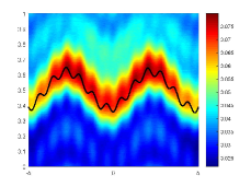
(a) $k_{p}=5.20,\;k_{s}=9$

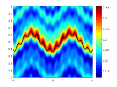
(b) $k_{p}=8.66,\;k_{s}=15$

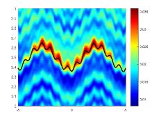
(c) $k_{p}=11.55,\;k_{s}=20$

Fig. 2: Reconstruction of the rough surface in Example 1 at different wave numbers.

Example 2. This example compares the reconstructed results with different measurement places. The exact rough surface $S$ is given by

$$f(x_{1})=0.5+0.1e^{-25(0.15x_{1}-0.5)^{2}}+0.2e^{-49(0.15x_{1}+0.6)^{2}}-0.25e^{-4x_{1}^{2}}.$$

The wave numbers are set to be $k_{p}=8.66,\;k_{s}=15$, and the noise level of the near-field Cauchy data is 20%. Fig. 3 shows that the reconstructed result is getting better if both the measurement line segment $T_{H,A}$ is getting closer to the rough surface and its length $2A$ is getting longer.

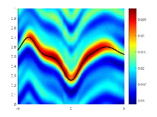
(a) $\{(x_{1},2)|\;|x_{1}|\leq 7.5\}$

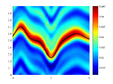
(b) $\{(x_{1},2)|\;|x_{1}|\leq 10\}$

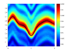
(c) $\{(x_{1},2)|\;|x_{1}|\leq 15\}$

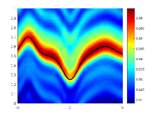
(d) $\{(x_{1},1.2)|\;|x_{1}|\leq 10\}$

(e) $\{(x_{1},2)|\;|x_{1}|\leq 10\}$

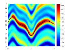
(f) $\{(x_{1},4)|\;|x_{1}|\leq 10\}$

Fig. 3: Reconstruction of the rough surface in Example 2 with different measurement places. Top row (from left to right): the imaging results for the cases when the Cauchy data are measured on $\{(x_{1},2)|\;|x_{1}|\leq 7.5\}$, $\{(x_{1},2)|\;|x_{1}|\leq 10\}$ and $\{(x_{1},2)|\;|x_{1}|\leq 15\}$, respectively. Bottom row (from left to right): the imaging results for the cases when the Cauchy data are measured on $\{(x_{1},1.2)|\;|x_{1}|\leq 10\}$, $\{(x_{1},2)|\;|x_{1}|\leq 10\}$ and $\{(x_{1},4)|\;|x_{1}|\leq 10\}$, respectively.

Example 3. This example presents the reconstructed results with different noise levels. The exact rough surface $S$ is given by

$$f(x_{1})=0.5+0.1\sin(\pi x_{1})+0.1\sin(0.5\pi x_{1}).$$

The near-field Cauchy data are measured on $T_{H,A}$ with $H=2,~{}A=20$, and the wave numbers are set to be $k_{p}=8.66,\;k_{s}=15$. Figure 4 presents the reconstructed results from data without noise, with 20% noise and with 40% noise, respectively. It can be seen that our imaging method is very robust to the noise in the data.

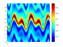
(a) No noise

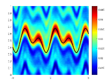
(b) 20% noise

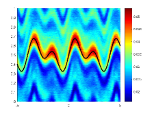
(c) 40% noise

Fig. 4: Imaging results of the rough surface from data with different noise levels.

The above numerical examples illustrate that the direct imaging method gives an accurate and stable reconstruction of the unbounded rough surface and that the imaging method is robust to noise in the measurement data.

5 Conclusion

This paper proposed a novel direct imaging method for inverse elastic scattering problems by an unbounded rigid rough surface from the scattered near-field Cauchy data measured on a horizontal straight line segment at a finite distance above the rough surface. The imaging method can reconstruct the rough surface through computing the inner products of the measured data and the fundamental solution to the Navier equation and thus is very fast. Numerical experiments have been carried out to show that the reconstruction is accurate, stable and robust to noise. The imaging method can be extended to many other cases such as inverse electromagnetic scattering problems by unbounded rough surfaces. Progress in this direction will be reported in the future.

Appendix

The following two lemmas are used to prove the reciprocity relation Lemma 8.

Lemma 10.

Let $T_{b}:=\{x=(x_{1},x_{2})\;|\;x_{1}\in{\mathbb{R}},x_{2}=b\}$ be a horizontal line above the rough surface $S$. Then for the total fields ${\bm{u}}(z;{x},\bm{p})$ and ${\bm{u}}(z;{y},\bm{q})$ corresponding to the incident point sources ${\bm{u}}^{i}(z;x,\bm{p}):=\Gamma(z;x)\bm{p}$ and ${\bm{u}}^{i}(z;y,\bm{q}):=\Gamma(z;y)\bm{q}$, $x,y\in\Omega$ with ${\bm{p}},{\bm{q}}\in{\mathbb{R}}^{2}$, we have

$$\int_{T_{b}}\left[({\bm{P}\bm{u}})(z;x,{\bm{p}})\cdot{\bm{u}}(z;y,\bm{q})-({\bm{P}\bm{u}})(z;y,\bm{q})\cdot{\bm{u}}(z;x,\bm{p})\right]ds(z)=0.$$ (.1)

Proof.

Define the Lamé potentials

$$\Psi_{p}:=-\frac{1}{k_{p}^{2}}\text{div}~{}{\bm{u}}\quad\text{and}\quad\Psi_{s}:=-\frac{1}{k_{s}^{2}}\text{div}~{}{\bm{u}}.$$

Then, by [3, Lemma 2.2] and [12, equation(29)] we get

$${\bm{u}}(z_{1},z_{2}) = \frac{i}{2\pi}\int_{-\infty}^{+\infty}\left(\begin{matrix}\xi\\ \sqrt{k^{2}_{p}-\xi^{2}}\end{matrix}\right)e^{iz_{1}\xi+i(z_{2}-h)\sqrt{k_{p}^{2}-\xi^{2}}}\hat{\Psi}_{p,h}(\xi)d\xi$$ (.2)

$$+\frac{i}{2\pi}\int_{-\infty}^{+\infty}\left(\begin{matrix}\sqrt{k_{s}^{2}-\xi^{2}}\\ -\xi\end{matrix}\right)e^{iz_{1}\xi+i(z_{2}-h)\sqrt{k_{s}^{2}-\xi^{2}}}\hat{\Psi}_{s,h}(\xi)d\xi,\quad z_{2}>h,\;$$

where $\hat{\Psi}_{p,h}(\xi):=(\mathscr{F}\Psi_{p})(\xi,h)$ and $\hat{\Psi}_{s,h}(\xi):=(\mathscr{F}\Psi_{s})(\xi,h)$ denote the Fourier transform of $\Psi_{p}$ and $\Psi_{s}$ on $\Gamma_{h}:=\{z=(z_{1},z_{2})\;|\;z_{1}\in{\mathbb{R}},\,z_{2}=h\}$ with respect to $z_{1}$, respectively. It follows from the angular spectrum representation (.2) that

$$(\mathscr{F}{\bm{u}})(\xi,z_{2}) = i\left(\begin{matrix}\xi\\ \sqrt{k^{2}_{p}-\xi^{2}}\end{matrix}\right)e^{i(z_{2}-h)\sqrt{k_{p}^{2}-\xi^{2}}}\hat{\Psi}_{p,h}(\xi)$$ (.3)

$$+i\left(\begin{matrix}\sqrt{k_{s}^{2}-\xi^{2}}\\ -\xi\end{matrix}\right)e^{i(z_{2}-h)\sqrt{k_{s}^{2}-\xi^{2}}}\hat{\Psi}_{s,h}(\xi).$$

Using (2.4) and a straight calculation gives

$$(\mathscr{F}[{\bm{P}\bm{u}}])(\xi,z_{2}) = -(\mu+\tilde{\mu})\sqrt{k_{p}^{2}-\xi^{2}}\left(\begin{matrix}\xi\\ \sqrt{k^{2}_{p}-\xi^{2}}\end{matrix}\right)e^{i(z_{2}-h)\sqrt{k_{p}^{2}-\xi^{2}}}\hat{\Psi}_{p,h}(\xi)$$

$$-\tilde{\lambda}k^{2}_{p}\left(\begin{matrix}0\\ 1\end{matrix}\right)e^{i(z_{2}-h)\sqrt{k_{p}^{2}-\xi^{2}}}\hat{\Psi}_{p,h}(\xi)$$

$$-(\mu+\tilde{\mu})\sqrt{k_{s}^{2}-\xi^{2}}\left(\begin{matrix}\sqrt{k_{s}^{2}-\xi^{2}}\\ -\xi\end{matrix}\right)e^{i(z_{2}-h)\sqrt{k_{s}^{2}-\xi^{2}}}\hat{\Psi}_{s,h}(\xi)$$

$$+\tilde{\mu}k^{2}_{s}\left(\begin{matrix}1\\ 0\end{matrix}\right)e^{i(z_{2}-h)\sqrt{k_{s}^{2}-\xi^{2}}}\hat{\Psi}_{s,h}(\xi).$$ (.4)

By Parseval’s formula and the fact that $\overline{(\mathscr{F}\overline{\bm{u}})(\xi)}=({\mathscr{F}}{\bm{u}})(-\xi)$, we deduce

$$\int_{T_{b}}\left[({\bm{P}\bm{u}})({z};{x},\bm{p})\cdot{\bm{u}}({z};{y},\bm{q})-({\bm{P}\bm{u}})({z};{y},\bm{q})\cdot{\bm{u}}({z};{x},\bm{p})\right]ds(z)$$

$$\quad=(2\pi)^{-1}\int_{-\infty}^{+\infty}\left[(\mathscr{F}[{\bm{P}\bm{u}}])((\xi,b);x,\bm{p})\overline{(\mathscr{F}\overline{\bm{u}})}((\xi,b);y,\bm{q})\right.$$

$$\qquad\;\;\left.-(\mathscr{F}[{\bm{P}\bm{u}}])((\xi,b);{y},\bm{q})\overline{(\mathscr{F}\overline{\bm{u}})}((\xi,b);x,\bm{p})\right]d\xi$$

$$\quad=(2\pi)^{-1}\int_{-\infty}^{+\infty}\left[(\mathscr{F}[{\bm{P}\bm{u}}])((\xi,b);{x},\bm{p})(\mathscr{F}{\bm{u}})((-\xi,b);{y},\bm{q})\right.$$

$$\qquad\;\;\left.-(\mathscr{F}[{\bm{P}\bm{u}}])((\xi,b);{y},\bm{q})({\mathscr{F}}{\bm{u}})((-\xi,b);{x},\bm{p})\right]d\xi,\;\;\;b>h.$$ (.5)

Insert (.3) and (.4) into (.5) to get

$$\int_{T_{b}}\left[({\bm{P}\bm{u}})({z};{x},\bm{p})\cdot{\bm{u}}({z};{y},\bm{q})-({\bm{P}\bm{u}})({z};{y},\bm{q})\cdot{\bm{u}}({z};{x},\bm{p})\right]ds(z):=\sum_{j=1}^{8}I_{j},$$

where

$$I_{1} = -i(\mu+\tilde{\mu})\int_{-\infty}^{+\infty}\sqrt{k_{p}^{2}-\xi^{2}}(k^{2}_{p}-2\xi^{2})e^{2i(b-h)\sqrt{k_{p}^{2}-\xi^{2}}}\left[\hat{\Psi}_{p,h,xp}(\xi)\hat{\Psi}_{p,h,yq}(-\xi)\right.$$

$$\quad\left.-\hat{\Psi}_{p,h,yq}(\xi)\hat{\Psi}_{p,h,xp}(-\xi)\right]d\xi,$$

$$I_{2} = -i(\mu+\tilde{\mu})\int_{-\infty}^{+\infty}\sqrt{k_{s}^{2}-\xi^{2}}(k^{2}_{s}-2\xi^{2})e^{2i(b-h)\sqrt{k_{s}^{2}-\xi^{2}}}\left[\hat{\Psi}_{s,h,xp}(\xi)\hat{\Psi}_{s,h,yq}(-\xi)\right.$$

$$\quad\left.-\hat{\Psi}_{s,h,yq}(\xi)\hat{\Psi}_{s,h,xp}(-\xi)\right]d\xi,$$

$$I_{3} = -i(\mu+\tilde{\mu})\int_{-\infty}^{+\infty}\xi\sqrt{k_{p}^{2}-\xi^{2}}(\sqrt{k^{2}_{p}-\xi^{2}}+\sqrt{k^{2}_{s}-\xi^{2}})e^{i(b-h)(\sqrt{k^{2}_{p}-\xi^{2}}+\sqrt{k^{2}_{s}-\xi^{2}})}$$

$$\qquad\;\cdot\left[\hat{\Psi}_{p,h,xp}(\xi)\hat{\Psi}_{s,h,yq}(-\xi)-\hat{\Psi}_{p,h,yq}(\xi)\hat{\Psi}_{s,h,xp}(-\xi)\right]d\xi,$$

$$I_{4} = i(\mu+\tilde{\mu})\int_{-\infty}^{+\infty}\xi\sqrt{k_{s}^{2}-\xi^{2}}(\sqrt{k^{2}_{p}-\xi^{2}}+\sqrt{k^{2}_{s}-\xi^{2}})e^{i(b-h)(\sqrt{k^{2}_{p}-\xi^{2}}+\sqrt{k^{2}_{s}-\xi^{2}})}$$

$$\qquad\;\cdot\left[\hat{\Psi}_{s,h,xp}(\xi)\hat{\Psi}_{p,h,yq}(-\xi)-\hat{\Psi}_{s,h,yq}(\xi)\hat{\Psi}_{p,h,xp}(-\xi)\right]d\xi,$$

$$I_{5} = -i\tilde{\lambda}k^{2}_{p}\int_{-\infty}^{+\infty}\sqrt{k_{p}^{2}-\xi^{2}}e^{2i(b-h)\sqrt{k_{p}^{2}-\xi^{2}}}$$

$$\qquad\;\cdot\left[\hat{\Psi}_{p,h,xp}(\xi)\hat{\Psi}_{p,h,yq}(-\xi)-\hat{\Psi}_{p,h,yq}(\xi)\hat{\Psi}_{p,h,xp}(-\xi)\right]d\xi,$$

$$I_{6} = i\tilde{\mu}k^{2}_{s}\int_{-\infty}^{+\infty}\sqrt{k_{s}^{2}-\xi^{2}}e^{2i(b-h)\sqrt{k_{s}^{2}-\xi^{2}}}$$

$$\qquad\;\cdot\left[\hat{\Psi}_{s,h,xp}(\xi)\hat{\Psi}_{s,h,yq}(-\xi)-\hat{\Psi}_{s,h,yq}(\xi)\hat{\Psi}_{s,h,xp}(-\xi)\right]d\xi,$$

$$I_{7} = -i\tilde{\lambda}k^{2}_{p}\int_{-\infty}^{+\infty}\xi e^{i(b-h)\left(\sqrt{k^{2}_{p}-\xi^{2}}+\sqrt{k^{2}_{s}-\xi^{2}}\right)}$$

$$\qquad\;\cdot\left[\hat{\Psi}_{p,h,xp}(\xi)\hat{\Psi}_{s,h,yq}(-\xi)-\hat{\Psi}_{p,h,yq}(\xi)\hat{\Psi}_{s,h,xp}(-\xi)\right]d\xi,$$

$$I_{8} = -i\tilde{\mu}k^{2}_{s}\int_{-\infty}^{+\infty}\xi e^{i(b-h)\left(\sqrt{k^{2}_{p}-\xi^{2}}+\sqrt{k^{2}_{s}-\xi^{2}}\right)}$$

$$\qquad\;\cdot\left[\hat{\Psi}_{s,h,xp}(\xi)\hat{\Psi}_{p,h,yq}(-\xi)-\hat{\Psi}_{s,h,yq}(\xi)\hat{\Psi}_{p,h,xp}(-\xi)\right]d\xi.$$

From the fact that

$$\int_{-\infty}^{+\infty}a(\xi)f(\xi)g(-\xi)d\xi = \int_{-\infty}^{+\infty}a(\xi)f(-\xi)g(\xi)d\xi\quad\mbox{if $a$ is an even function},$$

$$\int_{-\infty}^{+\infty}b(\xi)f(\xi)g(-\xi)d\xi = -\int_{-\infty}^{+\infty}b(\xi)f(-\xi)g(\xi)d\xi\quad\mbox{if $b$ is an odd function},$$

we obtain that $I_{1}=I_{2}=I_{5}=I_{6}=0$ and

$$I_{3}+I_{4}+I_{7}+I_{8} = \int_{-\infty}^{+\infty}i[(\mu+\tilde{\mu})(k_{s}^{2}-k_{p}^{2})-\tilde{\lambda}k_{p}^{2}-\tilde{\mu}k^{2}_{s}]\xi e^{i(b-h)(\sqrt{k^{2}_{p}-\xi^{2}}+\sqrt{k^{2}_{s}-\xi^{2}})}$$

$$\qquad\;\cdot\left[\hat{\Psi}_{s,h,xp}(\xi)\hat{\Psi}_{p,h,yq}(-\xi)-\hat{\Psi}_{s,h,yq}(\xi)\hat{\Psi}_{p,h,xp}(-\xi)\right]d\xi.$$

Since $\mu+\lambda=\tilde{\mu}+\tilde{\lambda}$, $k_{s}^{2}=\omega^{2}/\mu$ and $k^{2}_{p}=\omega^{2}/(2\mu+\lambda)$, then $I_{3}+I_{4}+I_{7}+I_{8}=0$. The required equation (.1) thus follows. The lemma is thus proved. ∎

Lemma 11.

Let $B_{\varepsilon}({x}):=\{z\in{\mathbb{R}}^{2}\;|\;|z-x|<\varepsilon\}$ be a ball centered at $x$ with radius $\varepsilon$. Then, for any total field $\bm{u}$ of the scattering problem corresponding to the incident point source ${\bm{u}}^{i}(z;x,\bm{p})=\Gamma(z,x)\bm{p}$ with ${\bm{p}}\in{\mathbb{R}}^{2}$ we have

$${\bm{u}}(x)\cdot{\bm{p}}=\int_{\partial B_{\varepsilon}(x)}\left[({\bm{P}\bm{u}})(z)\cdot{\bm{u}}^{i}(z;x,\bm{p})-{\bm{u}}(z)\cdot({\bm{P}\bm{u}}^{i})(z;x,\bm{p})\right]ds(z).$$ (.6)

Proof.

By a direct calculation it can be derived that on $\partial B_{\varepsilon}(x)$,

$$\Gamma(z,x):=I_{1}+I_{2}+I_{3}+I_{4},$$

where

$$I_{1} = \frac{i}{4\omega^{2}}\left(k_{p}^{2}H^{(1)}_{0}(k_{p}\varepsilon)-k_{s}^{2}H^{(1)}_{0}(k_{s}\varepsilon)\right)\hat{R}\otimes\hat{R},$$

$$I_{2} = -\frac{i}{2\omega^{2}\varepsilon}\left(k_{p}H^{(1)}_{1}(k_{p}\varepsilon)-k_{s}H^{(1)}_{1}(k_{s}\varepsilon)\right)\hat{R}\otimes\hat{R},$$

$$I_{3} = \frac{i}{4\omega^{2}\varepsilon}\left(k_{p}H^{(1)}_{1}(k_{p}\varepsilon)-k_{s}H^{(1)}_{1}(k_{s}\varepsilon)\right){I},$$

$$I_{4} = \frac{i}{4\mu}H^{(1)}_{0}(k_{s}\varepsilon){I}.$$

Here, $R=z-x:=(R_{1},R_{2}),~{}|z-x|=\varepsilon$ and $\hat{R}=(z-x)/|z-x|$.

By the definition of the generalised stress operator ${\bm{P}}$ in (2.4), and setting $R_{\perp}=(R_{2},-R_{1})$, we have

$${\bm{P}}(I_{1}\bm{q}) = \frac{i}{4\omega^{2}}\left[(\lambda+2\mu)\left(k_{p}^{3}H^{(1)^{\prime}}_{0}(k_{p}\varepsilon)-k_{s}^{3}H^{(1)^{\prime}}_{0}(k_{s}\varepsilon)\right)\right.$$

$$\qquad\;\;\left.+\frac{\lambda}{\varepsilon}\left(k_{p}^{2}H^{(1)}_{0}(k_{p}\varepsilon)-k_{s}^{2}H^{(1)}_{0}(k_{s}\varepsilon)\right)\right]\hat{R}\otimes\hat{R}\bm{q}$$

$$\qquad\;\;+\frac{i}{4\omega^{2}}\frac{\mu}{\varepsilon}\left(k_{p}^{2}H^{(1)}_{0}(k_{p}\varepsilon)-k_{s}^{2}H^{(1)}_{0}(k_{s}\varepsilon)\right)\hat{R_{\perp}}\otimes\hat{R_{\perp}}\bm{q},$$

$${\bm{P}}(I_{2}\bm{q}) = -\frac{i}{2\omega^{2}}\left[\frac{\lambda+2\mu}{\varepsilon}\left(k_{p}^{2}H^{(1)^{\prime}}_{1}(k_{p}\varepsilon)-k_{s}^{2}H^{(1)^{\prime}}_{1}(k_{s}\varepsilon)\right)\right.$$

$$\qquad\;\;\left.-\frac{2\mu}{\varepsilon^{2}}\left(k_{p}H^{(1)}_{1}(k_{p}\varepsilon)-k_{s}H^{(1)}_{1}(k_{s}\varepsilon)\right)\right]\hat{R}\otimes\hat{R}\bm{q}$$

$$\qquad\;\;-\frac{i}{2\omega^{2}}\frac{\mu}{\varepsilon^{2}}\left(k_{p}H^{(1)}_{1}(k_{p}\varepsilon)-k_{s}H^{(1)}_{1}(k_{s}\varepsilon)\right)\hat{R_{\perp}}\otimes\hat{R_{\perp}}\bm{q},$$

$${\bm{P}}(I_{3}\bm{q}) = \frac{i}{4\omega^{2}}\left[\left(\frac{k_{p}^{2}}{\varepsilon}H^{(1)^{\prime}}_{1}(k_{p}\varepsilon)-\frac{k_{p}}{\varepsilon^{2}}H^{(1)}_{1}(k_{p}\varepsilon)\right)\right.$$

$$\qquad\;\;\;\left.-\left(\frac{k_{s}^{2}}{\varepsilon}H^{(1)^{\prime}}_{1}(k_{s}\varepsilon)-\frac{k_{s}}{\varepsilon^{2}}H^{(1)}_{1}(k_{s}\varepsilon)\right)\right]\left[(\lambda+\mu)\hat{R}\otimes\hat{R}+\mu I\right]\bm{q},$$

$${\bm{P}}(I_{4}\bm{q}) = \frac{i}{4\mu}k_{s}H^{(1)^{\prime}}_{0}(k_{s}\varepsilon)\left[(\lambda+\mu)\hat{R}\otimes\hat{R}+\mu I\right]\bm{q}.$$

Thus it follows that

$${\bm{P}}(\Gamma(z,{x})\bm{q}) := -\frac{i}{4}k_{s}H^{(1)}_{1}(k_{s}\varepsilon)I+\frac{i\mu}{4\omega^{2}\varepsilon}\left[\frac{2}{\varepsilon}\left(k_{p}H^{(1)}_{1}(k_{p}\varepsilon)-k_{s}H^{(1)}_{1}(k_{s}\varepsilon)\right)\right.$$

$$\qquad\;\left.-\left(k_{p}^{2}H^{(1)}_{0}(k_{p}\varepsilon)-k_{s}^{2}H^{(1)}_{0}(k_{s}\varepsilon)\right)\right](\hat{R_{\perp}}\otimes\hat{R_{\perp}}-\hat{R}\otimes\hat{R})\bm{q}.$$

Noting that

$$\frac{i}{4}H^{(1)}_{0}(k_{\beta}\varepsilon) \approx \frac{1}{2\pi}\ln\frac{1}{\varepsilon}+\frac{i}{4}-\frac{1}{2\pi}\ln\frac{k_{\beta}}{2}-\frac{C}{2\pi}\quad\mbox{as}\;\varepsilon\rightarrow 0,$$

$$H^{(1)}_{m}(k_{\beta}\varepsilon) \approx \frac{(k_{\beta}\varepsilon)^{m}}{2^{m}m!}-i\frac{2^{m}(m-1)!}{\pi(k_{\beta}\varepsilon)^{m}},\quad m=1,2,\quad\mbox{as}\;\varepsilon\rightarrow 0,$$

where $C$ denotes Euler’s constant, we deduce that

$$\lim_{\varepsilon\rightarrow 0}2\pi\varepsilon\Gamma({{z},x}) = \lim_{\varepsilon\rightarrow 0}\varepsilon\left[\frac{k_{p}^{2}}{\omega^{2}}\left(\ln\frac{1}{\varepsilon}-\ln\frac{k_{p}}{2}-C\right)-\frac{k_{s}^{2}}{\omega^{2}}\left(\ln\frac{1}{\varepsilon}-\ln\frac{k_{s}}{2}-C\right)\right]\hat{R}\otimes\hat{R}$$

$$+\lim_{\varepsilon\rightarrow 0}\varepsilon\left[\frac{i\pi(k_{p}^{2}-k_{s}^{2})}{4\omega^{2}}+\frac{k_{s}^{2}}{\omega^{2}}\left(\ln\frac{1}{\varepsilon}+\frac{i\pi}{2}-\ln\frac{k_{s}}{2}-C\right)\right]I=0,$$

$$\lim_{\varepsilon\rightarrow 0}2\pi\varepsilon{\bm{P}}(\Gamma({z},{x})\bm{q}) = \lim_{\varepsilon\rightarrow 0}\left[\left(-\frac{i\pi k_{s}^{2}\varepsilon^{2}}{4}+1\right)I+\frac{i\pi\mu\varepsilon^{2}(k_{p}^{2}-k_{s}^{2})}{8\omega^{2}}(\hat{R_{\perp}}\otimes\hat{R_{\perp}}-\hat{R}\otimes\hat{R})\bm{q}\right]$$

$$= I.$$

The above two equations and the mean value theorem then imply the required equation (.6). ∎

References

• [1] K. Aki and P. Richards, Quantitative Seismology, Vol. 1, W.H. Freeman & Co., San Francisco, 1980.
• [2] H. Ammari, E. Bretin, J. Garnier, H. Kang, H. Lee and A. Wahab, Mathematical Methods in Elasticity Imaging, Princeton University Press, 2015.
• [3] T. Arens, The Scattering of Elastic Waves by Rough Surfaces, PhD Thesis, Brunel University, UK, 2000.
• [4] T. Arens, Uniqueness for elastic wave scattering by rough surfaces, SIAM J. Math. Anal. 33 (2001), 461-476.
• [5] T. Arens, Existence of solution in elastic wave scattering by unbounded rough surfaces, Math. Methods Appl. Sci. 25 (2002), 507-528.
• [6] T. Arens, Linear sampling method for 2D inverse elastic wave scattering, Inverse Problems 17 (2001), 1445-1464.
• [7] T. Arens and A. Kirsch, The factorization method in inverse scattering from periodic structures, Inverse Problems 19 (2003), 1195-1211.
• [8] K. Baganas, B.B. Guzina and A. Charalambopoulos, A linear sampling method for the inverse transmission problem in near-field elastodynamics, Inverse Problems 22 (2006), 1835-1853.
• [9] G. Bao and P. Li, Near-field imaging of infinite rough surfaces, SIAM J. Appl. Math. 73 (2013), 2162-2187.
• [10] G. Bao and P. Li, Near-field imaging of infinite rough surfaces in dielectric media, SIAM J. Imaging Sci. 7 (2014), 867-899.
• [11] C. Burkard and R. Potthast, A time-domain probe method for three-dimensional rough surface reconstructions, Inverse Problems and Imaging 3 (2009), 259-274.
• [12] S.N. Chandler-Wilde, The impedance boundary value problem for the Helmholtz equation in a half-plane, Math. Meth. Appl. Sci. 20 (1997), 813-840.
• [13] J. Chen, Z. Chen and G. Huang, Reverse time migration for extended obstacles: acoustic waves, Inverse Problems 29 (2013) 085005.
• [14] Z. Chen and G. Huang, Reverse time migration for extended obstacles: elastic waves (in Chinese), Science in China A: Math. 45 (2015), 1103-1114.
• [15] D. Colton and R. Kress, Inverse Acoustic and Electromagnetic Scattering Theory (3rd Edition), Springer, New York, 2013.
• [16] A. Charalambopoulos, A. Kirsch, K. A. Anagnostopoulos, D. Gintides and K. Kiriaki, The factorization method in inverse elastic scattering from penetrable bodies, Inverse Problems 23 (2007), 27-51.
• [17] S.N. Chandler-Widle and C. Lines, A time domain point source method for inverse scattering by rough surfaces, Computing 75 (2005), 157-180.
• [18] J. Elschner and G. Hu, Elastic scattering by unbounded rough surfaces, SIAM J. Math. Anal. 44 (2012), 4101-4127.
• [19] J. Elschner and G. Hu, Elastic scattering by unbounded rough surfaces: solvability in weighted Sobolev spaces, Appl. Anal. 94 (2015), 251-278.
• [20] J. Elschner and G. Hu, An optimization method in inverse elastic scattering for one-dimensional grating profiles, Commun. Comput. Phys. 12 (2012), 1434-1460.
• [21] G. Hu, Y. Lu and B. Zhang, The factorization method for inverse elastic scattering from periodic structures, Inverse Problems 29 (2013) 115005 (25pp).
• [22] G. Hu, A. Kirsch and T. Yin, Factorization method in inverse interaction problems with bi-periodic interfaces between acoustic and elastic waves, Inverse Probl. Imaging 10 (2016), 103-129.
• [23] K. Ito, B. Jin and J. Zou, A direct sampling method to an inverse medium scattering problem, Inverse Problems 28 (2012) 025003.
• [24] J. Li, H. Liu, Z. Shang and H. Sun, Two single-shot methods for locating multiple electromagnetic scatterers, SIAM J. Appl. Math. 73 (2013), 1721-1746.
• [25] J. Li, H. Liu and J. Zou, Locating multiple multiscale acoustic scatterers, Multiscale Model. Simul. 12 (2014), 927-952.
• [26] J. Li and G. Sun, A nonlinear integral equation method for the inverse scattering problem by sound-soft rough surfaces, Inverse Probl. Sci. Enging. 23 (2015), 557-577.
• [27] J. Li, G. Sun and B. Zhang, The Kirsch-Kress method for inverse scattering by infinite locally rough interfaces, Appl. Anal. 96 (2017), 85-107.
• [28] P. Li and Y. Wang, Near-field imaging of small perturbed obstacles for elastic waves, Inverse Problems 31 (2015) 085010
• [29] P. Li, Y. Wang and Y. Zhao, Inverse elastic surface scattering with near-field data, Inverse Problems 31 (2015) 035009.
• [30] P. Li, Y. Wang, Z. Wang and Y. Zhao, Inverse obstacle scattering for elastic waves, Inverse Problems 32 (2016) 115018.
• [31] P. Li, Y. Wang and Y. Zhao, Near-field imaging of biperiodic surfaces for elastic waves, J. Comput. Phy. 324 (2016), 1-23.
• [32] X. Liu, J. Li, B. Zhang and H. Zhang, A Nyström method for elastic wave scattering by an unbounded rough surface, in preparation, 2018.
• [33] X. Liu, B. Zhang and H. Zhang, A direct imaging method for inverse scattering by an unbounded rough surface, accepted by SIAM J. Imaging Sci., arXiv:1801.06280v1, 2018.
• [34] X. Liu, A novel sampling method for multiple multiscale targets from scattering amplitudes at a fixed frequency, Inverse Problems 33 (2017) 085011
• [35] F.S. Nintcheu and B.B. Guzina, A linear sampling method for near-field inverse problems in elastodynamics, Inverse Problems 20 (2004), 713-736.
• [36] R. Potthast, A study on orthogonality sampling, Inverse Problems 26 (2010) 074015.
• [37] J. Yang, B. Zhang and R. Zhang, A sampling method for the inverse transmission problem for periodic media. Inverse Problems 28 (2012) 035004.
• [38] J. Yang, B. Zhang and R. Zhang, Reconstruction of penetrable grating profiles, Inverse Probl. Imaging 7 (2013), 1393-1407.
• [39] J. Yang, B. Zhang and R. Zhang, Near-field imaging of periodic interfaces in multilayered media, Inverse Problems 32 (2016) 035010.
• [40] T. Yin, G. Hu, L. Xu and B. Zhang, Near-field imaging of obstacles with the factorization method: Fluid-solid interaction, Inverse Problems 32 (2016) 015003.
• [41] H. Zhang and B. Zhang, A novel integral equation for scattering by locally rough surfaces and application to the inverse problem, SIAM J. Appl. Math. 73 (2013), 1811-1829.