Computing Information Quantity as Similarity Measure for Music Classification Task

Abstract

This paper proposes a novel method that can replace compression-based dissimilarity measure (CDM) in composer estimation task. The main features of the proposed method are clarity and scalability. First, since the proposed method is formalized by the information quantity, reproduction of the result is easier compared with the CDM method, where the result depends on a particular compression program. Second, the proposed method has a lower computational complexity in terms of the number of learning data compared with the CDM method. The number of correct results was compared with that of the CDM for the composer estimation task of five composers of 75 piano musical scores. The proposed method performed better than the CDM method that uses the file size compressed by a particular program.

I Introduction

When people listen to music, they can determine many features, such as genre and composer. The genre of music is easy to determine without previous knowledge, but not the composer, even if you have some knowledge. The difficulty depends on what should be estimated. There are some existing studies for such estimation, which are based on machine learning  [1, 2].

The contribution of  [2] implies that the feature that reflects the composer is short note sequence. Since the compression program is a kind of program which captures frequent sequences of data, it may not be suprising if we use a compression program to estimate composer. Actually, there is an interesting research  [3] that uses compression programs for composer estimation. They use the formular called NCD (Normalized Compression Distance). We focus on a similar but different similarity measure called compression-based dissimilarity measure (CDM) [4], which is tested in a wide range of data, not limited to music. Both CDM and NCD are based on the same plinciple. These principle are recently well presented in  [5].

Although a compression program is easy to use, the result depends on the compression program and the behavior is difficult to analyze. Moreover, since the compression is carried out with every known musical score, there is a concern that the amount of calculation becomes enormous when we determine the degree of similarity for a new musical score. In this study, we propose a novel method that is well formalized. The proposed method realized the scalability of a large number of learning data by pre-processing the group of learning data. Finally, the precision of the proposed method was verified to be better than the method where the value of the CDM is determined by the compressed file size.

II Baseline Method

In this section, we will describe baseline CDM method [6] for estimating the composers. This work focuses on the improvement of CDM. They conducted experiments on a very simple system with CDM, but it still performs well for composer estimation task, in order to make the analysis of improvments possible. We have followed this work because we are also interesting in CDM, although we are aiming at replacing CDM with the proposed method, rather than simply improving the CDM. In baseline method, the musical scores are first converted into string representation, where information for sound ’on’ or ’off’ is expressed. The string representation is a long sequence of character ’0’ for ’off’ and character ’1’ for ’on’. The position of each character corresponds to a piano key number $key$ and timing number $time$, where $position=88\times time+key$. The number 88 is the number of keys on a piano. Second, it uses the CDM proposed by Keogh [4] for a pair of musical scores. The CDM is defined as follows:

$${\rm CDM}(x,y) = \frac{C(xy)}{C(x)+C(y)}$$ (1)

where $C(x)$ is the compressed file size of string $x$, and $C(xy)$ is the compressed file size of the concatenation of $x$ and $y$. The value of the CDM shows the dissimilarity between the two strings. The more the patterns shared by the two strings, the smaller the CDM value of the two strings. It is based on the principle that the string has more similar patterns, such as repetitions, if the compressed file size of its concatenated string is smaller based on the assumption that if specific phrases of the composer exist, then he/she used them in other musical scores. The estimation of the composer is based on this concept. This method is based on the study in [6].

It is interesting that the CDM, which is a simple function of a compressed file size, can estimate the composer of musical scores. However, there is an issue of scalability in the CDM. Figure 1 illustrates this issue, where $x$ is the string representation of a musical score of unknown composer, and $a_{1}$ to $a_{15}$ are musical scores of a composer $A$. The CDM is defined as a measure between two musical scores. In a previous study of composer estimation, an unknown musical score was compared with all the known musical scores, then the $k$-nearest neighbor method ($k$-NN) was applied [7] to the result. In general, when an application uses the relationship between two scores, an unknown musical score need to be compared with all the known musical scores. The larger is the number of known scores, the more are the computation time required for one new musical score. This method cannot be scaled up to a large number of known musical scores.

The study in [6] also argues that the compressed file size of string $x$ is the approximation of the information quantity. The study in [6] also proposes to use offsetted compressed file size, where the value of the offset is obtained by observing the behavior of a specific compression program. This method was reported to improve the number of correct estimation significantly. However, the problems of dependency on the compression program and scalability remained the same with the CDM method.

III Proposed Method

In this study, we formed a group of musical scores of the same composer to address the scalability issue. Then, we computed the information quantity based on the probability of substrings of a large string. This large string corresponds to the group. Figure 2 shows how the groups were used. As is in Figure 1, in Figure 2, $x$ is the string representation of a musical score of unknown composer, and $a_{1}$ to $a_{15}$ are musical scores of a composer $A$. The box shows that these scores form a group, and there is one long string representation for one group. The information quantity is then computed using the probability in $a_{1},a_{2},...,a_{15}$, and not the probability in $x$.

Then, we computed the information quantity of an unknown musical score using the method described in the next session. The same process was carried out for the musical scores of the other four composers. We computed the information quantity of the unknown musical score $x$ with the group of each composer. We obtained five information quantities and determined that the composer of $x$ is the one whose string had the least information quantity.

Using the pre-processing, the computation time of information quantity of one music score does not depend on the number of music score in a group. It only depends on the length of music score to judge. Therefore, the number of computations for one unknown musical score is proportional to the number of composers, rather than the number of known musical scores.

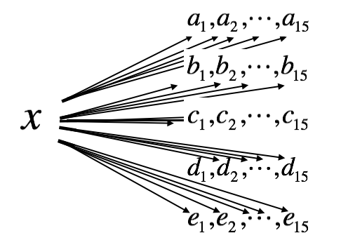
Figure 1: Baseline system and other compression based approaches. When a method uses the relationship between two scores, an unknown musical score need to be compared with all the known musical scores.

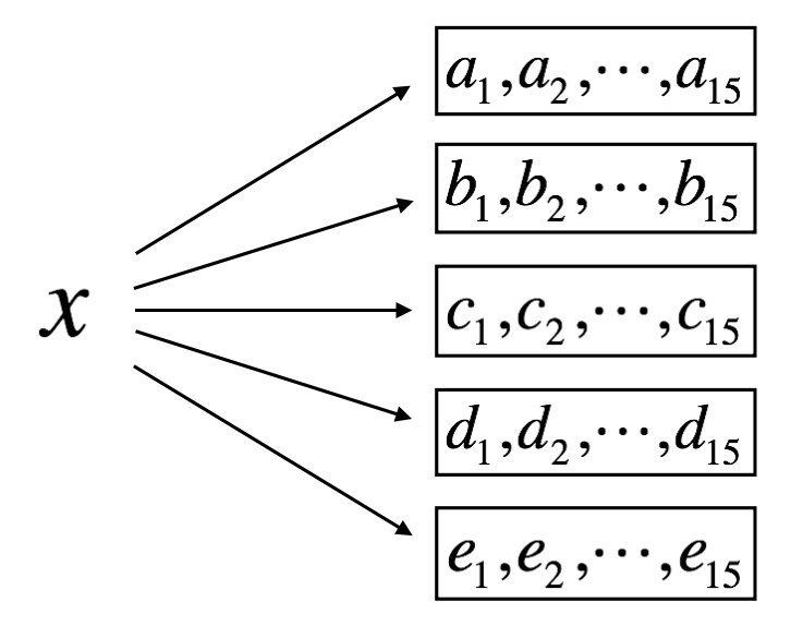
Figure 2: Proposed system or scalable method. By pre-prosessing through all music score in a group. computation time of one music scores not depend the number of scores in group.

IV Information Quantity

In general, we calculate the information quantity of a string from the probabilities of characters in the string. However, we can make a good guess that specified substrings, such as words emerge repeatedly in the real strings. Therefore, in this study the calculation of the information quantity of a string was performed using the emergent probabilities of all substrings.

First, we consider the information quantity of one character. In general, the information quantity of a certain event depends on the occurring probability. Let the emergent probability of a certain character $c$ be $P(c)$, then the information quantity of $c$ is expressed using self-information [8] as follows:

$$I_{c}(c)=-\log_{2}P(c)$$ (2)

Let us consider the information quantity for the case where we treat the character sequence as a string. Let the $i$-th character of a string $S$ with length $N$ be $c_{i}$. The character $c_{i}$ in $S$ is independent of each other. The information quantity $I_{c}(S)$ of $S$ based on the characters is expressed as (3). The expression in (3) indicates that the string information quantity is equal to the total sum of the information quantity of the characters.

$$I_{c}(S) = -\log_{2}(\prod_{i=1}^{N}P(c_{i}))$$ (3)

$$= -\sum_{i=1}^{N}\log_{2}P(c_{i})$$

For the case of the string representation of a musical score, specified substrings, such as motif may emerge repeatedly. Thus, if we assume that a string consists of some subsequences, then the information quantity $I_{s}$ is expressed as (4).

$$I_{s}(S)=\mathop{\rm min}\limits_{\pi_{k}\in\pi(S)}\Bigl{(}-\sum_{t\in\pi_{k}}\log_{2}P(t)\Bigr{)}$$ (4)

where $\pi(S)$ is the set of all possible ways to divide $S$, which includes $2^{N-1}$ ways, and $t$ is a member of divided strings (a substring). More precisely, we divide the strings into finer substrings and calculate the information quantity as the sum of the information quantities of the new divided substrings. The information quantity varies depending on the partition. We should take the minimum quantity because the more are the substrings considered, the less becomes the information quantity of the string. The number of partitions is $2^{N-1}$, where $N$ is the length of the string. Although this is a large number, the minimum value is easily obtained in $\mathcal{O}(N^{2})$, when a dynamic programming is used.

To implement a program that obtains $I_{s}(S)$, we require a module to compute $P(t)$, where $t$ can be all substrings of the given large string. An efficient data structure, called suffix array, can be used to obtain the frequency of any substring [9]. Using this data structure, whose size is proportional to size of the large string, we can obtain the frequency of a substring $t$ in the large string efficiently. We used suffix array in the program implemented in this study. There is also a more efficient data structure called suffix tree [10]. Furthermore, there is a good algorithm that can construct suffix tree in $\mathcal{O}(N)$ time complexities, and $\mathcal{O}(1)$ time complexities to obtain the frequency of a substring using the suffix tree. Maximum Likelihood Estimator (MLE) is usually used to estimate the probability from the frequency. We use MLE but we use $frequency-1$ rather than $frequency$ in order to make the computed value stable.

V Computational Complexity

Let us examine by how much the computational complexity is reduced by the proposed method compared with the existing method.

Let $l$ be the average length of a string representation of a musical score. Let $c$ be the number of composers. Let $g$ be the average number of musical scores in one group. Let $n$ be the number of unknown musical scores.

First, the computational complexity to compress a string representation of musical score is proportional to the length of the string. Thus:

$$T_{compression}=\mathcal{O}(l)$$ (5)

To estimate the composer of one musical score using CDM, we need to compute $g\times c$ compression:

$$T_{CDM-ONE}=\mathcal{O}(l\times g\times c))$$ (6)

When there are many musical scores, we need to repeat the above operation for each $n$ musical scores.

$$T_{CDM}=\mathcal{O}(n\times l\times g\times c)$$ (7)

To compute one information quantity in Figure 2, we need to compute two things: the pre-processing of the groups and to obtain the minimum of the considered partition.

$$T_{information-quantity}=\mathcal{O}(g\times l+l^{2})$$ (8)

To estimate the composer of one musical score using the proposed method, we need to compute the information quantity $c$ times.

$$T_{Proposed-ONE}=\mathcal{O}(c\times g\times l+c\times l^{2})$$ (9)

When there are many musical scores, we only require one pre-processing operation. This is the reason why the proposed method is scalable.

$$T_{Proposed}=\mathcal{O}(c\times g\times l+n\times c\times l^{2})$$ (10)

Both the complexity of $T_{CDM}$ and the $T_{Proposed}$ are proportional to $c$. There is no difference with respect to $c$. When $n$ is large, the computational complexity of the proposed method is independent of $g$, while that of the CDM is multiplied by $g$. This means that when the number of musical scores for each composer increases, the computational complexity of the proposed method becomes smaller than CDM method.

The proposed method has a complexity that is proportional to the square of the length of the unknown musical score, while that of the CDM method is proportional to the length. This is because the proposed method considers all substrings, while the compression program only considers some subsets of the substrings. As a result, the proposed method requires a large value of $g$ when the $l$ is large.

VI Evaluation

For the evaluation, the result can be much better than it should be if we include the same musical score as $x$ in some of the known musical scores. Therefore, we have to change our setting from Figure 2 into Figure 3 to measure the correctness of the methods. The musical score in question should be intentionally excluded from the set of known musical scores. In the CDM method, the CDM between the same musical scores was not computed using the one-leave-out method. Figure 3 corresponds to this approach. In doing so, we need to pre-process many times, and this is only for the evaluation, and not the actual estimation.

In Figure 3, A, B, C, D, and E indicate the composers and $a_{1},\cdots,a_{15}$ denote the musical scores of composer A. When we need to estimate the composer of $a_{1}$, we remove $a_{1}$ from the group of composer A, and create a new group data of the remaining musical scores. Then, we calculate the information quantities of $a_{1}$ with each of the five grouping data. We estimate that the composer of $a_{1}$ is the one whose string attains the least information quantity. Then, we determine the estimation from the information that the composer of $a_{1}$ is A. This information is used only for determining the correctness of the estimation.

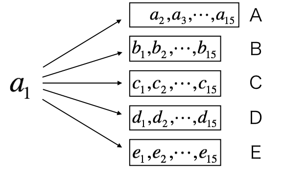
Figure 3: For the evaluation, the result can be much better than it should be if we include the same musical score in some of the known musical scores. Therefore, the musical score in question should be intentionally excluded from the set of known musical scores for evaluation. This corresponds to one-leave-out method.

A summary of the total correct results is presented in TABLE I. In the estimations of 75 musical scores, the proposed method yielded 55 correct results. Since the task was to select one composer out of five composers, a random choice can achieve 20% correct answers. Our method achieved more than 70% correct answers. This suggests that the proposed method can estimate the composer. Unlike the CDM, the proposed method is formalized as the estimation of information quantity, and is not dependent on a particular compression program. Therefore, reproduction of the result should be much easier than the CDM.

TABLE I: Summary

		System
		Proposed	CDM	Offseted CDM
	Bach	9	10	11
	Chopin	9	5	6
Group	Debussy	14	11	12
	Mozart	13	7	11
	Satie	10	8	8
	Total	55	41	48

As presented in TABLE I, the proposed method yielded more correct results than previous methods. We performed the McNemar’s test of the proposed method with the original CDM and with offsetted CDM [6]. As presented in table TABLE II, the proposed method performed better than the CDM with a significance of $\alpha<0.01$, although we could not achieve the statistical significance in TABLE III.

Since offsetted CDM [6] aimed to obtain a more precise value of the information quantity rather than the compression, the behavior of the proposed method would be similar to offsetted CDM [6]. However, it can be seen that the proposed method is independent of the implementation of a particular compression program, while  [6] depends on a compression program, bzip2.

TABLE IV to TABLE VIII present the detailed results of applying the proposed method to 15 pieces for each five composer: Bach, Chopin, Debussy, Mozart, and Satie. Each column below the label “Music”, contains the identifier starting with its composer and ending with the identification number. The column of the name of each composer contains information quantities using the group. The value is truncated to the nearest integer. The case where the information quantity of a given score is the least, it is underlined. The corresponding composer of the underlined value is the estimation using the proposed method. The column “Result” indicates whether the estimation is correct or not, where “1” is correct, and “0” is incorrect. The column “CDM” is the result of using the baseline method, which follows the technique in  [4], where $C(x)$ is the file size of the compressed file using bzip2. The column “offset” is the result from a previous study [6], where $C(x)$ is the offsetted size of the compressed file.

TABLE II: McNemar’s Test Between Proposed Method and CDM without Offset

		CDM
		Correct result	Incorrect result	Total
Proposed	Correct result	38	17	55
	Incorrect result	3	17	20
	Total	41	34	75

TABLE III: McNemar’s Test Between Proposed Method and CDM with Offset

		Offseted CDM
		Correct result	Incorrect result	Total
Proposed	Correct result	43	12	55
	Incorrect result	5	15	20
	Total	48	27	75

VII Discussion

Sometimes, the methods of smaller computational complexities may be slower in actual number of data when the data is not big enough. Currentlly, this is the case of the proposed method. Since the current group consists of 15 musical scores, the proposed method was slower than the CDM method in the current condition. There are several reasons for this inefficiency. The most important reason is that the proposed method requires a computation time that is proportional to the square of the length of the string, while the CDM (or compression program) requires a computational time that is proportional to the length. Furthermore, the string representation usually consists of more than 10000 characters. This length could be the reason for the inefficiency.

We may improve the computation time by limiting the set of substring that is used to compute the information quantity and concentrate computation resources to the string that should be effective. With respect to the efficiency of the compression program, the compression program may not consider all the strings. Thus, we need a heuristic technique that may be common to the compression program.

There may be other viewpoints in terms of the contributions of this work. The application of the CDM is not limited to this task, but also applies to various types of tasks. We may search an appropriate task where there are many samples in a class and the length of data to consider is small.

There is a method to calculate information quantity for estimation similarities called normalized compression distance (NCD) [11]. Some studies have applied this method in the field of biological information [12] and in the field of musical information [13, 14]. The order of computational complexity with this method is the same as in the CDM.

It seems useful to select data patterns or subsequences that emerged repeatedly from known data and improve the compression program so that the information quantity of an unknown data is calculated with the selected data. However, some compression programs have a limit in the number of words registered in their dictionary. Since our proposed method considers all the substrings of the given string, the method does not suffer this limitation, and we may state that it uses a larger dictionary compared with any other method.

VIII Conclusion

We proposed a novel method that can replace the CDM method for the composer estimation task. The main feature of the proposed method is the pre-processing of the grouped data of each composer. We showed that the computational complexity in terms of the number of known musical scores was smaller than in the CDM. This means that the proposed method is scalable. We also verified that the number of correct estimations obtained was 55 out of 75 estimations. This result is better than the estimation result of the CDM method. Moreover, the computational complexity to determine a new score was smaller than the CDM method. Based on the number of correct results and the order of computational complexity, we can conclude that computing the information quantity with grouping is effective.

TABLE IV: Results of Bach’s musical scores

Music	Bach	Chopin	Debussy	Mozart	Satie	Result	CDM	Offset
Bach01	27451	24371	23512	25252	23938	0	0	0
Bach02	7444	6819	7004	6352	7574	0	0	0
Bach03	22101	18742	18379	19855	17964	0	0	0
Bach04	2711	3376	3509	2846	3464	1	1	1
Bach05	3093	3847	3827	3515	3908	1	1	1
Bach06	3128	3149	3491	2827	3420	0	0	1
Bach07	4796	6301	6487	5875	6740	1	1	1
Bach08	5278	5756	6017	5585	6018	1	1	1
Bach09	4068	4159	4239	4174	4468	1	1	1
Bach10	5817	6051	5717	5622	5977	0	0	0
Bach11	3411	4115	4171	3941	4380	1	1	1
Bach12	2847	3383	3444	3079	3592	1	1	1
Bach13	2577	3020	3163	2874	3221	1	1	1
Bach14	4736	5039	5185	4767	5173	1	1	1
Bach15	2943	3065	3170	2910	3197	0	1	1
Total						9	10	11

TABLE V: Results of Chopin’s musical scores

Music	Bach	Chopin	Debussy	Mozart	Satie	Result	CDM	Offset
Chopin01	19541	17771	17584	17969	18231	0	0	0
Chopin02	15815	15421	14967	14930	15409	0	0	0
Chopin03	9114	8287	8533	8891	8541	1	0	0
Chopin04	21942	21665	21541	23272	21159	0	0	1
Chopin05	9863	8631	9470	9094	9058	1	1	1
Chopin06	13492	13032	13408	13096	13624	1	0	0
Chopin07	65530	54654	58969	59320	58647	1	1	1
Chopin08	68263	61142	59976	67106	60229	0	0	0
Chopin09	14961	9395	13513	12461	12704	1	1	1
Chopin10	19985	13767	17612	17426	17165	1	1	1
Chopin11	20405	17357	19401	18954	17931	1	0	0
Chopin12	24312	20111	21933	22378	20811	1	0	1
Chopin13	18227	15593	15819	16123	15566	0	0	0
Chopin14	27187	23606	23634	23253	24323	0	0	0
Chopin15	10584	9210	9584	9619	9430	1	1	0
Total						9	5	6

TABLE VI: Results of Debussy’s musical scores

Music	Bach	Chopin	Debussy	Mozart	Satie	Result	CDM	Offset
Debussy01	9354	7794	7112	9766	7236	1	1	1
Debussy02	26680	23481	22086	24583	24005	1	1	1
Debussy03	18945	17512	16432	18015	17533	1	1	1
Debussy04	8063	7009	6685	7759	6732	1	1	1
Debussy05	61477	58790	51872	68706	55066	1	0	0
Debussy06	10747	10289	8930	10398	9358	1	1	1
Debussy07	6248	5567	4876	5177	4946	1	0	1
Debussy08	37096	33933	30807	36659	34117	1	1	1
Debussy09	27645	25809	22510	28316	24011	1	1	1
Debussy10	24904	22108	20628	23234	21491	1	1	1
Debussy11	19554	18317	17215	19764	17722	1	1	1
Debussy12	26298	23519	20882	26313	23024	1	1	1
Debussy13	14808	14524	13286	13942	14126	1	1	1
Debussy14	12767	11919	10769	11536	11327	1	0	0
Debussy15	11136	11259	10988	10904	11387	0	0	0
Total						14	11	12

TABLE VII: Results of Mozart’s musical scores

Music	Bach	Chopin	Debussy	Mozart	Satie	Result	CDM	Offset
Mozart01	10249	8417	7873	9208	7992	0	0	0
Mozart02	14406	12283	13247	11508	12686	1	1	1
Mozart03	4010	3814	3954	3199	3801	1	0	1
Mozart04	7297	6862	7216	6730	7119	1	1	1
Mozart05	15086	12929	13605	11268	14960	1	1	1
Mozart06	36692	34726	35098	35133	37189	0	1	1
Mozart07	2011	1867	1987	1504	1917	1	0	0
Mozart08	4121	3982	3815	3541	4399	1	0	1
Mozart09	6537	6194	6392	5335	6679	1	0	0
Mozart10	2635	2506	1999	1883	2102	1	0	0
Mozart11	23620	19827	22406	19113	23005	1	1	1
Mozart12	8347	8277	8181	5915	6873	1	0	1
Mozart13	12219	12680	13134	11361	13393	1	0	1
Mozart14	11809	11318	11548	10456	11621	1	1	1
Mozart15	52876	46259	48003	43937	49226	1	1	1
Total						13	7	11

TABLE VIII: Results of Satie’s musical scores

Music	Bach	Chopin	Debussy	Mozart	Satie	Result	CDM	Offset
Satie01	2195	2062	2043	1631	2216	0	0	0
Satie02	23498	19024	19447	23665	18218	1	0	0
Satie03	17168	21461	18440	24132	4917	1	1	1
Satie04	7182	7522	7746	8586	4761	1	1	1
Satie05	12186	14146	11912	15434	4347	1	1	1
Satie06	42936	32240	32877	37414	24716	1	0	0
Satie07	43494	34264	36157	39355	28590	1	0	0
Satie08	13254	10550	8655	10950	9464	0	0	0
Satie09	4549	4489	4036	4420	4301	0	0	0
Satie10	17845	13940	13761	16366	9969	1	1	1
Satie11	1242	1233	1240	935	1071	0	0	0
Satie12	14957	14223	13550	15689	10827	1	1	1
Satie13	12061	11894	10876	12818	8932	1	1	1
Satie14	10464	10299	9578	11628	6917	1	1	1
Satie15	7030	6701	5432	8270	5845	0	1	1
Total						10	8	8

References

- [1] R. B. Dannenberg, B. Thom, and D. Watson, “A machine learning approach to musical style recognition,” in Proceedings of International Computer Music Conference, 1997, pp. 344–347.
- [2] T. Sawada and K. Satoh, “Composer classification based on patterns of short note sequences,” in Proceedings of the AAAI-2000 Workshop on AI and Music, 2000, pp. 24 – 27.
- [3] Y. Anan, K. Hatano, H. Bannai, M. Takeda, and K. Satoh, “Polyphonic music classification on symbolic data using dissimilarity functions.” in ISMIR, 2012, pp. 229–234.
- [4] E. Keogh, S. Lonardi, and C. A. Ratanamahatana, “Towards parameter-free data mining,” in Proceedings of the Tenth ACM SIGKDD International Conference on Knowledge Discovery and Data Mining, ser. KDD ’04. New York, NY, USA: ACM, 2004, pp. 206–215.
- [5] C. Louboutin and D. Meredith, “Using general-purpose compression algorithms for music analysis,” Journal of New Music Research, 2016.
- [6] A. Takamoto, M. Umemura, M. Yoshida, and K. Umemura, “Improving compression based dissimilarity measure for music score analysis,” in Proceedings of 2016 International Conference On Advanced Informatics: Concepts, Theory And Application (ICAICTA), Aug 2016, pp. 1–5.
- [7] C. D. Manning, H. Schütze et al., Foundations of statistical natural language processing. MIT Press, 1999, vol. 999, pp. 604–606.
- [8] ——, Foundations of statistical natural language processing. MIT Press, 1999, vol. 999, pp. 61–63.
- [9] U. Manber and G. Myers, “Suffix arrays: A new method for on-line string searches,” SIAM Journal on Computing, vol. 22, no. 5, pp. 935–948, 1993.
- [10] M. Crochemore and W. Rytter, Jewels of stringology: text algorithms. World Scientific, 2003, pp. 91–95.
- [11] R. Cilibrasi and P. M. B. Vitanyi, “Clustering by compression,” IEEE Transactions on Information Theory, vol. 51, no. 4, pp. 1523–1545, April 2005.
- [12] M. Li, X. Chen, X. Li, B. Ma, and P. Vitányi, “The similarity metric,” in Proceedings of the Fourteenth Annual ACM-SIAM Symposium on Discrete Algorithms, ser. SODA ’03. Philadelphia, PA, USA: Society for Industrial and Applied Mathematics, 2003, pp. 863–872.
- [13] R. Cilibrasi, P. Vitányi, and R. De Wolf, “Algorithmic clustering of music based on string compression,” Computer Music Journal, vol. 28, no. 4, pp. 49–67, 2004.
- [14] T. E. Ahonen, K. Lemström, and S. Linkola, “Compression-based similarity measures in symbolic, polyphonic music.” in Proceesings of ISMIR2011, 2011, pp. 91–96.