On Gradient-Based Learning in Continuous Games

Abstract

We introduce a general framework for competitive gradient-based learning that encompasses a wide breadth of multi-agent learning algorithms, and analyze the limiting behavior of competitive gradient-based learning algorithms using dynamical systems theory. For both general-sum and potential games, we characterize a non-negligible subset of the local Nash equilibria that will be avoided if each agent employs a gradient-based learning algorithm. We also shed light on the issue of convergence to non-Nash strategies in general- and zero-sum games, which may have no relevance to the underlying game, and arise solely due to the choice of algorithm. The existence and frequency of such strategies may explain some of the difficulties encountered when using gradient descent in zero-sum games as, e.g., in the training of generative adversarial networks. To reinforce the theoretical contributions, we provide empirical results that highlight the frequency of linear quadratic dynamic games (a benchmark for multi-agent reinforcement learning) that admit global Nash equilibria that are almost surely avoided by policy gradient.

Keywords: continuous games, gradient-based algorithms, multi-agent learning

1 Introduction

With machine learning algorithms increasingly being deployed in real world settings, it is crucial that we understand how the algorithms can interact, and the dynamics that can arise from their interactions. In recent years, there has been a resurgence in research efforts on multi-agent learning, and learning in games. The recent interest in adversarial learning techniques also serves to show how game theoretic tools can be being used to robustify and improve the performance of machine learning algorithms. Despite this activity, however, machine learning algorithms are still being treated as black-box approaches and being naïvely deployed in settings where other algorithms are actively changing the environment. In general, outside of highly structured settings, there exists no guarantees on the performance or limiting behaviors of learning algorithms in such settings.

Indeed, previous work on understanding the collective behavior of coupled learning algorithms, either in competitive or cooperative settings, has mainly looked at games where the global structure is well understood like bilinear gamesSingh et al. (2000); Hommes and Ochea (2012); Mertikopoulos et al. (2018); Leslie and Collins (2005), convex games Mertikopoulos and Zhou (2019); Rosen (1965), or potential games Monderer and Shapley (1996), among many others. Such games are more conducive to the statement of global convergence guarantees since the assumed global structure can be exploited.

In games with fewer assumptions on the players’ costs, however, there is still a lack of understanding of the dynamics and limiting behaviors of learning algorithms. Such settings are becoming increasingly prevalent as deep learning is increasingly being used in game theoretic settings Goodfellow et al. (2014); Foerster et al. (2018); Abdallah and Lesser (2008); Zhang and Lesser (2010).

Gradient-based learning algorithms are extremely popular in a variety of these multi-agent settings due to their versatility, ease of implementation, and dependence on local information. There are numerous recent papers in multi-agent reinforcement learning that employ gradient-based methods (see, e.g.Abdallah and Lesser (2008); Foerster et al. (2018); Zhang and Lesser (2010)), yet even within this well-studied class of learning algorithms, a thorough understanding of their convergence and limiting behaviors in general continuous games is still lacking.

Generally speaking, in both the game theory and the machine learning communities, two of the central questions when analyzing the dynamics of learning in games are the following:

Q1.

Are all attractors of the learning algorithms employed by agents equilibria relevant to the underlying game?

Q2.

Are all equilibria relevant to the game also attractors of the learning algorithms agents employ?

In this paper, we provide some answers to the above questions for the class of gradient-based learning algorithms by analyzing their limiting behavior in general continuous games. In particular, we leverage the continuous time limit of the more naturally discrete multi-agent learning algorithms. This allows us to draw on the extensive theory of dynamical systems and stochastic approximation to make statements about the limiting behaviors of these algorithms in both deterministic and stochastic settings. The latter is particularly relevant since it is common for stochastic gradient methods to be used in multi-agent machine learning contexts.

Analyzing gradient-based algorithms through the lens of dynamical systems theory has recently yielded new insights into their behavior in the classical optimization setting Wilson et al. (2016); Scieur et al. ; Lee et al. (2016). We show that a similar type of analysis can also help understand the limiting behaviors of gradient-based algorithms in games. We remark, however, that there is a fundamental difference between the dynamics that are analyzed in much of the single-agent, gradient-based learning and optimization literature and the ones we analyze in the competitive multi-agent case: the combined dynamics of gradient-based learning schemes in games do not necessarily correspond to a gradient flow. This may seem a subtle point, but it it turns out to be extremely important.

Gradient flows admit desirable convergence guarantees—e.g., almost sure convergence to local minimizers—due to the fact that they preclude flows with the worst geometries Pemantle (2007). In particular, they do not exhibit non-equilibrium limiting behavior such as periodic orbits. Gradient-based learning in games, on the other hand, does not preclude such behavior. Moreover, as we show, asymmetry in the dynamics of gradient-play in games can lead to surprising behaviors such as non-relevant limiting behaviors being attracting under the flow of the game dynamics and relevant limiting behaviors, such as a subset of the Nash equilibria being almost surely avoided.

1.1 Related Work

The study of continuous games is quite extensive (see e.g. Basar and Olsder (1998); Osborne (1994)), though in large part the focus has been on games admitting a fair amount of structure. The behavior of learning algorithms in games is also well-studied (see e.g. Fudenberg and Levine (1998)). In this section, we comment on the most relevant prior work and defer a more comprehensive discussion of our results in the context of prior work to Section 6.

As we noted, previous work on learning in games in both the game theory literature, and more recently from the machine learning community, has largely focused on addressing (Q1) whether all attractors of the learning dynamics are game-relevant equilibria, and (Q2) whether all game-relevant equilibria are also attractors of the learning dynamics. The primary type of game-relevant equilibrium considered in the investigation of these two questions is a Nash equilibrium.

The majority of the existing work has focused on Q1. In fact, a large body of prior work focuses on games with structures that preclude the existence of non-Nash equilibria. Consequently, answering Q1 reduces to analyzing the convergence of various learning algorithms (including gradient-play) to the unique Nash equilibrium or the set of Nash equilibria. This is often shown by exploiting the game structure. Examples of classes of games where gradient-play has been well-studied are potential games Monderer and Shapley (1996), concave or monotone games Rosen (1965); Bravo et al. (2018); Mertikopoulos and Zhou (2019), and gradient-play over the space of stochastic policies in two-player finite-action bilinear games Singh et al. (2000). In the latter setting, other gradient-like algorithms such as multiplicative weights have also been studied fairly extensively Hommes and Ochea (2012), and have been shown to converge to cycling behaviors.

Some works have also attempted to address Q1 in the context of gradient-play in two-player zero-sum games. Concurrently with this paper, for a general class of “sufficiently smooth” two-player, zero-sum games it was shown that there exists stationary points for gradient-play that are non-Nash Daskalakis and Panageas (2018). In such games, it has also been shown that gradient-play can converge to cycles (see, e.g., Mertikopoulos et al. (2018); Wesson and Rand (2016); Hommes and Ochea (2012)).

There is also related work in more general games on the analysis of when Nash equilibria are attracting for gradient-based approaches (i.e. Q2). Sufficient conditions for this to occur are the conditions for stable differential Nash equilibria introduced in Ratliff et al. (2013, 2014, 2016) and the condition for variational stability later analyzed in Mertikopoulos and Zhou (2019). We remark that these conditions are equivalent for the classes of games we consider. Neither of these works give conditions under which Nash equilibria are avoided by gradient-play or comment on other attracting behaviors.

Expanding on this rich body of literature (only the most relevant of which is covered in our short review), in this paper we provide answers to Q1 without imposing structure on the game outside regularity conditions on the cost functions by exploiting the observation that gradient-based learning dynamics are not gradient flows. We also provide answers to Q2 by demonstrating that a non-trivial set of games admit Nash equilibria that are almost surely avoided by gradient-play. We give explicit conditions for when this occurs. Using similar analysis tools, we also provide new insights into the behavior of gradient-based learning in structured classes of games such as zero-sum and potential games.

1.2 Contributions and Organization

We present a general framework for modeling competitive gradient-based learning that applies to a broad swath of learning algorithms. In Section 3, we draw connections between the limiting behavior of this class of algorithms and game-theoretic and dynamical systems notions of equilibria. In particular, we construct general-sum and zeros-sum games that admit non-Nash attracting equilibria of the gradient dynamics. Such points are attracting under the learning dynamics, yet at least one player—and potentially all of them—has a direction in which they could unilaterally deviate to decrease their cost. Thus, these non-Nash equilibria are of questionable game theoretic relevance and can be seen as artifacts of the players’ algorithms.

In Section 4, we show that policy gradient multi-agent reinforcement learning (MARL), generative adversarial networks (GANs), gradient-based multi-agent multi-armed bandits, among several other common multi-agent learning settings, conform to this framework. The framework is amenable to tools for analysis from dynamical systems theory.

Also in Section 4, we show that a subset of the local Nash equilibria in general-sum games and potential games is avoided almost surely when each player employs a gradient-based algorithm. We show that this holds in two broad settings: the full information setting when each player has oracle access to their gradient but randomly initializes their first action, and a partial information setting where each player has access to an unbiased estimate of their gradient.

Thus, we provide a negative answer to both Q1 and Q2 for $n$–player general-sum games, and highlight the nuances present in zero-sum and potential games. We also show that the dynamics formed from the individual gradients of agents’ costs are not gradient flows. This in turn implies that competitive gradient-based learning in general-sum games may converge to periodic orbits and other non-trivial limiting behaviors that arise in, e.g., chaotic systems.

To support the theoretical results, we present empirical results in Section 5 that show that policy gradient algorithms avoid global Nash equilibria in a large number of linear quadratic (LQ) dynamic games, a benchmark for MARL.

We conclude in Section 6 with a discussion of the implications of our results and some links with prior work as well as some comments on future directions.

2 Preliminaries

Consider $n$ agents indexed by $\mathcal{I}=\{1,\ldots,n\}$. Each agent $i\in\mathcal{I}$ has their own decision variable $x_{i}\in X_{i}$, where $X_{i}$ is their finite-dimensional strategy space of dimension $m_{i}$. Define $X=X_{1}\times\cdots\times X_{n}$ to be the finite-dimensional joint strategy space with dimension $m=\sum_{i\in\mathcal{I}}m_{i}$. Each agent is endowed with a cost function $f_{i}\in C^{s}(X,\mathbb{R})$ with $s\geq 2$ and such that $f_{i}:(x_{i},x_{-i})\mapsto f_{i}(x_{i},x_{-i})$ where we use the notation $x=(x_{i},x_{-i})$ to make the dependence on the action of the agent $x_{i}$, and the actions of all agents excluding agent $i$, $x_{-i}=(x_{1},\ldots,x_{i-1},x_{i+1},\ldots,x_{n})$ explicit. The agents seek to minimize their own cost, but only have control over their own decision variable $x_{i}$. In this setup, agents’ costs are not necessarily aligned with one another, meaning they are competing.

Given the game $\mathcal{G}=(f_{1},\ldots,f_{n})$, agents are assumed to update their strategies simultaneously according to a gradient-based learning algorithm of the form

$$x_{i,t+1}=x_{i,t}-\gamma_{i,t}h_{i}(x_{i,t},x_{-i,t}),$$ (1)

where $\gamma_{i,t}$ is agent $i$’s step-size at iteration $t$.

We analyze the following two settings:

1. Agents have oracle access to the gradient of their cost with respect to their own choice variable—i.e. $h_{i}(x_{i,t},x_{-i,t})=D_{i}f_{i}(x_{i,t},x_{-i,t})$ where $D_{i}f_{i}\equiv\partial f_{i}/\partial x_{i}$ denotes the derivative of $f_{i}$ with respect to $x_{i}$.

2. Agents have an unbiased estimator of their gradient—i.e., $h_{i}(x_{i,t},x_{-i,t})=D_{i}f_{i}(x_{i,t},x_{-i,t})+w_{i,t+1}$ where $\{w_{i,t}\}$ is a zero mean, finite variance stochastic process.

We refer to the former setting as deterministic gradient-based learning and the latter setting as stochastic gradient-based learning. Assuming that all agents are employing such algorithms, we aim to analyze the limiting behavior of the agents’ strategies. To do so, we leverage the following game-theoretic notion of a Nash equilibrium.

Definition 1

A strategy $x\in X$ is a local Nash equilibrium for the game $(f_{1},\ldots,f_{n})$ if, for each $i\in\mathcal{I}$, there exists an open set $W_{i}\subset X_{i}$ such that that $x_{i}\in W_{i}$ and $f_{i}(x_{i},x_{-i})\leq f_{i}(x_{i}^{\prime},x_{-i})$ for all $x_{i}^{\prime}\in W_{i}$. If the above inequalities are strict, then we say $x$ is a strict local Nash equilibrium.

The focus on local Nash equilibria is due to our lack of assumptions on the agents’ cost functions. If $W_{i}=X_{i}$ for each $i$, then a local Nash equilibrium $x$ is a global Nash equilibrium. This holds in e.g the bimatrix games and the linear quadratic games we analyze in Section 5. Depending on the agents’ costs, a game $(f_{1},\ldots,f_{n})$ may admit anywhere from one to a continuum of local or global Nash equilibria; or none at all.

3 Linking Games and Dynamical Systems

In this section, we draw links between the limiting behavior of dynamical systems and game-theoretic notions of equilibria in three broad classes of continuous games. For brevity, the proofs of the propositions in this section are supplied in Appendix A. A high-level summary of the links we draw is shown in Figure 1.

Define $\omega(x)=(D_{1}f_{1}(x),\ldots,D_{n}f_{n}(x))$ to be the vector of player derivatives of their own cost functions with respect to their own choice variables. When each player is employing a gradient-based learning algorithm, the joint strategy of the players, (in the limit as the agents’ step-sizes go to zero) follows the differential equation

$$\dot{x}=-\omega(x).$$

A point $x\in X$ is said to be an equilibrium, critical point, or stationary point of the dynamics if $\omega(x)=0$. Stationary points of $\dot{x}=-\omega(x)$ are joint strategies from which, under gradient-play, the agents do not move. We note that $\omega(x)=0$ is a necessary condition for a point $x\in X$ to be a local Nash equilibrium Ratliff et al. (2016). Hence, all local Nash equilibria are critical points of the joint dynamics $\dot{x}=-\omega(x)$.

Central to dynamical systems theory is the study of limiting behavior and its stability properties. A classical result in dynamical systems theory allows us to characterize the stability properties of an equilibrium $x^{*}$ by analyzing the Jacobian of the dynamics at $x^{*}$. The Jacobian of $\omega$ is defined by

$$D\omega(x)=\begin{bmatrix}D_{1}^{2}f_{1}(x)&\cdots&D_{n1}f_{1}(x)\\ \vdots&\ddots&\vdots\\ D_{1n}f_{n}(x)&\cdots&D_{n}^{2}f_{n}(x)\end{bmatrix}.$$

Since $D\omega$ is a matrix of second derivatives, it is sometimes referred to as the ‘game Hessian’. Similar to the Hessian matrix of a gradient flow, $D\omega$ allows us to further characterize the critical points of $\omega$ by their properties under the flow of $\dot{x}=-\omega(x)$. Let $\lambda_{i}(x)\in\mathrm{spec}(D\omega(x))$ for $i\in\{1,\ldots,m\}$ denote the eigenvalues of $D\omega$ at $x$ where $\text{Re}(\lambda_{1}(x))\leq\cdots\leq\text{Re}(\lambda_{m}(x))$—that is, $\lambda_{1}(x)$ is the eigenvalue with the smallest real part. Of particular interest are asymptotically stable equilibria.

Definition 2

A point $x\in X$ is a locally asymptotically stable equilibrium of the continuous time dynamics $\dot{x}=-\omega(x)$ if $\omega(x)=0$ and $\mathrm{Re}(\lambda)>0$ for all $\lambda\in\mathrm{spec}(D\omega(x))$.

Locally asymptotically stable equilibria have two properties of interest. First, they are isolated, meaning that there exists a neighborhood around them in which no other equilibria exist. Second, they are exponentially attracting under the flow of $\dot{x}=-\omega(x)$, meaning that if agents initialize in a neighborhood of a locally asymptotically stable equilibrium $x^{\ast}$ and follow the dynamics described by $\dot{x}=-\omega(x)$, they will converge to $x^{\ast}$ exponentially fast Sastry (1999). This, in turn, implies that a discretized version of $\dot{x}=-\omega(x)$, namely

$$x_{t+1}=x_{t}-\gamma\omega(x_{t}),$$ (2)

converges locally for appropriately selected step size $\gamma$ at a rate of $O(1/t)$. Such results motivate the study of the continuous time dynamical system $\dot{x}=-\omega(x)$ in order to understand convergence properties of gradient-based learning algorithms of the form (1).

Another important class of critical points of a dynamical system are saddle points.

Definition 3

A point $x\in X$ is a saddle point of the dynamics $\dot{x}=-\omega(x)$ if $\omega(x)=0$ and $\lambda_{1}(x)\in\mathrm{spec}(D\omega(x))$ is such that $\mathrm{Re}(\lambda_{1}(x))\leq 0$. A saddle point such that $\mathrm{Re}(\lambda_{i})<0$ for $i\in\{1,\ldots,\ell\}$ and $\mathrm{Re}(\lambda_{j})>0$ for $j\in\{\ell+1,\ldots,m\}$ with $0<\ell<m$ is a strict saddle point of the continuous time dynamics $\dot{x}=-\omega(x)$.

Strict saddle points are especially relevant to our analysis since their neighborhoods are characterized by stable and unstable manifolds Sastry (1999). When the agents evolve according to the dynamics solely on the stable manifold, they converge exponentially fast to the critical point. However, when they evolve solely on the unstable manifold, they diverge from the equilibrium exponentially fast. Agents whose strategies lie on the union of the two manifolds asymptotically avoid the equilibrium. We make use of this general fact in Section 4.1.

To better understand the links between the critical points of the gradient dynamics and the Nash equilibria of the game, we make use of an equivalent characterization of strict local Nash that leverages first and second order conditions on player cost functions. This makes them simpler objects to link to the various dynamical systems notions of equilibria than local Nash equilibria.

Definition 4 (Ratliff et al. (2013, 2016))

A point $x\in X$ is a differential Nash equilibrium for the game defined by $(f_{1},\ldots,f_{n})$ if $\omega(x)=0$ and $D_{i}^{2}f_{i}(x)\succ 0$ for each $i\in\mathcal{I}$.

In Ratliff et al. (2014), it was shown that local Nash equilibria are generically differential Nash equilibria where $\det(D\omega(x))\neq 0$ (i.e., $D\omega$ is non-degenerate). Thus, in the space of games where the agents’ costs are at least twice differentiable, the set of games that admit local Nash equilibria that are not non-degenerate differential Nash equilibria is of measure zero Ratliff et al. (2014). In Ratliff et al. (2014) it was also shown that non-degenerate Nash equilibria are structurally stable, meaning that small perturbations to the agents’ costs functions will not change the fundamental nature of the equilibrium. This also implies that gradient-play with slightly biased estimators of the gradient will not have vastly different behaviors in neighborhoods of equilibria.

Given these different equilibrium notions of the learning dynamics and the underlying game, let us define the following sets which will be useful in stating the results in the following sections. For a game $\mathcal{G}=(f_{1},\ldots,f_{n})$, denote the sets of strict saddle points and locally asymptotically stable equilibria of the gradient dynamics, $\dot{x}=-\omega(x)$, as ${\tt{SSP}}(\omega)$ and ${\tt{LASE}}(\omega)$, respectively, where we recall that $\omega(x)=(D_{1}f_{1}(x),\ldots,D_{n}f_{n}(x))$. Similarly, denote the set of local Nash equilibria, differential Nash equilibria, and non-degenerate differential Nash equilibria of $\mathcal{G}$ as ${\tt{LNE}}(\mathcal{G})$, ${\tt{DNE}}(\mathcal{G})$, and ${\tt{NDDNE}}(\mathcal{G})$, respectively. As previously mentioned, ${\tt{NDDNE}}(\mathcal{G})={\tt{LNE}}(\mathcal{G})$ in almost all continuous games. The key takeaways of this section are summarized in Figure 1.

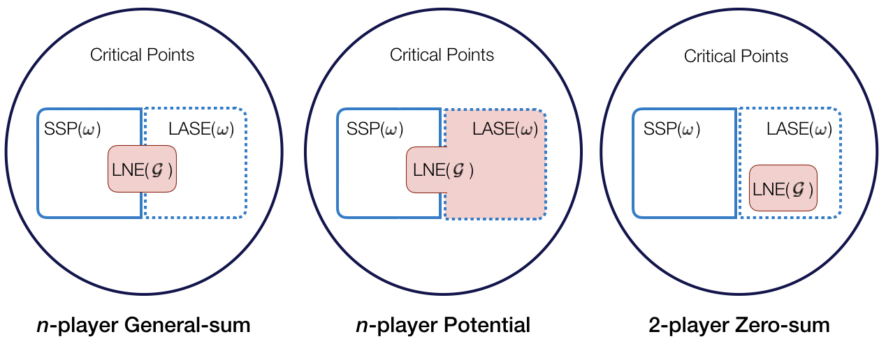
Figure 1: Links between the equilibria of generic continuous games $\mathcal{G}$ and their properties under the gradient dynamics $\dot{x}=-\omega(x)$.

3.1 General-sum games

We first analyze the properties of local Nash equilibria under the joint gradient dynamics in $n$-player general-sum games.

Proposition 5

A non-degenerate differential Nash equilibrium is either a locally asymptotically stable equilibrium or a strict saddle point of $\dot{x}=-\omega(x)$—i.e., ${\tt{NDDNE}}(\mathcal{G})\subset{\tt{SSP}}(\omega)\cup{\tt{LASE}}(\omega)$.

Locally asymptotically stable differential Nash equilibria satisfy the notion of variational stability introduced in Mertikopoulos and Zhou (2019). In fact, a simple analysis shows that the definitions of variationally stable equilibria and locally asymptotically stable differential Nash equilibria Ratliff et al. (2013) are equivalent in the games we consider—i.e., games where each players’ cost is at least twice continuously differentiable. We remark that, from the definition of asymptotic stability, the gradient dynamics have a $O(1/t)$ convergence rate in the neighborhood of such equilibria.

An important point to make is that not every locally asymptotically stable equilibrium of $\dot{x}=-\omega(x)$ is a non-degenerate differential Nash equilibrium. Indeed, the following proposition provides an entire class of games whose corresponding gradient dynamics admit locally asymptotically stable equilibria that are not local Nash equilibria.

Proposition 6

In the class of general-sum continuous games, there exists a continuum of games containing games $\mathcal{G}$ such that ${\tt{LASE}}(\omega)\not\subset{\tt{NDDNE}}(\mathcal{G})$, and moreover, ${\tt{LASE}}(\omega)\not\subset{\tt{LNE}}(\mathcal{G})$.

Proof  Consider a two player game $\mathcal{G}=(f_{1},f_{2})$ on $\mathbb{R}^{2}$ where

$$f_{1}(x_{1},x_{2})=\frac{a}{2}x^{2}_{1}+bx_{1}x_{2},\ \ \text{and}\ \ f_{2}(x_{1},x_{2})=\frac{d}{2}x^{2}_{2}+cx_{1}x_{2}$$

for constants $a,b,c,d\in\mathbb{R}$. The Jacobian of $\omega$ is given by

$$D\omega(x_{1},x_{2})=\begin{bmatrix}a&b\\ c&d\end{bmatrix},\ \ \forall(x_{1},x_{2})\in\mathbb{R}^{2}.$$ (3)

If $a>0$ and $d<0$, then the unique stationary point $x=(0,0)$ is neither a differential Nash nor a local Nash equilibria since the necessary conditions are violated (i.e., $d<0$). However, if $a>-d$ and $ad>cb$, the eigenvalues of $D\omega$ have positive real parts and $(0,0)$ is asymptotically stable. Further, this clearly holds for a continuum of games. Thus, the set of locally asymptotically stable equilibria that are not Nash equilibria may be arbitrarily large.  

The, preceding proposition shows that there exists attracting critical points of the gradient dynamics in general-sum continuous games that are not Nash equilibria and may not be even relevant to the game. Thus, this provides a negative answer to Q2 (whether all attracting equilibria in general-games are game-relevant for the learning dynamics).

Remark 7

We note that, by definition, the non-Nash locally asymptotically stable equilibria (or non-Nash equilibria) do not satisfy the second-order conditions for Nash equilibria. Thus, at these joint strategies, at least one player – and maybe all of them – has a direction in which they would unilaterally deviate if they were not using gradient descent. As such, we view convergence to these points to be undesirable.

3.2 Zero-sum games

Let us now restrict our attention to two-player zero-sum games, which often arise when training GANs, in adversarial learning, and in MARL Goodfellow et al. (2014); Omidshafiei et al. (2017); Chivukula and Liu (2017). In such games, one player can be seen as minimizing $f$ with respect to their decision variable and the other as minimizing $-f$ with respect to theirs. The following proposition shows that all differential Nash equilibria in two-player zero-sum games are locally asymptotically stable equilibria under the flow of $\dot{x}=-\omega(x)$.

Proposition 8

For an arbitrary two-player zero-sum game, $(f,-f)$ on $\mathbb{R}^{m}$, if $x$ is a differential Nash equilibrium, then $x$ is both a non-degenerate differential Nash equilibrium and a locally asymptotically stable equilibrium of $\dot{x}=-\omega(x)$—that is, ${\tt{DNE}}(\mathcal{G})\equiv{\tt{NDDNE}}(\mathcal{G})\subset{\tt{LASE}}(\omega)$.

This result guarantees that the differential Nash equilibria of zero-sum games are isolated and exponentially attracting under the flow of $\dot{x}=-\omega(x)$. This in turn guarantees that simultaneous gradient-play has a local linear rate of convergence to all local Nash equilibria in all zero-sum continuous games. Thus, the answer to Q1 is the context of zero-sum games is “yes”, since all Nash equilibria are attracting for the gradient dynamics.

The converse of the preceding proposition, however, is not true. Not every locally asymptotically stable equilibrium in two-player zero-sum games are non-degenerate differential Nash equilibria. Indeed, there may be many locally asymptotically stable equilibria in a zero-sum game that are not local Nash equilibria. The following proposition highlights this fact.

Proposition 9

In the class of zero-sum continuous games, there exists a continuum of games such that for each game $\mathcal{G}$, ${\tt{LASE}}(\omega)\not\subset{\tt{DNE}}(\mathcal{G})\subset{\tt{LNE}}(\mathcal{G})$.

Proof  Consider the two-player zero-sum game $(f,-f)$ on $\mathbb{R}^{2}$ where

$$f(x_{1},x_{2})=\frac{a}{2}x^{2}_{1}+bx_{1}x_{2}+\frac{c}{2}x^{2}_{2};$$

and $a,b,c\in\mathbb{R}$. The Jacobian of $\omega$ is given by

$$D\omega(x_{1},x_{2})=\begin{bmatrix}\ \ a&\ \ b\\ -b&-c\end{bmatrix},\ \ \forall\ (x_{1},x_{2})\in\mathbb{R}^{2}.$$

If $a>c>0$ and $b^{2}>ac$, then $D\omega(x_{1},x_{2})$ has eigenvalues with strictly positive real part, but the unique stationary point is not a differential Nash equilibrium—since $-c<0$—and, in fact, is not even a Nash equilibrium. Indeed,

$$-f(0,0)>-f(0,x_{2})=-\frac{c}{2}x_{2}^{2},\ \ \forall\ x_{2}\neq 0.$$

Thus, there exists a continuum of zero-sum games with a large set of locally asymptotically stable equilibria of the corresponding dynamics $\dot{x}=-\omega(x)$ that are not differential Nash.  

The, preceding proposition again shows that there exists non-Nash equilibria of the gradient dynamics in zero-sum continuous games. Thus, this proposition also provides a negative answer to Q2 in the context of zero-sum games.

3.3 Potential Games

One last set of games with interesting connections between the Nash equilibria and the critical points of the gradient dynamics is the class known as potential games. This particularly nice class of games are ones for which $\omega$ corresponds to a gradient flow under a coordinate transformation—that is, there exists a function $\phi$ (commonly referred to as the potential function) such that for each $i\in\mathcal{I}$, $D_{i}f_{i}\equiv D_{i}\phi$. We remark that due to the equivalence this class of games is sometimes referred to as an exact potential game. Note that a necessary and sufficient condition for $(f_{1},\ldots,f_{n})$ to be a potential game is that $D\omega$ is symmetric Monderer and Shapley (1996)—that is, $D_{ij}f_{j}\equiv D_{ji}f_{i}$. This gives potential games the desirable property that the only locally asymptotically stable equilibria of the gradient dynamics are local Nash equilibria.

Proposition 10

For an arbitrary potential game, $\mathcal{G}=(f_{1},\ldots,f_{n})$ on $\mathbb{R}^{m}$, if $x$ is a locally asymptotically stable equilibrium of $\dot{x}=-\omega(x)$ (i.e., $x\in{\tt{LASE}}(\omega)$), then $x$ is a non-degenerate differential Nash equilibrium (i.e., $x\in{\tt{NDDNE}}(\mathcal{G})$).

The full proof of Proposition 10 is supplied in Appendix A. The preceding proposition rules out non-Nash locally asymptotically stable equilibria of the gradient dynamics in potential games, and implies that every local minimum of a potential game must be a local Nash equilibrium. Thus, in potential games, unlike in general-sum and zero-sum games, the answer to Q2 is positive. However, the following proposition shows that the existence of a potential function is not enough to rule out local Nash equilibria that are saddle points of the dynamics.

Proposition 11

In the class of continuous games, there exist a continuum of potential games containing games $\mathcal{G}$ that admit Nash equilibria that are saddle points of the dynamics $\dot{x}=-\omega(x)$—i.e., $\exists\ \mathcal{G}$ such that for some $x\in{\tt{LNE}}(\mathcal{G})$, $x\in{\tt{SSP}}(\omega)$.

Proof  Consider the game $(f,f)$ on $X=\mathbb{R}^{2}$ described by

$$f(x_{1},x_{2})=\frac{a}{2}x_{1}^{2}+bx_{1}x_{2}+\frac{c}{2}x_{2}^{2}$$

where $a,b,d\in\mathbb{R}$. The Jacobian of $\omega$ is given by

$$D\omega(x_{1},x_{2})=\begin{bmatrix}a&b\\ b&c\end{bmatrix},\ \ \forall\ (x_{1},x_{2})\in\mathbb{R}^{2}.$$

If $a,c>0$, then $x=(0,0)$ is a local Nash equilibrium. However, if $ac<b^{2}$, $D\omega(x)$ has one positive and one negative eigenvalue and $(0,0)$ is a saddle point of the gradient dynamics. Thus, there exists a continuum of potential games where a large set of differential Nash equilibria are strict saddle points of $\dot{x}=-\omega(x)$.  

Proposition 11 demonstrates a surprising fact about potential games. Even though all minimizers of the potential function must be local Nash equilibria, not all local Nash equilibria are minimizers of the potential function.

3.4 Main Takeaways

The main takeaways of this section are summarized in Figure 1. We note that for zero-sum games, Proposition 9 shows that ${\tt{LNE}}(\mathcal{G})\subset{\tt{LASE}}(\omega)$. Since the inclusion is strict, the answer to Q2 in such games is “no”. For general-sum games, Proposition 6 allows us to to conclude that there do exist attracting, non-Nash equilibria. Thus, the answer to Q2 is also “no”. In potential games, since ${\tt{LASE}}(\omega)\subset{\tt{LNE}}(\mathcal{G})$ the answer is “yes”.

In the following sections, we provide answers to Q1 by showing that all local Nash equilibria in ${\tt{LNE}}(\mathcal{G})\cap{\tt{SSP}}(\omega)$ are avoided almost surely by gradient-based algorithms in both the deterministic and stochastic settings. In particular, since ${\tt{LNE}}(\mathcal{G})\cap{\tt{SSP}}(\omega)\neq\emptyset$ in potential and general-sum games, one cannot give a positive answer to Q1 in either of these classes of games.

4 Convergence of Gradient-Based Learning

In this section, we provide convergence and non-convergence results for gradient-based algorithms. We also include a high-level overview of well-known algorithms that fit into the class of learning algorithms we consider; more detail can be found in Appendix C.

4.1 Deterministic Setting

We first address convergence to equilibria in the deterministic setting in which agents have oracle access to their gradients at each time step. This includes the case where agents know their own cost functions $f_{i}$ and observe their own actions as well as their competitors’ actions—and hence, can compute the gradient of their cost with respect to their own choice variable.

Since we have assumed that each agent $i\in\mathcal{I}$ has their own learning rate (i.e. step sizes $\gamma_{i}$), the joint dynamics of all the players are given by

$$x_{t+1}=g(x_{t})$$ (4)

where $g:x\mapsto x-\gamma\odot\omega(x)$ with $\gamma=(\gamma_{i})_{i\in\mathcal{I}}$ and $\gamma>0$ element-wise. By a slight abuse of notation, $\gamma\odot\omega(x_{t})$ is defined to be element-wise multiplication of $\gamma$ and $\omega(\cdot)$ where $\gamma_{1}$ is multiplied by the first $m_{1}$ components of $\omega(\cdot)$, $\gamma_{2}$ is multiplied by the next $m_{2}$ components, and so on.

We remark that this update rule immediately distinguishes gradient-based learning in games from gradient descent. By definition, the dynamics of gradient descent in single-agent settings always correspond to gradient flows —i.e $x$ evolves according to an ordinary differential equation of the form $\dot{x}=-\nabla\phi(x)$ for some function $\phi:\mathbb{R}^{d}\rightarrow\mathbb{R}$. Outside of the class of exact potential games we defined in Section 3, the dynamics of players’ actions in games are not afforded this luxury—indeed, $D\omega$ is not in general symmetric (which is a necessary condition for a gradient flow). This makes the potential limiting behaviors of $\dot{x}=-\omega(x)$ highly non-trivial to characterize in general-sum games.

The structure present in a gradient-flow implies strong properties on the limiting behaviors of $x$. In particular, it precludes the existence of limit cycles or periodic orbits (limiting behaviors of dynamical systems where the state of system cycles infinitely through a set of states with a finite period) and chaos (an attribute of nonlinear dynamical systems where the system’s behavior can vary extremely due to slight changes in initial position) Sastry (1999). We note that both of these behaviors can occur in the dynamics of gradient-based learning algorithms in games.

Despite the wide breadth of behaviors that gradient dynamics can exhibit in competitive settings, we are still make statements about convergence (and non-convergence) to certain types of equilibria. To do so, we first make the following standard assumptions on the smoothness of the cost functions $f_{i}$ and the magnitude of the agents’ learning rates $\gamma_{i}$.

Assumption 1

For each $i\in\mathcal{I}$, $f_{i}\in C^{s}({X},\mathbb{R})$ with $s\geq 2$, $\sup_{x\in X}\|D\omega(x)\|_{2}\leq L<\infty$, and $0<\gamma_{i}<1/L$ where $\|\cdot\|_{2}$ is the induced $2$-norm.

Given these assumptions, the following result rules out converging to strict saddle points.

Theorem 12

Let $f_{i}:{X}\rightarrow\mathbb{R}$ and $\gamma$ satisfy Assumption 1. Suppose that ${X}=X_{1}\times\cdots\times X_{n}\subseteq\mathbb{R}^{m}$ is open and convex. If $g({X})\subset{X}$, the set of initial conditions $x\in{X}$ from which competitive gradient-based learning converges to strict saddle points is of measure zero.

We remark that the above theorem holds for $X=X_{1}\times\cdots\times X_{n}=\mathbb{R}^{m}$ in particular, since $g(X)\subset X$ holds trivially in this case. It is also important to note that, as we point out in Section 3, local Nash equilibria can be strict saddle points. Thus, all local Nash equilibria that are strict saddle points for $\dot{x}=-\omega(x)$ are avoided almost surely by gradient-play even with oracle gradient access and random initializations. This holds even when players randomly initialize uniformly in an arbitrarily small ball around such Nash equilibria. In Section 5, we show that many linear quadratic dynamic games have a strict saddle point as their global Nash equilibrium. For brevity, we provide the proof of Theorem 12 in Appendix A, and provide a proof sketch below.

Proof [Proof sketch of Theorem 12] The core of the proof is the celebrated stable manifold theorem from dynamical systems theory, presented in Theorem 16. We construct the set of initial positions from which gradient-play will converge to strict saddle points and then use the stable manifold theorem to show that the set must have measure zero in the players’ joint strategy space. Therefore, with a random initialization players will never evolve solely on the stable manifold of strict saddles and they will consequently diverge from such equilibria.

To be able to invoke the stable manifold theorem, we first show that the mapping $g:\mathbb{R}^{m}\rightarrow\mathbb{R}^{m}$ is a diffeomorphism, which is non-trivial due to the fact that we have allowed each agent to have their own learning rate $\gamma_{i}$ and $D\omega$ is not symmetric. We then iteratively construct the set of initializations that will converge to strict saddle points under the game dynamics. By the stable manifold theorem, and the fact that $g$ is a diffeomorphism, the stable manifold of a strict saddle point must be measure zero. Then, by induction we show that the set of all initial points that converge to a strict saddle point must also be measure zero.  

In potential games we can strengthen the above non-convergence result and give convergence guarantees.

Corollary 13

Consider a potential game $(f_{1},\ldots,f_{n})$ on open, convex $X=X_{1}\times\cdots\times X_{n}\subseteq\mathbb{R}^{m}$ and where each $f_{i}\in C^{s}(X,\mathbb{R})$ for $s\geq 3$. Let $\nu$ be a prior measure with support $X$ which is absolutely continuous with respect to the Lebesgue measure and assume $\lim_{t\rightarrow\infty}g^{t}(x)$ exists. Then, under Assumption 1, competitive gradient-based learning converges to non-degenerate differential Nash equilibria almost surely. Moreover, the non-degenerate differential Nash to which it converges is generically a local Nash equilibrium.

Corollary 13 guarantees that in potential games, gradient-play will converge to a differential Nash equilibrium. Combining this with Theorem 4.1 guarantees that the differential Nash equilibrium it converges to is a local minimizer of the potential function. A simple implication of this result is that gradient-based learning in potential games cannot exhibit limit cycles or chaos.

Of note is the fact that the agents do not need to be performing gradient-based learning on $\phi$ to converge to Nash almost surely. That is, they do not need to know the function $\phi$; they simply need to follow the derivative of their own cost with respect to their own choice variable, and they are guaranteed to converge to a local Nash equilibrium that is a local minimizer of the potential function.

We note that convergence to Nash equilibria is a known characteristic of gradient-play in potential games. However, our analysis also highlights that gradient-play will avoid a subset of the Nash equilibria of the game. This is surprising given the particularly strong structural properties of such games. The proof for Corollary 13 is provided in Appendix A and follows from Proposition 10, Theorem 12, and the fact that $D\omega$ is symmetric in potential games.

4.1.1 Implications and Interpretation of Convergence Analysis

Both Theorem 12 and Corollary 13 show that gradient-play in multi-agent settings avoids strict saddles almost surely even in the deterministic setting. Combined with the analysis in Section 3 which shows that (local) Nash equilibria can be strict saddles of the dynamics for general-sum games, this implies that a subset of the Nash equilibria are almost surely avoided by individual gradient-play, a potentially undesirable outcome in view of Q1 (whether all Nash equilibria are attracting for the learning dynamics). In Section 5, we show that the global Nash equilibrium is a saddle point of the gradient dynamics in a large number of randomly sampled LQ dynamic games. This suggests that policy gradient algorithms may fail to converge in such games, which is highly undesired. This is in stark contrast to the single agent setting where policy gradient has been shown to converge to the unique solution of LQR problems Fazel et al. (2018).

In Section 3, we also showed that local Nash equilibria of potential games can be strict saddles points of the potential function. Non-convergence to such points in potential games is not necessarily a bad result since this in turn implies convergence to a local minimizer of the potential function (as shown in Lee et al. (2016); Panageas and Piliouras (2016)) which are guaranteed to be local Nash equilibria of the game. However, these results do imply that one cannot answer “yes” to Q1 in potential games since some of the Nash equilibria are not attracting under gradient-play.

In zero-sum games, where local Nash equilibria cannot be strict saddle points of the gradient dynamics, our result suggests that eventually gradient-based learning algorithms will escape saddle points of the dynamics.

The almost sure avoidance of all equilibria that are saddle points of the dynamics further implies that if (3) converges to a critical point $x$, then $x\in{\tt{LASE}}(\omega)$—i.e., $x$ is locally asymptotically stable for $\dot{x}=-\omega(x)$. This may not be a desired property however, since we showed in Section 3 that zero-sum and general-sum games both admit non-Nash LASE.

Since gradient-play in games generally does not result in a gradient flow, other types of limiting behaviors such as limit cycles can occur in gradient-based learning dynamics. Theorem 12 says nothing about convergence to other limiting behaviors. In the following sections we prove that the results described in this section extend to the stochastic gradient setting. We also formally define periodic orbits in the context of dynamical systems and state stronger results on avoidance of some more complex limiting behaviors like linearly unstable limit cycles.

4.2 Stochastic Setting

We now analyze the stochastic case in which agents are assumed to have an unbiased estimator for their gradient. The results in this section allow us to extend the results from the deterministic setting to a setting where each agent builds an estimate of the gradient of their loss at the current set of strategies from potentially noisy observations of the environment. Thus, we are able to analyze the limiting behavior of a class of commonly used machine learning algorithms for competitive, multi-agent settings. In particular, we show that agents will almost surely not converge to strict saddle points. In Appendix B.1, we show that the gradient dynamics will actually avoid more general limiting behaviors called linearly unstable cycles which we define formally.

To perform our analysis, we make use of tools and ideas from the literature on stochastic approximations (see e.g Borkar (2008)). We note that the convergence of stochastic gradient schemes in the single-agent setting has been extensively studied Robbin (1971); Pemantle (1990); Bottou (2010); Mertikopoulos and Staudigl (2018). We extend this analysis to the behavior of stochastic gradient algorithms in games.

We assume that each agent updates their strategy using the update rule

$$x_{i,t+1}=x_{i,t}-\gamma_{i,t}(D_{i}f_{i}(x_{i,t},x_{-i,t})+w_{i,t+1})$$ (5)

for some zero-mean, finite-variance stochastic process $\{w_{i,t}\}$. Before presenting the results for the stochastic case, let us comment on the different learning algorithms that fit into this framework.

4.2.1 Examples of Stochastic Gradient-Based Learning

Class	Gradient Learning Rule
Gradient-Play	$x_{i}^{+}=x_{i}-\gamma_{i}D_{i}f_{i}(x_{i},x_{-i})$
GANs	$\theta^{+}\ =\theta-\gamma\mathbb{E}[D_{\theta}L(\theta,w)]\$
	$w^{+}=w+\gamma\mathbb{E}[D_{w}L(\theta,w)]$
MA Policy Gradient	$x_{i}^{+}=x_{i}-\gamma_{i}\mathbb{E}[{D_{i}J_{i}}(x_{i},x_{-i})]$
Individual Q-learning	$q_{i}^{+}(u_{i})=q_{i}(u_{i})+\gamma_{i}(r_{i}(u_{i},\pi_{-i}(q_{i},q_{-i}))-q_{i}(u_{i}))$
MA Gradient Bandits	$x_{i,\ell}^{+}=x_{i,\ell}+\gamma_{i}\mathbb{E}[\beta_{i}R_{i}(u_{i},u_{-i})|u_{i}=\ell]$, $\ell=1,\ldots,m_{i}$
MA Experts	$x_{i,\ell}^{+}=x_{i,\ell}+\gamma_{i}\mathbb{E}[R_{i}(u_{i},u_{-i})|u_{i}=\ell]$, $\ell=1,\ldots,m_{i}$

Table 1: Example problem classes that fit into competitive gradient-based learning rules. Details on the derivation of these update rules as gradient-based learning schemes is provided in Appendix C.

The stochastic gradient-based learning setting we study is general enough to include a variety of commonly used multi-agent learning algorithms. The classes of algorithms we include is hardly an exhaustive list, and indeed many extensions and altogether different algorithms exist that can be considered members of this class. In Table 1, we provide the gradient-based update rule for six different example classes of learning problems: (i) gradient-play in non-cooperative continuous games, (ii) GANs, (iii) multi-agent policy gradient, (iv) individual Q-learning, (v) multi-agent gradient bandits, and (vi) multi-agent experts. We provide a detailed analysis of these different algorithms including the derivation of the gradient-based update rules along with some interesting numerical examples in Appendix C. In each of these cases, one can view an agent employing the given algorithm as building an unbiased estimate of their gradient from their observation of the environment.

For example, in multi-agent policy gradient (see, e.g., (Sutton and Barto, 2017, Chapter 13)), agents’ costs are defined as functions of a parameter vector $x_{i}$ that parameterize their policies $\pi_{i}(x_{i})$. The parameters $x_{i}$ are agent $i$’s choice variable. By following the gradient of their loss function, they aim to tune the parameters in order to converge to an optimal policy $\pi_{i}$. Perhaps surprisingly, it is not necessary for agent $i$ to have access to $\pi_{{-i}}(x_{-i})$ or even $x_{-i}$ in order for them to construct an unbiased estimate of the gradient of their loss with respect to their own choice variable $x_{i}$ as long as they observe the sequence of actions, say $u_{-i,t}$, of all other agents generated. These actions are implicitly determined by the other agents’ policies $\pi_{-i}(x_{-i})(\cdot)$. Hence, in this case if agent $i$ observes $\{(r_{j,t},u_{j,t},s_{j,t})$, $\forall\ j\in\mathcal{I}\}$ where $(r_{j},u_{j},s_{j})$ are the reward, action, and state of agent $j$, then this is enough to construct an unbiased estimate of their gradient. We provide further details on multi-agent policy gradient in Appendix C.

4.2.2 Stochastic Gradient Results

Returning to the analysis of (5), we make the following standard assumptions on the noise processes Robbin (1971); Robbins and Siegmund (1985).

Assumption 2

The stochastic process $\{w_{i,t+1}\}$ satisfies the assumptions $\mathbb{E}[w_{i,t+1}|\ \mathcal{F}_{i}^{t}]=0$, $t\geq 0$ and $\mathbb{E}[\|w_{i,t+1}\|^{2}|\ \mathcal{F}_{i}^{t}]\leq\sigma^{2}<\infty$ a.s., for $t\geq 0$, where $\mathcal{F}_{i,t}$ is an increasing family of $\sigma_{i}$-fields—i.e. filtration, or history generated by the sequence of random variables—given by $\mathcal{F}_{i,t}=\sigma_{i}(x_{i,k},w_{i,k},k\leq t),\ t\geq 0$.

We also make new assumptions on the players’ step-sizes. These are standard assumptions in the stochastic approximation literature and are needed to ensure that the noise processes are asymptotically controlled.

Assumption 3

For each $i\in\mathcal{I}$, $f_{i}\in C^{s}(X,\mathbb{R})$ with $s\geq 2$, $D_{i}f_{i}$ is $L_{i}$–Lipschitz with $0<L_{i}<\infty$, the step-sizes satisfy $\gamma_{i,t}\equiv\gamma_{t}$ for all $i\in\mathcal{I}$ and $\sum_{t}\gamma_{t}=\infty$ and $\sum_{t}(\gamma_{t})^{2}<\infty$, and $\sup_{t}\|x_{t}\|<\infty$ a.s.

Let $(a)^{+}=\max\{a,0\}$ and $a\cdot b$ denotes the inner product. The following theorem extends the results of Theorem 12 to the stochastic gradient dynamics in games.

Theorem 14

Consider a game $(f_{1},\ldots,f_{n})$ on $X=X_{1}\times\cdots\times X_{n}=\mathbb{R}^{m}$. Suppose each agent $i\in\mathcal{I}$ adopts a stochastic gradient algorithm that satisfies Assumptions 2 and 3. Further, suppose that for each $i\in\mathcal{I}$, there exists a constant $b_{i}>0$ such that $\mathbb{E}[(w_{i,t}\cdot v)^{+}|\mathcal{F}_{i,t}]\geq b_{i}$ for every unit vector $v\in\mathbb{R}^{m_{i}}$. Then, competitive stochastic gradient-based learning converges to strict saddle points of the game on a set of measure zero.

The proof follows directly from showing that (5) satisfies Theorem 17, provided the assumptions of the theorem hold. The assumption that $\mathbb{E}[(w_{i,t}\cdot v)^{+}|\mathcal{F}_{i,t}]\geq b_{i}$ rules out degenerate cases where the noise forces the stochastic dynamics onto the stable manifold of strict saddle points.

Theorem 14 implies that the dynamics of stochastic gradient-based learning defined in (5), have the same limiting properties as the deterministic dynamics vis-à-vis saddle points. Thus, the implications described in Section 4.1.1 extend to the stochastic gradient setting. In particular, stochastic gradient-based algorithms will avoid a non-negligible subset of the Nash equilibria in general-sum and potential games. Further, in zero-sum and general-sum games, if the players fo converge to a critical point, that point may be a non-Nash equilibrium.

4.2.3 Further Convergence Results for Stochastic Gradient-Play in Games

As we demonstrated in Section 4.1, outside of potential games, the dynamics of gradient-based learning algorithms in games are not gradient flows. As such, the players’ actions can converge to more complex sets than simple equilibria. A particularly prominent class of limiting behaviors for dynamical systems are known as limit cycles (see e.g Sastry (1999)). Limit cycles (or periodic orbits) are sets of states $\mathcal{S}$ such that each state $x\in\mathcal{S}$ is visited at periodic intervals ad infinitum under the dynamics. Thus, if the gradient-based algorithms converge to a limit cycle they will cycle infinitely through the same sequence of actions. Like equilibria, limit cycles can be stable or unstable under the dynamics $\dot{x}=-\omega(x)$, meaning that the dynamics can either converge to or diverge from them depending on their initializations.

We remark that the existence of oscillatory behaviors and limit cycles has been observed in the dynamics of of gradient-based learning in various settings like the training of Generative Adversarial Networks Daskalakis et al. (2017), and multiplicative weights in finite action games Mertikopoulos et al. (2018). We simply emphasize that the existence of such limiting behaviors is due to the fact that the dynamics are no longer gradient flows. This fact also allows for other complex limiting behaviors like chaos to exist in the dynamics of gradient-based learning in games. We also show in Appendix B.1 that gradient-based learning avoids some limit cycles.

In Appendix B.1, we formalize the notion of a limit cycle and its stability in the stochastic setting. Using these concepts, we then provide an analogous theorem to Theorem 14 which states that competitive stochastic gradient-based learning converges to linearly unstable limit cycles—a parallel notion to strict saddle points but pertaining to more general limit sets—on a set of measure zero, provided that analogous assumptions to those in the statement of Theorem 14 hold. Providing such guarantees requires a bit more mathematical formalism, and as such we leave the details of these results to Appendix B.

In pursuit of a more general class of games with desirable convergence properties, in Appendix B.2 we also introduce a generalization of potential games, namely Morse-Smale games, for which the combined gradient dynamics correspond to a Morse-Smale vector field Hirsch (1976); Palis and Smale (1970). In such games players are guaranteed to converge to only (linearly stable) cycles or equilibria. In such games, however, players may still converge to non-Nash equilibria and avoid a subset of the Nash equilibria.

5 Saddle Point LNE in LQ Dynamic Games

In this section, we present empirical results that show that a non-negligible subset of two-player LQ games have local Nash equilibria that are strict saddle points of the gradient dynamics. LQ games serve as good benchmarks for analyzing the limiting behavior of gradient-play in a non-trivial setting since they are known to admit global Nash equilibria that can be found be solving a coupled set of Riccati equations Basar and Olsder (1998). LQ games can also be cast as multi-agent reinforcement learning problems where each agent has a policy that is a linear function of the state and a quadratic reward function. Gradient-play in LQ games can therefore be seen as a form of policy gradient.

The empirical results we now present imply that, even in the relatively straightforward case of linear dynamics, linear feedback policies, and quadratic costs, policy gradient multi-agent reinforcement learning would be unable to find the local Nash equilibrium in a non-negligible subset of problems.

LQ game setup

For simplicity, we consider two-player LQ games in $\mathbb{R}^{2}$. Consider a discrete time dynamical system defined by

$$z(t+1)=Az(t)+B_{1}u_{1}(t)+B_{2}u_{2}(t)$$ (6)

where $z(t)\in\mathbb{R}^{2}$ is the state at time $t$, $u_{1}(t)$ and $u_{2}(t)$ are the control inputs of players $1$ and $2$, respectively, and $A$, $B_{1}$, and $B_{2}$ are the system matrices. We assume that player $i$ searches for a linear feedback policy of the form $u_{i}(t)=-K_{i}z(t)$ that minimizes their loss which is given by

$$\textstyle f_{i}(z_{0},u_{1},u_{2})=\sum_{t=0}^{\infty}z(t)^{T}Q_{i}z(t)+u_{i}(t)^{T}R_{i}u_{i}(t)$$

where $Q_{i}\succ 0$ and $R_{i}\succ 0$ are the cost matrices on the state and input, respectively. We note that the two players are coupled through the dynamics since $z(t)$ is constrained to obey the update equation (6). The vector of player derivatives is given by $\omega(K_{1},K_{2})=(D_{1}f_{1}(K_{1},K_{2}),D_{2}f_{2}(K_{1},K_{2}))$ where

$$D_{i}f_{i}(K_{1},K_{2})\textstyle=(R_{ii}K_{i}+B_{i}^{T}P_{i}(B_{1}K_{1}+B_{2}K_{2})-B_{i}^{T}P_{i}A)\sum_{t=0}^{\infty}z(t)z(t)^{T},\ i\in\{1,2\}.$$

Note that there is a slight abuse of notation here as we are treating $D_{i}f_{i}$ as a matrix and as the vectorization of a matrix. The matrices $P_{1}$ and $P_{2}$ can be found by solving the Riccati equations

$$P_{i} =(A-B_{1}K_{1}-B_{2}K_{2})^{T}P_{i}(A-B_{1}K_{1}-B_{2}K_{2})+K_{i}^{T}R_{i}K_{i}+Q_{i},\ \ i\in\{1,2\},$$

for a given $(K_{1},K_{2})$. As shown in Basar and Olsder (1998), global Nash equilibria of LQ games can be found by solving coupled Ricatti equations. Under the following assumption, this can be done using an analogous method to the method of Lyapunov iterations outlined in Li and Gajic (1995) for continuous time LQ games.

Assumption 4

Either $(A,B_{1},\sqrt{Q_{1}})$ or $(A,B_{2},\sqrt{Q_{2}})$ is stabilizable-detectable.

Further information on the uniqueness of Nash equilibria in LQ games and the method of Lyapunov iterations can be found in Basar and Olsder (1998) and Li and Gajic (1995) respectively.

Generating LQ games with strict saddle point Nash equilibria

Without loss of generality, we assume $(A,B_{1},\sqrt{Q_{1}})$ is stabilizable-detectable. Given that we have a method of finding the global Nash equilibrium of the LQ game, we now present our experimental setup.

We fix $B_{1}$, $B_{2}$, $Q_{1}$, and $R_{1}$ and parametrize $Q_{2}$, and $R_{2}$ by $q$ and $r$ respectively. The shared dynamics matrix $A$ has entries that are sampled from the uniform distribution supported on $(0,1)$. For each value of the parameters $b$, $q$, and $r$, we randomly sample $1000$ different $A$ matrices. Then, for each LQ game defined in terms of each of the sets of parameters, we find the optimal feedback matrices $(K_{1}^{*},K_{2}^{*})$ using the method of Lyapunov iterations, and we numerically approximate $D\omega(K_{1}^{*},K_{2}^{*})$ using auto-differentiation tools and check its eigenvalues.

The exact values of the matrices are defined as follows: $A\in\mathbb{R}^{2\times 2}$ with each of the entries $a_{ij}$ sampled from the uniform distribution on $(0,1)$,

$$B_{1}=\begin{bmatrix}1\\ 1\end{bmatrix},\ B_{2}=\begin{bmatrix}0\\ 1\end{bmatrix},\ Q_{1}=\begin{bmatrix}0.01&0\\ 0&1\end{bmatrix},\ Q_{2}=\begin{bmatrix}1&0\\ 0&q\end{bmatrix},\ R_{1}=0.01,\ R_{2}=r.$$

The results for various combinations of the parameters $q$ and $r$ are shown in Figure 2. For all of the different parameter configurations considered, we found that in anywhere from $0\%-25\%$ of the randomly sampled LQ games, there was a global Nash equilibrium that was a strict saddle point of the gradient dynamics. Of particular interest is the fact that for all values of $q$ and $r$ we tested, at least $5\%$ of the LQ games had a global Nash equilibrium with the strict saddle property. In the worst case, around $25\%$ of the LQ games for the given values of $q$ and $r$ admitted such Nash equilibria.

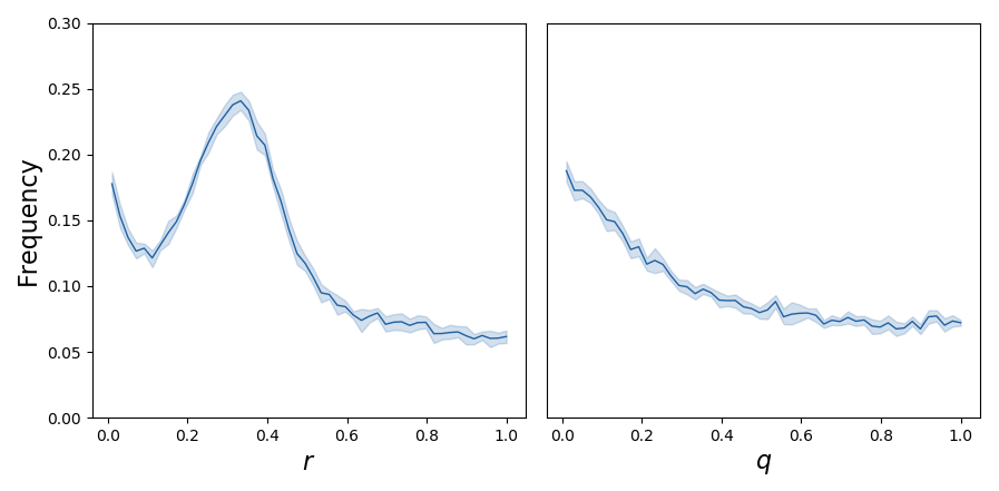
Figure 2: Frequency (out of 1000) of randomly sampled LQ games with global Nash equilibria that are avoided by policy-gradient. The experiment was run 10 times and the average frequency is shown by the solid line. The shaded region demarcates the $95\%$ confidence interval of the experiment. (left) $r$ is varied in $(0,1)$, $q=0.01$. (right) $q$ is varied in $(0,1)$, $r=0.1$.

Remark 15

These empirical observations imply that multi-agent policy gradient, even in the relatively straightforward setting of linear dynamics, linear policies, and quadratic costs, has no guarantees of convergence to the global Nash equilibria in a non-negligible number of games. Further investigation is warranted to validate this fact theoretically. This in turn supports the idea that for more complicated cost functions, policy classes, and dynamics, local Nash equilibria with the strict saddle property are likely to be very common.

6 Discussion and Future Directions

In this paper we provided answers to the following two questions for classes of gradient-based learning algorithms:

Q1.

Are all attractors of the learning algorithms employed by agents equilibria relevant to the underlying game?

Q2.

Are all equilibria relevant to the game also attractors of the learning algorithms agents employ?

We answered these questions in general-sum, zero-sum, and potential games without imposing structure on the game outside regularity conditions on the cost functions by exploiting the observation that gradient-based learning dynamics are not gradient flows. Our analysis, was shown in Section C to apply to a number of commonly used methods in multi-agent learning.

6.1 Links with Prior Work

As we noted, previous work on learning in games in both the game theory literature, and more recently from the machine learning community, has largely focused on Q1, though some recent work has analyzed Q2 in the setting of zero-sum games.

In the seminal work by Rosen Rosen (1965), $n$–player concave or monotone games are shown to either admit a unique Nash equilibrium or a continuum of Nash equilibria, all of which are attracting under gradient-play. The structure present in these games rules out the existence of non-Nash equilibria.

Two-player, finite-action bilinear games have also been extensively studied. In Singh et al. (2000), the authors investigate the convergence of the gradient dynamics in such games. Additionally, the dynamics of other (non gradient-based) algorithms like multiplicative weights have been studied in Hommes and Ochea (2012) among many others. In such settings, the structure guarantees that there exists a unique global Nash equilibrium and no other critical points of the gradient dynamics. As such, non-Nash equilibria, cannot exist.

In the study of learning dynamics in the class of zero-sum games, it has been shown that cycles can be attractors of the dynamics (see, e.g., Mertikopoulos et al. (2018); Wesson and Rand (2016); Hommes and Ochea (2012)). Concurrently with our results, Daskalakis and Panageas (2018) also showed the existence of non-Nash attracting equilibria in this setting.

In more general settings, there has been some analysis of the limiting behavior of gradient-play though the focus has been for the most part, on giving sufficient conditions under which Nash equilibria are attracting under gradient-play. For example,  Ratliff et al. (2013, 2014, 2016), introduced the notion of a differential Nash equilibrium which is characterized by first and second order conditions on the players’ individual cost functions and which we made extensive use of. Following this body of work, Mertikopoulos and Zhou (2019) also investigated the local convergence of gradient-play in continuous games. They showed that if a Nash equilibrium satisfies a property known as variational stability, the equilibrium is attracting under gradient play. In twice continuously differentiable games, this condition coincides exactly with the definition of stable differential Nash equilibria. Though these works analyze a general class of games, the focus of the analysis is solely on the local characterization and computation (via gradient play) of local Nash equilibria. As such, the issues of non-convergence that we show in this paper were not discussed.

6.2 Open Questions

Our results suggest that gradient-play in multi-agent settings has fundamental problems. Depending on the players’ costs, in general games and even potential games, which have a particularly nice structure, a subset of the Nash equilibria will be almost surely avoided by gradient-based learning when the agents randomly initialize their first action. In zero-sum and general-sum games, even if the algorithms do converge, they may have converged to a point that has no game theoretic relevance, namely a non-Nash locally asymptotically stable equilibrium.

Lastly, these results show that limit cycles persist even under a stochastic update scheme. This explains the empirical observations of limit cycles in gradient dynamics presented in  Daskalakis et al. (2017); Leslie and Collins (2005); Hommes and Ochea (2012). It also implies that gradient-based learning in multi-agent reinforcement learning, multi-armed bandits, generative adversarial networks, and online optimization all admit limit cycles under certain loss functions. Our empirical results show that these problems are not merely of theoretical interest, but also have great relevance in practice.

Which classes of games have all Nash being attracting for gradient-play and which classes preclude the existence of non-Nash equilibria is an open and particularly interesting question. Further, the question of whether gradient-based algorithms can be constructed for which only game-theoretically relevant equilibria are attracting is of particular importance as gradient-based learning is increasingly implemented in game theoretic settings. Indeed, more generally, as learning algorithms are increasingly deployed in markets and other competitive environments understanding and dealing with such theoretical issues will become increasingly important.

A Proofs of the Main Results

This appendix contains the full proofs of the results in the paper.

A.1 Proofs on Links Between Dynamical Systems and Games

We begin with a proof of Proposition 5 that all differential Nash equilibria are either strict saddle points or asymptotically stable equilibria of the gradient dynamics. This relies mainly on the definitions of strict saddle points, locally asymptotically stable equilibria, and non-degenerate differential Nash equilibria and simple linear algebra.

Proof [Proof of Proposition 5] Suppose that $x\in X$ is a non-degenerate differential Nash equilibrium. We claim that $\mathrm{tr}(D\omega(x))>0$. Since $x$ is a differential Nash equilibrium, $D_{i}^{2}f_{i}(x)\succ 0$ for each $i\in\mathcal{I}$; these are the diagonal blocks of $D\omega(x)$. Further $D_{i}^{2}f_{i}(x)\succ 0$ implies that $\mathrm{tr}(D_{i}^{2}f_{i}(x))>0$. Since $\mathrm{tr}(D\omega)=\sum_{i=1}^{n}\mathrm{tr}(D_{i}^{2}f_{i}(x))$, $\mathrm{tr}(D\omega(x))>0$. Thus, it is not possible for all the eigenvalues to have negative real part. Since $x$ is non-degenerate, $\det(D\omega(x))\neq 0$ so that none of the eigenvalues can have zero real part. Hence, at least one eigenvalue has strictly positive real part.

To complete the proof, we show that the conditions for non-degenerate differential Nash equilibrium are not sufficient to guarantee that $x$ is locally asymptotically stable for the gradient dynamics—that is, not all eigenvalues of $D\omega(x)$ have strictly positive real part. We do this by constructing a class of games with the strict saddle point property. Consider a class of two player games $\mathcal{G}=(f_{1},f_{2})$ on $\mathbb{R}\times\mathbb{R}$ defined as follows:

$$(f_{1}(x_{1},x_{2}),f_{2}(x_{1},x_{2}))=\Big{(}\frac{a}{2}x_{1}^{2}+bx_{1}x_{2},\frac{d}{2}x_{2}^{2}+cx_{1}x_{2}\Big{)}.$$

In this game, the Jacobian of the gradient dynamics is given by

$$D\omega(x)=\begin{bmatrix}a&b\\ c&d\end{bmatrix}$$ (7)

with $a,b,c,d\in\mathbb{R}$. If $x$ is a non-degenerate differential Nash equilibria, $a,d>0$ and $\det(D\omega(x))\neq 0$ which implies that $ad\neq cb$. Choosing $c,d$ such that $ad<cb$ will guarantee that one of the eigenvalues of $D\omega(x)$ is negative and the other is positive, making $x$ a strict saddle point. This shows that non-degenerate differential Nash equilibria can be strict saddle points of the combined gradient dynamics.

Hence, for any game $(f_{1},\ldots,f_{n})$, a non-degenerate differential Nash equilibrium is either a locally asymptotically stable equilibrium or a strict saddle point, but it not strictly unstable or strictly marginally stable (i.e. having eigenvalues all on the imaginary axis).  

The proof of Proposition 8, which claims that all differential Nash equilibria in zero-sum games are locally asymptotically stable, again just relies on basic linear algebra and the definition of a differential Nash equilibrium.

Proof [Proof of Proposition 8] Consider a two player game $(f,-f)$ on $X_{1}\times X_{2}=\mathbb{R}^{m}$ with $X_{i}=\mathbb{R}^{m_{i}}$. For such a game,

$$D\omega(x)=\begin{bmatrix}\ \ D_{1}^{2}f(x)&\ \ D_{21}f(x)\\ -D_{12}f(x)&-D_{2}^{2}f(x)\end{bmatrix}.$$

Note that $D_{21}f(x)=(D_{12}f(x))^{T}$. Suppose that $x=(x_{1},x_{2})$ is a differential Nash equilibrium and let $v=[v_{1},v_{2}]\in\mathbb{R}^{m}$ with $v_{1}\in\mathbb{R}^{m_{1}}$ and $v_{2}\in\mathbb{R}^{m_{2}}$. Then, $v^{T}D\omega(x)v=v_{1}^{T}D_{1}^{2}f(x)v_{1}-v_{2}^{T}D_{2}^{2}f(x)v_{2}>0$ since $D_{1}^{2}f(x)\succ 0$ and $-D_{2}^{2}f(x)\succ 0$ for $x$, a differential Nash equilibrium. Since $v$ is arbitrary, this implies that $D\omega(x)$ is positive definite and hence, clearly non-degenerate. Thus, for two-player zero-sum games, all differential Nash equilibria are both non-degenerate differential Nash equilibria and locally asymptotically stable equilibria of $\dot{x}=-\omega(x)$  

The proof that all locally asymptotically stable equilibria in potential games are differential Nash equilibria relies on the symmetry of $D\omega$ in potential games.

Proof [Proof of Proposition 10] The proof follows from the definition of a potential game. Since $(f_{1},$ $\ldots,f_{n})$ is a potential game, it admits a potential function $\phi$ such that $D_{i}f_{i}(x)=D_{i}\phi(x)$ for all $x$. This, in turn, implies that at a locally asymptotically stable equilibrium of $\dot{x}=-\omega(x)$, $D\omega(x)=D^{2}\phi(x)$, where $D^{2}\phi$ is the Hessian matrix of the function $\phi$. Further $D^{2}\phi(x)$ must have strictly positive eigenvalues for $x$ to be a locally asymptotically stable equilibrium of $\dot{x}=-\omega(x)$. Since the Hessian matrix of a function must be symmetric, $D^{2}\phi(x)$, must be positive definite, which through Sylvester’s criterion ensures that each of the diagonal blocks of $D^{2}\phi(x)$ is positive definite. Thus, we have that the existence of a potential function guarantees that the only locally asymptotically stable equilibria of $\dot{x}=-\omega(x)$, are differential Nash equilibria.  

A.2 Proofs for Deterministic Setting

We now present the proof of Theorem 12 and its corollaries. The proof of relies on the celebrated stable manifold theorem (Shub, 1978, Theorem III.7), Smale (1967). Given a map $\phi$, we use the notation $\phi^{t}=\phi\circ\cdots\circ\phi$ to denote the $t$–times composition of $\phi$.

Theorem 16 (Center and Stable Manifolds (Shub, 1978, Theorem III.7), Smale (1967))

Let $x_{0}$ be a fixed point for the $C^{r}$ local diffeomorphism $f:U\rightarrow\mathbb{R}^{d}$ where $U\subset\mathbb{R}^{d}$ is an open neighborhood of $x_{0}$ in $\mathbb{R}^{d}$ and $r\geq 1$. Let $E^{s}\oplus E^{c}\oplus E^{u}$ be the invariant splitting of $\mathbb{R}^{d}$ into generalized eigenspaces of $D\phi(x_{0})$ corresponding to eigenvalues of absolute value less than one, equal to one, and greater than one. To the $D\phi(x_{0})$ invariant subspace $E^{s}\oplus E^{c}$ there is an associated local $\phi$–invariant $C^{r}$ embedded disc $W_{\text{loc}}^{cs}$ called the local stable center manifold of dimension $\dim(E^{s}\oplus E^{c})$ and ball $B$ around $x_{0}$ such that $\phi(W_{\text{loc}}^{cs})\cap B\subset W_{\text{loc}}^{cs}$, and if $\phi^{t}(x)\in B$ for all $t\geq 0$, then $x\in W_{\text{loc}}^{sc}$.

Some parts of the proof follow similar arguments to the proofs of results in Lee et al. (2016); Panageas and Piliouras (2016) which apply to (single-agent) gradient-based optimization. Due to the different learning rates employed by the agents and the introduction of the differential game form $\omega$, the proof differs.

Proof [Proof of Theorem 12] The proof is composed of two parts: (a) the map $g$ is a diffeomorphism, and (b) application of the stable manifold theorem to conclude that the set of initial conditions is measure zero.

(a) $g$ is diffeomorphism

We claim the mapping $g:\mathbb{R}^{m}\rightarrow\mathbb{R}^{m}$ is a diffeomorphism. If we can show that $g$ is invertible and a local diffeomorphism, then the claim follows. Consider $x\neq y$ and suppose $g(y)=g(x)$ so that $y-x=\gamma\cdot(\omega(y)-\omega(x))$. The assumption $\sup_{x\in\mathbb{R}^{m}}\|D\omega(x)\|_{2}\leq L<\infty$ implies that $\omega$ satisfies the Lipschitz condition on $\mathbb{R}^{m}$. Hence, $\|\omega(y)-\omega(x)\|_{2}\leq L\|y-x\|_{2}$. Let $\Gamma=\operatorname{diag}({\Gamma}_{1},\ldots,{\Gamma}_{n})$ where ${\Gamma}_{i}=\operatorname{diag}((\gamma_{i})_{j=1}^{m_{i}})$—that is, ${\Gamma}_{i}$ is an $m_{i}\times m_{i}$ diagonal matrix with $\gamma_{i}$ repeated on the diagonal $m_{i}$ times. Then, $\|x-y\|_{2}\leq L\|\Gamma\|_{2}\|y-x\|_{2}<\|y-x\|_{2}$ since $\|\Gamma\|_{2}=\max_{i}|\gamma_{i}|<1/L$.

Now, observe that $Dg=I-\Gamma D\omega(x)$. If $Dg$ is invertible, then the implicit function theorem (Lee, 2012, Theorem C.40) implies that $g$ is a local diffeomorphism. Hence, it suffices to show that $\Gamma D\omega(x)$ does not have an eigenvalue of $1$. Indeed, letting $\rho(A)$ be the spectral radius of a matrix $A$, we know in general that $\rho(A)\leq\|A\|$ for any square matrix $A$ and induced operator norm $\|\cdot\|$ so that $\rho(\Gamma D\omega(x))\leq\|\Gamma D\omega(x)\|_{2}\leq\|\Gamma\|_{2}\sup_{x\in\mathbb{R}^{m}}\|D\omega(x)\|_{2}<\max_{i}|\gamma_{i}|L<1$ Of course, the spectral radius is the maximum absolute value of the eigenvalues, so that the above implies that all eigenvalues of $\Gamma D\omega(x)$ have absolute value less than $1$.

Since $g$ is injective by the preceding argument, its inverse is well-defined and since $g$ is a local diffeomorphism on $\mathbb{R}^{m}$, it follows that $g^{-1}$ is smooth on $\mathbb{R}^{m}$. Thus, $g$ is a diffeomorphism.

(b) Application of the stable manifold theorem

Consider all critical points to the game—i.e. $\mathcal{X}_{c}=\{x\in{X}|\ \omega(x)=0\}$. For each $p\in\mathcal{X}_{c}$, let $B_{p}$ be the open ball derived from Theorem 16 and let $\mathcal{B}=\cup_{p}B_{p}$. Since ${X}\subseteq\mathbb{R}^{m}$, Lindelõf’s lemma Kelley (1955)—every open cover has a countable subcover—gives a countable subcover of $\mathcal{B}$. That is, for a countable set of critical points $\{p_{i}\}_{i=1}^{\infty}$ with $p_{i}\in\mathcal{X}_{c}$, we have that $\mathcal{B}=\cup_{i=1}^{\infty}B_{p_{i}}$.

Starting from some point $x_{0}\in X$, if gradient-based learning converges to a strict saddle point, then there exists a $t_{0}$ and index $i$ such that $g^{t}(x_{0})\in B_{p_{i}}$ for all $t\geq t_{0}$. Again, applying Theorem 16 and using that $g(X)\subset X$—which we note is obviously true if $X=\mathbb{R}^{m}$—we get that $g^{t}(x_{0})\in W_{\text{loc}}^{cs}\cap X$.

Using the fact that $g$ is invertible, we can iteratively construct the sequence of sets defined by $W_{1}(p_{i})=g^{-1}(W_{\text{loc}}^{cs}\cap X)$ and $W_{k+1}(p_{i})=g^{-1}(W_{k}(p_{i})\cap X)$. Then we have that $x_{0}\in W_{t}(p_{i})$ for all $t\geq t_{0}$. The set $\mathcal{X}_{0}=\cup_{i=1}^{\infty}\cup_{t=0}^{\infty}W_{t}(p_{i})$ contains all the initial points in $X$ such that gradient-based learning converges to a strict saddle. Since $p_{i}$ is a strict saddle, $I-\Gamma D\omega(p_{i})$ has an eigenvalue greater than $1$. This implies that the co-dimension of $E^{u}$ is strictly less than $m$. (i.e. $\dim(W_{\text{loc}}^{cs})<m$). Hence, $W_{\text{loc}}^{cs}\cap X$ has Lebesgue measure zero in $\mathbb{R}^{m}$.

Using again that $g$ is a diffeomorphism, $g^{-1}\in C^{1}$ so that it is locally Lipschitz and locally Lipschitz maps are null set preserving. Hence, $W_{k}(p_{i})$ has measure zero for all $k$ by induction so that $\mathcal{X}_{0}$ is a measure zero set since it is a countable union of measure zero sets.  

The proof of Corollary 13 follows from the symmetry of $D\omega$ in potential games, and our observations in Section 3.

Proof [Proof of Corollary 13] Since the game admits a potential function $\phi$, there is a transformation of coordinates such that agents following the dynamics $x_{t+1}=x_{t}-\gamma\odot\omega(x_{t})$ converge to the same equilibria as the gradient dynamics $x_{t+1}=x_{t}-\gamma\odot D\phi(x_{t})$. Hence, the analysis of the gradient-based learning scheme reduces to analyzing gradient-based optimization of $\phi$. Moreover, existence of a potential function also implies that $D_{ij}f_{j}\equiv D_{ji}f_{i}$ so that $D\omega$ is symmetric. Indeed, writing $\omega(x)$ as the differential form $\sum_{i=1}^{n}D_{i}f_{i}(x)\mathrm{d}x_{i}$ and noting that $\mathrm{d}\circ\mathrm{d}=0$ for the differential operator $d$, we have that $\mathrm{d}(\omega)=\sum_{i}\mathrm{d}(D_{i}f_{i})\wedge\mathrm{d}x_{i}=\sum_{i,j:j>i}\left(D_{ij}f_{j}-D_{ji}f_{i}\right)\mathrm{d}x_{i}\wedge\mathrm{d}x_{j}=0$ where $\wedge$ is the standard exterior product Lee (2012). Symmetry of $D\omega$ implies that all periodic orbits are equilibria—i.e. the dynamics do not possess any limit cycles. By Theorem 12, the set of initial points that converge to strict saddle points is of measure zero. Since all the stable critical points of the dynamics are equilibria, with the assumption that $\lim_{t\rightarrow\infty}g^{t}(x)$ exists for all $x\in X$, we have that $P_{\nu}\left[\lim_{t\rightarrow\infty}g^{t}(x)=x^{\ast}\right]=1$ where $x^{\ast}$ is a non-degenerate differential Nash equilibrium which is generically a local Nash equilibrium Ratliff et al. (2014).

 

A.3 Classical Results from Dynamical Systems

The remaining results use the following classical result from dynamical systems theory. Consider a general stochastic approximation framework $x_{t+1}=x_{t}+\gamma_{t}(h(x_{t}))+\epsilon_{t}$ for $h:X\rightarrow TX$ with $h\in C^{2}$ and where $X\subset\mathbb{R}^{d}$ and where $TX$ denotes the tangent space.

Theorem 17 (Theorem 1 Pemantle (1990))

Suppose $\gamma_{t}$ is $\mathcal{F}_{t}$–measurable and $\mathbb{E}[w_{t}|\mathcal{F}_{t}]=0$. Let the stochastic process $\{x_{t}\}_{t\geq 0}$ be defined as above for some sequence of random variables $\{\epsilon_{t}\}$ and $\{\gamma_{t}\}$. Let $p\in X$ with $h(p)=0$ and let $W$ be a neighborhood of $p$. Assume that there are constants $\eta\in(1/2,1]$ and $c_{1},c_{2},c_{3},c_{4}>0$ for which the following conditions are satisfied whenever $x_{t}\in W$ and $t$ sufficiently large: (i) $p$ is a linear unstable critical point, (ii) $c_{1}/t^{\eta}\leq\gamma_{t}\leq c_{2}/t^{\eta}$, (iii) $\mathbb{E}[(w_{t}\cdot v)^{+}|\mathcal{F}_{t}]\geq c_{3}/t^{\eta}$ for every unit vector $v\in TX$, and (iv) $\|w_{t}\|_{2}\leq c_{4}/t^{\eta}$. Then $P(x_{t}\rightarrow p)=0$.

B Expanded Results in the Stochastic Setting

In this appendix , we provide extended results in the stochastic setting that require more mathematical formalism than the main body of the paper. In addition, we introduce a new class of games that generalize potential games and have stronger convergence guarantees than the broader class of general-sum continuous games.

B.1 Avoidance of Repelling Sets

To show that stochastic gradient-based learning avoids of more general limiting behaviors than saddle points, we need further assumptions on our underlying space—i.e. we need the underlying decision spaces of each agent—i.e. $X_{i}$ for each $i\in\mathcal{I}$—to be smooth, compact manifolds without boundary. The stochastic process $\{x_{n}\}$ which follows (5) is defined on $X$—that is, $x_{n}\in X$ for all $n\geq 0$. As before, it is natural to compare sample points $\{x_{n}\}$ to solutions of $\dot{x}=-\omega(x)$ where we think of (5) as a noisy approximation. The asymptotic behavior of $\{x_{n}\}$ can indeed be described by the asymptotic behavior of the flow generated by $\omega$.

We also need a formal notion of cycles. A non-stationary periodic orbit of $\omega$ is called a cycle. Let $\xi\subset X$ be a cycle of period $T>0$. Denote by $\Phi_{T}$ the flow corresponding to $\omega$. For any $x\in\xi$, $\mathrm{spec}(D\Phi_{T}(x))=\{1\}\cup C(\xi)$ where $C(\xi)$ is the set of characteristic multipliers. We say $\xi$ is hyperbolic if no element of $C(\xi)$ is on the complex unit circle. Further, if $C(\xi)$ is strictly inside the unit circle, $\xi$ is called linearly stable and, on the other hand, if $C(\xi)$ has at least one element on the outside of the unit circle—that is, $D\Phi_{T}(x)$ for $x\in\xi$ has an eigenvalue with real part strictly greater than $1$—then $\xi$ is called linearly unstable. The latter is the analog of strict saddle points in the context of periodic orbits. We denote by $\{x_{t}\}$ sample paths of the process (5) and $L(\{x_{t}\})$ is the limit set of any sequence $\{x_{t}\}_{t\geq 0}$ which is defined in the usual way as all $p\in X$ such that $\lim_{k\rightarrow\infty}x_{t_{k}}=p$ for some sequence $t_{k}\rightarrow\infty$. It was shown in Benaïm (1996) that under less restrictive assumptions than Assumptions 2 and 3, $L(\{x_{t}\})$ is contained in the chain recurrent set of $\omega$ and $L(\{x_{t}\})$ is a non-empty, compact and connected set invariant under the flow of $\omega$.

Theorem 18

Consider a game $(f_{1},\ldots,f_{n})$ where each $X_{i}$ is a smooth, compact manifold without boundary. Suppose each agent $i\in\mathcal{I}$ adopts a stochastic gradient-based learning algorithm that satisfies Assumptions 2 and 3 and is such that sample points $x_{t}\in X$ for all $t\geq 0$. Further, suppose that for each $i\in\mathcal{I}$, there exist a constant $b_{i}>0$ such that $\mathbb{E}[(w_{i,t}\cdot v)^{+}|\mathcal{F}_{i,t}]\geq b_{i}$ for every unit vector $v\in\mathbb{R}^{m_{i}}$. Then competitive stochastic gradient-based learning converges to linearly unstable cycles on a set of measure zero—i.e. $P(L(x_{t})=\xi)=0$ where $\{x_{t}\}$ is a sample path.

As we noted, periodic orbits are not necessarily excluded from the limiting behavior of gradient-based learning in games. We leave out the proof of Theorem 18 since after some algebraic manipulation, it is a direct application of (Benaïm and Hirsch, 1995, Theorem 2.1) which is stated below.

Theorem 19 (Theorem 2.1 Benaïm and Hirsch (1995))

Let $\xi\subset X$ be a hyperbolic linearly unstable cycle of $h$. Assume the following (i) $h\in C^{2}$; (ii) $c_{1}/t^{\eta}\leq\gamma_{t}\leq c_{2}/t^{\eta}$ with $0<c_{1}\leq c_{2}$ and $0<\eta\leq 1$; and (iii) there exists $b\geq 0$ such that for all unit vectors $v\in\mathbb{R}^{m}$, $\mathbb{E}[(w_{t}\cdot v)^{+}|\mathcal{F}_{t}]\geq b$. Then $P(L(\{x_{t}\})=\xi)=0$.

B.2 Morse-Smale Games

For a class of games admitting gradient-like vector fields we can go beyond non-convergence results and give convergence guarantees. Following Benaïm and Hirsch (1995), we introduce a new class of games, which we call Morse-Smale games, that are a generalization of potential games. Such games represent an important class since the vector field of $\omega$ corresponds to Morse-Smale vector field which is known to be generic in $\mathbb{R}^{2}$ and are otherwise structurally stable Hirsch (1976); Palis and Smale (1970).

Definition 20

A game $(f_{1},\ldots,f_{n})$ with $f_{i}\in C^{r}$ for some $r\geq 3$ and where strategy spaces $X_{i}$ is a smooth, compact manifold without boundary for each $i\in\mathcal{I}$ is a Morse-Smale game if the vector field corresponding to the differential $\omega$ is Morse-Smale—that is, the following hold: (i) all periodic orbits $\xi$ (i.e. equilibria and cycles) are hyperbolic and $W^{s}(\xi)\pitchfork W^{u}(\xi)$ (i.e. the stable and unstable manifolds of $\xi$ intersect transversally), (ii) every forward and backward omega limit set is a periodic orbit, (iii) and $\omega$ has a global attractor.

The conditions of Morse-Smale in the above definition ensure that there are only finitely many periodic orbits. The dynamics of games with more general vector fields, on the other hand, can admit chaos (e.g. the classic Lorentz attractor can be cast as gradient-play in a 3-player game). Hyperbolic equilibria and periodic orbits are the only types of limiting behavior that have been shown to correspond to strategies relevant to the underlying game Benaim and Hirsch (1997). The simplest example of a Morse-Smale vector field is a gradient flow. However, not all Morse-Smale vector fields are gradient flows and hence, not all Morse-Smale games are potential games.

Example 1

Consider the $n$-player game with $X_{i}=\mathbb{R}$ for each $i\in\mathcal{I}$ and $f_{n}(x)=x_{n}(x_{1}^{2}-1),\ f_{i}(x)=x_{i}x_{i+1},\ \forall i\in\mathcal{I}/\{n\}$ This is a Morse-Smale game that is not a potential game. Indeed, $\dot{x}=-\omega(x)$ where $\omega=[x_{2},x_{3},\ldots,x_{n-1},x_{1}^{2}-1]$ is a dynamical system with a Morse-Smale vector field that is not a gradient vector field Conley (1978).

Essentially, in a neighborhood of a critical point for a Morse-Smale game, the game behavior can be described by a Morse function $\phi$ such that near critical points $\omega$ can be written as $D\phi$ and away from critical points $\omega$ points in the same direction as $D\phi$—i.e. $\omega\cdot D\phi>0$. Specializing the class of Morse-Smale games, we have stronger convergence guarantees.

Theorem 21

Consider a Morse-Smale game $(f_{1},\ldots,f_{n})$ on smooth boundaryless compact manifold $X$. Suppose Assumptions 2 and 3 hold and that $\{x_{t}\}$ is defined on $X$. Let $\{\xi_{i},\ i=1,\ldots,l\}$ denote the set of periodic orbits in $X$. Then $\sum_{i=1}^{l}P(L(\{x_{t}\})=\xi_{i})=1$ and $P(L(\{x_{t}\})=\xi_{i})>0$ implies $\xi_{i}$ is linearly stable. Moreover, if the periodic orbit $\xi_{i}$ with $P(L(\{x_{t}\})=\xi_{i})>0$ is an equilibrium, then it is either a non-degenerate differential Nash equilibrium—which is generically a local Nash—or a non-Nash locally asymptotically stable equilibrium.

The proof of Theorem 21 follows by invoking Corollary 22 which is stated below.

Corollary 22 (Corollary 2.2 Benaïm and Hirsch (1995))

Assume that there exists $\delta\geq 1$ such that $\sum_{n\geq 0}\gamma_{n}^{1+\delta}<\infty$ and that $h$ is a Morse-Smale vector field. If we denote by $\{\xi_{i},\ i=1,\ldots,l\}$ the set of periodic orbits in $X$, then $\sum_{i=1}^{l}P(L(\{x_{t}\})=\xi_{i})=1$. Further, if conditions (i)–(iii) of Theorem 19 hold, then $P(L(\{x_{t}\})=\xi_{i})>0$ implies $\xi_{i}$ is linearly stable.

Thus, in Morse-Smale games, with probability one, the limit sets of competitive gradient-based learning with stochastic updates are attractors (i.e., periodic orbits, which includes limit cyles and equilibria) of $\dot{x}=-\omega(x)$ and if any attractor has positive probability of being a limit set of the players’ collective update rule, then it is (linearly) stable. Moreover, attractors that are equilibria are either non-degenerate differential Nash equilibria (generically local Nash equilbiria) or non-Nash locally asymptotically stable equilibria, but not saddle points.

If we further restrict the class of games to potential games, the results for Morse-Smale games imply convergence to Nash almost surely, a particularly strong convergence guarantee.

Corollary 23

Consider the game $(f_{1},\ldots,f_{n})$ on smooth boundaryless compact manifold $X=X_{1}\times\cdots\times X_{n}$ admitting potential function $\phi$. Suppose each agent $i\in\mathcal{I}$ adopts a stochastic gradient-based learning algorithm that satisfies Assumptions 2 and 3 and such that $\{x_{t}\}$ evolves on $X$. Further, suppose that for each $i\in\mathcal{I}$, there exist a constant $b_{i}>0$ such that $\mathbb{E}[(w_{i,t}\cdot v)^{+}|\mathcal{F}_{i,t}]\geq b_{i}$ for every unit vector $v\in\mathbb{R}^{m_{i}}$. Then, competitive stochastic gradient-based learning converges to a non-degenerate differential Nash equilibrium almost surely.

The proof of Corollary 23 follows from the fact that potential games are trivially Morse-Smale games that admit no periodic cycles as we showed in the proof of Corollary 13.

Proof [Proof of Corollary 23] Consider a potential game $(f_{1},\ldots,f_{n})$ where each $X_{i}$ is a smooth, compact boundaryless manifold. Then $\omega=D\phi$ for some $\phi\in C^{r}$ which implies that $\omega$ is a gradient flow and hence, does not admit limit cycles. Let $\{\xi_{i},\ i=1,\ldots,l\}$ be the set of equilibrium points in $X$. Under the assumptions of Theorem 21, $\sum_{i=1}^{l}P(L(\{x_{t}\})=\xi_{i})=1$ and, if $P(L(\{x_{t}\})=\xi_{i})>0$, then $\xi_{i}$ is a linearly stable equilibrium point which is a non-degenerate differential Nash equilibrium of the game due to the fact that $D\omega(x)$ is symmetric in potential games. Hence, a sample path $\{x_{t}\}$ converges to a non-degenerate differential Nash equilibrium with probability one. Moreover, by Ratliff et al. (2014), we know it is generically a local Nash.  

We note, that even though a potential function is enough to guarantee convergence to a local Nash equilibrium, potential games can still admit local Nash equilibria that are strict saddle points as shown in Section 3. Thus, even this relatively well-behaved class of games has fundamental problems when applying a gradient-based learning scheme.

C Classes of Gradient-Based Learning Algorithms

In this section, we provide derivation of the gradient-based learning rules provided in Table 1. We note that the derivation of gradient-based approaches for multi-armed bandits can be found in Sutton and Barto (2017) among other classic references on reinforcement learning.

C.1 Online Optimization: Gradient Play in Non-Cooperative Games

We first show that classical online optimization algorithms fit into the framework we describe. In this case, each agent is directly trying to minimize their own function $f_{i}(x_{i},x_{-i})$, which can depend on the current iterate of the other agents. There are many examples in the optimization literature of this type of setup. We note that in the full information case, the competitive gradient-based learning framework we describe here is simply gradient play Fudenberg and Levine (1998), a very well-studied game-theoretic learning rule.

Of more interest are some gradient-free online optimization algorithms that also fit into the framework we describe. The game can be described as follows. At each iteration, $t$ of the game, every player publishes their current iterate $x_{i,t}$. Player $i$, implementing this algorithm, then updates their iterate by taking a random unit vector $u$, and querying $f_{i}(x_{i}+\delta_{i}u,x_{-i})$. The update map is given by $x_{i,t+1}=x_{i,t}-\gamma_{i}f_{i}(x_{i}+\delta_{i}u,x_{-i})u.$ It is shown in Flaxman et al. (2005) that $f_{i}(x_{i}+\delta_{i}u,x_{-i})u$ is an unbiased estimate of the gradient of a smoothed version of $f_{i}$—i.e. $\hat{f}_{i}(x_{i},x_{-i})=\mathbb{E}_{v}[f_{i}(x+\delta v,x_{-i})]$. Thus the loss function being minimized by the agent is $\hat{f}_{i}$. In this case, the results on characterizing limiting behavior presented in Section 4.2 apply.

C.2 Generative Adversarial Networks

Generative adversarial networks take a game theoretic approach to fitting a generative model in complex structured spaces. Specifically, they approach the problem of fitting a generative model from a data set of samples from some distribution $Q\in\Delta(Y)$ as a zero-sum game between a generator and a discriminator. In general, both the generator and the discriminator are modeled as deep neural networks. The generator network outputs a sample $G_{\theta}(z)\in Y$ in the same space $Y$ as the sampled data set given a random noise signal $z\sim F$ as an input. The discriminator $D_{w}(y)$ tries to discriminate between a true sample and a sample generated by the generator—that is, it takes as input a sample $y$ drawn from $Q$ or the generator and tries to determine if its real or fake. The goal, is to find a Nash equilibrium of the zero-sum game under which the generator will learn to generate samples that are indistinguishable from the true samples—i.e. in equilibrium, the generator has learned the underlying distribution.

To prevent instabilities in the training of GANs with zero-one discriminators, the Wasserstein GAN attempts to approximate the Wasserstein-1 metric between the true distribution and the distribution of the generator. In this setting, $D_{w}(\cdot)$ is a $1$-Lipschitz function leading to the problem

$$\textstyle\inf_{\theta}\sup_{w}\mathbb{E}_{y\sim Q}[D_{w}(y)]-\mathbb{E}_{z\sim F}[D_{w}(G_{\theta}(z))]$$

which has corresponding dynamics $w_{t+1}=w_{t}+\gamma\nabla_{w}L(\theta_{t},w_{t})$ and $\theta_{t+1}=\theta_{t}-\gamma\nabla_{\theta}L(\theta_{t},w_{t})$ where $L(\theta,w)=\mathbb{E}_{y\sim Q}[D_{w}(y)]-\mathbb{E}_{z\sim F}[D_{w}(G_{\theta}(z))]$ and where $\gamma$ is the learning rate.

GANs are notoriously difficult to train. The typical approach is to allow each player to perform (stochastic) gradient descent on the derivative of their cost with respect to their own choice variable. There are two important observations about gradient-based learning approaches to GANs relevant to this paper. First, the equilibrium that is sought is generally a saddle point and second, the dynamics of GANs are complex enough to admit limit cycles  Mertikopoulos et al. (2018). None-the-less, training GANs with gradient descent is still very common. We note that our results suggest that, on top of periodic orbits and oscillations, training GANs with gradient descent can result in convergence to non-Nash equilibria.

C.3 Multi-Agent Reinforcement Learning Algorithms

Consider a setting in which all agents are operating in an MDP. There is a shared state space $\mathcal{S}$. Each agent, indexed by $\mathcal{I}=\{1,\ldots,n\}$ has their own action space $U_{i}$ and reward function $R_{i}:\mathcal{S}\times U\rightarrow\Delta_{\mathbb{R}}$ where $U=U_{1}\times\cdots\times U_{n}$. We note the reward functions could themselves be random, but for illustrative purposes we suppose they are deterministic. Finally, the dynamics of the MDP are described by a state transition kernel $P:\mathcal{S}\times U\rightarrow\Delta_{\mathcal{S}}$ and an initial state distribution $P_{0}$. Each agent $i$ also has a policy, $\pi_{i}$, that returns a distribution over $U_{i}$ for each state $s\in\mathcal{S}$. We define a trajectory of the MDP, $\tau$ as $\tau=\{(s_{t},u_{i,t},u_{-i,u})\}^{T-1}_{t=0}$. Thus, a trajectory is a finite sequence of states, the actions of each player in that state, and the reward agent $i$ received in that state, where $T$ is the time horizon. Given fixed policies we can define a distribution over the space of all trajectories $\Gamma$, namely $P_{\Gamma}(\pi)$, by

$$\textstyle P_{\Gamma}(\tau;\pi) \textstyle=P_{0}(s_{0})\prod_{i\in\mathcal{I}}\pi_{i}(u_{i,0}|s_{0})\cdots P(s_{t}|s_{t-1},u_{t-1})\prod_{i\in\mathcal{I}}\pi_{i}(u_{i,{t}}|s_{t})\cdots$$

The goal of each single agent in this setup is to maximize their cumulative expected reward over a time horizon $T$. That is, the agent is trying to find a policy $\pi_{i}$ so as to maximize some function, which in keeping with our general formulation in Section 2, we write as $-f_{i}$ since this problem is a maximization. When an agent is employing policy gradient in this MARL setup, we assume that their policy comes from a parametric class of policies parametrized by $x_{i}\in X_{i}\subset\mathbb{R}^{m_{i}}$. To simplify notation, we write the parametric policy as $\pi_{i}(x_{i})$ where for each $x_{i}$, given an state $s$, $\pi_{i}(x_{i})$ is a probability distribution on actions $u_{i}$ which we denote by $\pi_{i}(x_{i})(\cdot|s)$.

The policy gradient MARL algorithm can be reformulated in the competitive gradient-based learning framework. An agent $i$ using policy gradient is trying to tune the parameters $x_{i}$ of their policy to maximize their expected reward over a trajectory of length $T$. We define the reward of agent $i$ over a trajectory of the MDP, $\tau\in\Gamma$, to be $\boldsymbol{R}_{i}(\tau)=\sum_{t=0}^{T-1}R_{i}(s_{t},_{i,t},u_{-i,t})$. Thus, each agent’s loss function $f_{i}$, in keeping with our notation, is given by $f_{i}(x_{i},x_{-i})=-J_{i}(\pi_{i}(x_{i}),\pi_{-i})=-\mathbb{E}_{\tau\sim P_{\Gamma}(\pi)}[\boldsymbol{R}_{i}(\tau))].$ The actions of agent $i$ in the continuous game framework described in previous sections are the parameters of their policy, and thus their action space is $X_{i}\subset\mathbb{R}^{m_{i}}$. We note that we have made no assumptions on the other player’s actions $x_{-i}$. That is, they do not need to be employing the same parameterized policy class or exactly the same gradient-based update procedure; the only requirement is that they also be using a gradient based multi-agent learning algorithm, and that their actions give rise to a set of policies $\pi_{-i}$ that govern the way they choose their actions in the MDP.

In the full information case, at each round, $t$ of the game, a player plays according to $\pi_{i}(x_{i,t})$ for a time horizon $T$, and then performs a gradient update on their parameters where $D_{i}f_{i}(x_{i},x_{-i})=D_{i}J_{i}(\pi_{i}({x_{i}}),\pi_{-i,t})$ is given by

$$D_{i}J_{i}(\pi_{i}({x_{i}}),\pi_{-i}) =\textstyle\mathbb{E}_{\tau\sim P_{\Gamma}(\pi)}\Big{[}\sum_{t=0}^{T-1}R_{i}(s_{t},u_{t})\textstyle\sum_{j=0}^{t}\nabla_{x_{i}}\log\pi_{i}(x_{i})(u_{i,j}|s_{j})\Big{]}$$ (8)

The derivation of this gradient is exactly the same as that of classic policy gradient. From (8) it is clear that an unbiased estimate of the gradient can be constructed. At each time $t$ in the policy gradient update procedure, agent $i$ receives a $T$ horizon roll-out, say $z_{i,t}=\{(s_{k},u_{i,k},r_{i,k})\}_{k=0}^{T-1}$, and constructs the unbiased estimate of the gradient—i.e. $\textstyle\widehat{D_{i}J_{i}}=\sum_{k=0}^{T-1}r_{i,k}\big{(}\sum_{j=0}^{k}\nabla_{x_{i}}\log\pi_{i}(x_{i,t})(u_{i,j}|s_{j})\big{)}.$ We note that in this case, the agent does not need to know the policies of the other agents, or anything about the dynamics of the MDP. The agent can construct the estimator solely from the sequence of states, the reward they received in those states, and their own actions. With these two derivations of the gradient for the full information and gradient-free cases, policy gradient for MARL conforms to the competitive gradient-based learning framework and hence, the results of Section 4 apply under appropriate assumptions.

References

- Abdallah and Lesser (2008) Sherief Abdallah and Victor Lesser. A multiagent reinforcement learning algorithm with non-linear dynamics. Journal of Artificial Intelligence Research, 2008.
- Basar and Olsder (1998) T. Basar and G. Olsder. Dynamic Noncooperative Game Theory. Society for Industrial and Applied Mathematics, 1998.
- Benaïm (1996) Michel Benaïm. A dynamical system approach to stochastic approximations. SIAM Journal on Control and Optimization, 1996.
- Benaïm and Hirsch (1995) Michel Benaïm and Morris Hirsch. Dynamics of morse-smale urn processes. Ergodic Theory and Dynamical Systems, 15(6), 12 1995.
- Benaim and Hirsch (1997) Michel Benaim and Morris W. Hirsch. Learning processes, mixed equilibria and dynamical systems arising from repeated games. Games and Economic Behavior, 1997.
- Borkar (2008) Vivek Borkar. Stochastic Approximation: A Dynamical Systems Viewpoint. 2008.
- Bottou (2010) Léon Bottou. Large-scale machine learning with stochastic gradient descent. Proceedings in Computational Statistics, 2010.
- Bravo et al. (2018) Mario Bravo, David Leslie, and Panayotis Mertikopoulos. Bandit learning in concave n-person games. In Advances in Neural Information Processing Systems, 2018.
- Chivukula and Liu (2017) A. S. Chivukula and W. Liu. Adversarial learning games with deep learning models. International Joint Conference on Neural Networks, 2017.
- Conley (1978) C. Conley. Isolated invariant sets and the morse index. In CBMS Regional Conference Series in Mathematics, 1978.
- Daskalakis and Panageas (2018) Constantinos Daskalakis and Ioannis Panageas. The limit points of (optimistic) gradient descent in min-max optimization. In Proceedings of the 32Nd International Conference on Neural Information Processing Systems, 2018.
- Daskalakis et al. (2017) Constantinos Daskalakis, Andrew Ilyas, Vasilis Syrgkanis, and Haoyang Zeng. Traning GANs with Optimism. Arxiv, 2017.
- Fazel et al. (2018) Maryam Fazel, Rong Ge, Sham M. Kakade, and Mehran Mesbahi. Global convergence of policy gradient methods for the linear quadratic regulator. In International Conference of Machine Learning, 2018.
- Flaxman et al. (2005) Abraham Flaxman, Adam Kalai, and Brendan McMahan. Online convex optimization in the bandit setting: Gradient descent without a gradient. In Proceedings of the sixteenth annual ACM-SIAM symposium on Discrete algorithms, 2005.
- Foerster et al. (2018) J. Foerster, R. Y. Chen, M. Al-Shedivat, S. Whiteson, P. Abbeel, and I. Mordatch. Learning with opponent-learning awareness. In Proceedings of the 17th International Conference on Autonomous Agents and MultiAgent Systems. International Foundation for Autonomous Agents and Multiagent Systems, 2018.
- Fudenberg and Levine (1998) Drew Fudenberg and David K Levine. The theory of learning in games, volume 2. MIT press, 1998.
- Goodfellow et al. (2014) Ian Goodfellow, Jean Pouget-Abadie, Mehdi Mirza, Bing Xu, David Warde-Farley, Sherjil Ozair, Aaron Courville, and Yoshua Bengio. Generative adversarial networks. In Advances in Neural Information Processing Systems 27. 2014.
- Hirsch (1976) Morris W. Hirsch. Differential topology. Springer–Verlag, 1976.
- Hommes and Ochea (2012) Cars H. Hommes and Marius I. Ochea. Multiple equilibria and limit cycles in evolutionary games with logit dynamics. Games and Economic Behavior, 2012.
- Kelley (1955) J. Kelley. General Topology. Van Nostrand Reinhold Company, 1955.
- Lee et al. (2016) J. D. Lee, M. Simchowitz, M. I. Jordan, and B. Recht. Gradient descent only converges to minimizers. In 29th Annual Conference on Learning Theory, 2016.
- Lee (2012) John Lee. Introduction to smooth manifolds. Springer, 2012.
- Leslie and Collins (2005) David S. Leslie and E. J. Collins. Individual Q-Learning in Normal Form Games. SIAM J. Control and Optimization, 2005.
- Li and Gajic (1995) T-Y. Li and Z. Gajic. Lyapunov Iterations for Solving Coupled Algebraic Riccati Equations of Nash Differential Games and Algebraic Riccati Equations of Zero-Sum Games. In New Trends in Dynamic Games and Applications, 1995.
- Mertikopoulos and Staudigl (2018) Panayotis Mertikopoulos and Mathias Staudigl. On the convergence of gradient-like flows with noisy gradient input. SIAM Journal on Optimization, 2018.
- Mertikopoulos and Zhou (2019) Panayotis Mertikopoulos and Zhengyuan Zhou. Learning in games with continuous action sets and unknown payoff functions. Mathematical Programming, 2019.
- Mertikopoulos et al. (2018) Panayotis Mertikopoulos, Christos H. Papadimitriou, and Georgios Piliouras. Cycles in adversarial regularized learning. In Proceedings of the 29th annual ACM-SIAM symposium on discrete algorithms, 2018.
- Monderer and Shapley (1996) Dov Monderer and Lloyd S. Shapley. Potential games. Games and Economic Behavior, 14, 1996.
- Omidshafiei et al. (2017) S. Omidshafiei, J. Pazis, C. Amato, J. How, and J. Vian. Deep decentralized multi-task multi-agent reinforcement learning under partial observability. Arxiv, 2017.
- Osborne (1994) M. Osborne. A Course in Game Theory. MIT Press, 1994.
- Palis and Smale (1970) J. Palis and S. Smale. Structural stability theorems. Proceedings of the Symposium on Pure Mathematics, 1970.
- Panageas and Piliouras (2016) Ioannis Panageas and Georgios Piliouras. Gradient descent only converges to minimizers: Non-isolated critical points and invariant regions. In Innovations in Theoretical Computer Science, 2016.
- Pemantle (1990) Robin Pemantle. Nonconvergence to unstable points in urn models and stochastic approximations. Annuals Probability, 1990.
- Pemantle (2007) Robin Pemantle. A survey of random processes with reinforcement. Probability Surveys, 4(1–79), 2007.
- Ratliff et al. (2013) L. J. Ratliff, S. A. Burden, and S. S. Sastry. Characterization and computation of local Nash equilibria in continuous games. In Proceedings of the 51st Annual Allerton Conference on Communication, Control, and Computing, 2013.
- Ratliff et al. (2014) L. J. Ratliff, S. A. Burden, and S. S. Sastry. Generictiy and Structural Stability of Non–Degenerate Differential Nash Equilibria. In Proceedings of the American Control Conference, 2014.
- Ratliff et al. (2016) L. J. Ratliff, S. A. Burden, and S. S Sastry. On the Characterization of Local Nash Equilibria in Continuous Games. IEEE Transactions on Automatic Control, 2016.
- Robbin (1971) J. W. Robbin. A structural stability theorem. Annals of Mathematics, 1971.
- Robbins and Siegmund (1985) H. Robbins and D. Siegmund. A convergence theorem for non negative almost supermartingales and some applications. In Herbert Robbins Selected Papers. Springer New York, 1985.
- Rosen (1965) J. B. Rosen. Existence and uniqueness of equilibrium points for concave n-person games. Econometrica, 1965.
- Sastry (1999) S. Sastry. Nonlinear Systems. Springer New York, 1999.
- (42) Damien Scieur, Vincent Roulet, Francis Bach, and Alexandre d’Aspremont. Integration methods and optimization algorithms. In Advances in Neural Information Processing Systems 30.
- Shub (1978) M. Shub. Global Stability of Dynamical Systems. Springer-Verlag, 1978.
- Singh et al. (2000) Satinder P. Singh, Michael J. Kearns, and Yishay Mansour. Nash convergence of gradient dynamics in general-sum games. In Proceedings of the 16th Conference on Uncertainty in Artificial Intelligence, 2000.
- Smale (1967) S. Smale. Differentiable dynamical systems. Bulletin of the American Mathematical Society, 1967.
- Sutton and Barto (2017) Richard S. Sutton and Andrew G. Barto. Reinforcement Learning: An Introduction. MIT press, 2017.
- Wesson and Rand (2016) Elizabeth Wesson and Richard Rand. Hopf bifurcations in delayed rock–paper–scissors replicator dynamics. Dynamic Games and Applications, 2016.
- Wilson et al. (2016) Ashia C. Wilson, Benjamin Recht, and Michael I. Jordan. A lyapunov analysis of momentum methods in optimization. Arxiv, 2016.
- Zhang and Lesser (2010) C. Zhang and V. Lesser. Multi-agent learning with policy prediction. In Proceedings of the Twenty-Fourth AAAI Conference on Artificial Intelligence, 2010.