A regularized entropy-based moment method for kinetic equations

1 Introduction

Kinetic equations model systems consisting of a large number of particles that interact with each other or with a background medium. They arise in a wide variety of applications, including rarefied gas dynamics [8], neutron transport [27], radiative transport [32], and semiconductors [28]. For charge-neutral particles, these equations evolve the kinetic density function $f\colon[0,\infty)\times X\times V\to[0,\infty)$ according to

$$\partial_{t}f(t,x,v)+v\cdot\nabla_{x}f(t,x,v)=\mathcal{C}(f(t,x,\cdot))(v).$$ (1)

The function $f$ depends on time $t\in[0,\infty)$, position $x\in X\subseteq\mathbb{R}^{d}$, and a velocity variable $v\in V\subseteq\mathbb{R}^{d}$. The operator $\mathcal{C}$ introduces the effects of particle collisions; at each $x$ and $t$, it is an integral operator in $v$. In order to be well-posed, (1) must be accompanied by appropriate initial and boundary conditions.

In this work, we present a new entropy-based moment method for the velocity discretization of (1). The method relies on a regularization of the optimization problem that defines the closure in the moment equations. The key advantage of our approach is that, unlike the standard entropy-based method, the solution of the moment equations in the regularized setting is not required to take on realizable values. Roughly speaking, a vector is said to be realizable if it is the velocity moment of a scalar-valued kinetic density function that takes values in a prescribed range. Typically this range is the set of nonnegative values, but in some cases, an upper bound is also enforced. In practical applications, it is advantageous to remove the requirement of realizability because it has proven to be difficult to design numerical methods, particularly high-order ones, that can maintain it.

Before introducing the regularized method, in Section 2 we provide the necessary background on moment methods, particularly with the entropy-based approach. In Section 3, we introduce the new method and show that it retains many, though not all, of the attractive structural properties of the original approach. We then show in Section 4 that the new method can be used to generate accurate numerical simulations of standard entropy-based moment equations, thereby bypassing the need to design a realizable solver for them. In Section 5, we demonstrate the accuracy of such simulations using the method of manufactured solutions and a benchmark problem.

2 Background

In this section, we briefly review the formalism for entropy-based moment methods. The key topics are: structural properties of the kinetic equations, the general moment approach, the entropy-based closure, and the issue of realizability. Throughout the discussion and for the remainder of the paper, we rely on bracket notation for velocity integration: for any $g\in L^{1}(V)$,

$$\left\langle g\right\rangle:=\int_{V}g(v)\,dv.$$ (2)

2.1 Structure of the kinetic equation

The structure of the kinetic equation (1) plays a definitive role in the design of moment methods (and numerical methods in general). This structure is induced by properties of the collision operator $\mathcal{C}$ and the advection operator $\mathcal{A}=\partial_{t}+v\cdot\nabla_{x}$. We highlight the basic structural elements below, which are satisfied in many situations.

1. Invariant range: There exists a set $B\subseteq[0,\infty)$, consistent with the physical bounds on $f$, such that $\operatorname{Range}(f(t,\cdot,\cdot))\subseteq B$ whenever $\operatorname{Range}(f(0,\cdot,\cdot))\subseteq B$. In general, $f$ is expected to be nonnegative becaues it is a density; for particles satisfying Fermi-Dirac statistics, it should also be bounded from above.

2. Conservation: There exist functions $\phi\colon V\to\mathbb{R}$, called collision invariants, such that

   $$\left\langle\phi\,\mathcal{C}(g)\right\rangle=0,\qquad\text{for all }g\in\text{Dom}(\mathcal{C}).$$ (3)

   We denote the linear span of all collision invariants by $\mathbb{E}$. When combined with the kinetic equation, (3) implies local conservation laws of the form:

   $$\partial_{t}\left\langle\phi f\right\rangle+\nabla_{x}\cdot\left\langle v\phi f\right\rangle=0.$$ (4)

3. Hyperbolicity: For each fixed $v$, the advection operator is hyperbolic over $(t,x)\in[0,\infty)\times X$.

4. Entropy dissipation: Let $D\subseteq\mathbb{R}$. There exists a twice continuously differentiable, strictly convex function $\eta\colon D\to\mathbb{R}$, called the kinetic entropy density, such that

   $$\left\langle\eta^{\prime}(g)\mathcal{C}(g)\right\rangle\leq 0\qquad\text{for all }g\in\text{Dom}(\mathcal{C})\text{ such that }\text{Range}(g)\subseteq D.$$ (5)

   Combined with the kinetic equation, (5) implies the local entropy dissipation law

   $$\partial_{t}\left\langle\eta(f)\right\rangle+\nabla_{x}\cdot\left\langle v\eta(f)\right\rangle\leq 0.$$ (6)

   Often $D$ is consistent with physical bounds on the range of $f$, i.e., $B=D$. (See Table 1 below.)

5. H-Theorem: Equilibria are characterized by any of the three equivalent statements:

   $${\rm(a)}~{}\left\langle\eta^{\prime}(g)\mathcal{C}(g)\right\rangle=0;\qquad{\rm(b)}~{}\mathcal{C}(g)=0;\qquad{\rm(c)}~{}\eta^{\prime}(g) \in\mathbb{E}.$$ (7)

6. Galilean invariance: There exist Galilean transformations $\mathcal{G}_{O,w}$ defined by

   $${(\mathcal{G}_{O,w}g)(t,x,v):=g(t,O(x-tw),O(v-w))},$$ (8)

   where $O\in\operatorname{SO}(d)$ is a $d\times d$ rotation matrix and $w\in V$ is a translation in velocity, that commute with the advection and collision operators. i.e.,

   $$\mathcal{A}(\mathcal{G}_{O,w}g) =\mathcal{G}_{O,w}\mathcal{A}(g)\quad \text{for all }g\in\operatorname{Dom}(\mathcal{A})$$ (9)

   $$\mathcal{C}(\mathcal{G}_{O,w}g) =\mathcal{G}_{O,w}\mathcal{C}(g)\quad \text{for all }g\in\operatorname{Dom}(\mathcal{C}).$$ (10)

   As a consequence, the transformed particle density $\mathcal{G}_{O,w}f$ also satisfies the kinetic equation (1).

Entropy type	$\eta(z)$	$\operatorname{Dom}(\eta)$	$\eta^{\prime}(z)$	$\eta_{\ast}(y)$	$\eta_{\ast}^{\prime}(y)$
Maxwell–Boltzmann	$z\log(z)-z$	$[0,\infty)$	$\log(z)$	$e^{y}$	$e^{y}$
Bose–Einstein	$(1+z)\log(1+z)-z\log(z)$	$[0,\infty)$	$\log\left(\dfrac{z}{1+z}\right)$	$-\log(1-e^{y})$	$\dfrac{1}{e^{y}-1}$
Fermi–Dirac	$(1-z)\log(1-z)+z\log(z)$	$[0,1]$	$\log\left(\dfrac{z}{1-z}\right)$	$\log(1+e^{y})$	$\dfrac{1}{e^{y}+1}$
Quadratic	$\frac{1}{2}z^{2}$	$\mathbb{R}$	$z$	$\frac{1}{2}y^{2}$	$y$

Table 1: Common entropy densities $\eta$.

2.2 Entropy-based moment methods

Moment methods encapsulate the velocity-dependence of $f$ in a vector-valued function

$$\mathbf{u}(t,x)=(u_{0}(t,x),u_{1}(t,x),\dots,u_{n-1}(t,x)))$$ (11)

that approximates the velocity averages of $f$ with respect to the vector of basis functions

$$\mathbf{m}(v)=(m_{0}(v),m_{1}(v),\dots,m_{n-1}(v)));$$ (12)

that is, $u_{i}(t,x)\simeq\langle m_{i}f(t,x,\cdot)\rangle$ for all $i\in\{0,1,\dots n-1\}$. The components of $\mathbf{m}$ are typically polynomials and include the collision invariants defined in (4).

The entropy-based moment method is a nonlinear Galerkin discretization in the velocity variable. It has the form

$$\partial_{t}\left\langle\mathbf{m}F_{\mathbf{u}}\right\rangle+\nabla_{x}\cdot\left\langle v\mathbf{m}F_{\mathbf{u}})\right\rangle=\left\langle\mathbf{m}\mathcal{C}(F_{\mathbf{u}})\right\rangle,$$ (13)

where $F_{\mathbf{u}}=F_{\mathbf{u}(t,x)}(v)$ is an ansatz that approximates the distribution function $f$ and is consistent with the moment vector $\mathbf{u}$. Unlike the trial function in a traditional (linear) Galerkin method, $F_{\mathbf{u}}$ is not assumed to be a linear combination of the basis functions in $\mathbf{m}$. Instead, in an entropy-based moment method, the ansatz is given by the solution of a constrained optimization problem whose objective function is defined via the kinetic entropy density $\eta$ introduced in the previous subsection. Let

$$\mathcal{H}(g):=\left\langle\eta(g)\right\rangle.$$ (14)

Then the defining optimization problem is

$$\operatorname*{minimize}_{g\in\mathbb{F}(V)}\>\mathcal{H}(g)\qquad\operatorname*{subject~{}to}\>\left\langle\mathbf{m}g\right\rangle=\mathbf{v},$$ (15)

where $\mathbf{v}\in\mathbb{R}^{n}$ and

$$\mathbb{F}(V)=\{g\in L^{1}(V):\text{Range}(g)\subseteq D\}.$$ (16)

Remark 1.

Throughout the paper, we reserve the symbol $\mathbf{u}=\mathbf{u}(t,x)$ for the solution of a partial differential equation like (13) (e.g., (21) and (41) below). For a generic moment vector, independent of space and time, we use $\mathbf{v}$. Thus we also use $\mathbf{v}$ to label the argument of various moment-dependent functions below. This deviates somewhat from standard notation but makes many of the computations more precise.

The solution to (15), if it exists, takes the form $G_{\hat{\boldsymbol{\alpha}}(\mathbf{v})}$, where

$$G_{\boldsymbol{\alpha}}:=\eta^{\prime}_{*}(\boldsymbol{\alpha}\cdot\mathbf{m}),$$ (17)

$\hat{\boldsymbol{\alpha}}\colon\mathbb{R}^{n}\to\mathbb{R}^{n}$ maps $\mathbf{v}$ to the solution of the dual problem

$$\hat{\boldsymbol{\alpha}}(\mathbf{v})=\operatorname*{argmax}_{\boldsymbol{\alpha}\in\mathbb{R}^{n}}\left\{\boldsymbol{\alpha}\cdot\mathbf{v}-\left\langle\eta_{\ast}(\boldsymbol{\alpha}\cdot\mathbf{m})\right\rangle\right\}$$ (18)

and $\eta_{\ast}$ is the Legendre dual of $\eta$ (see Table 1). In this case, first-order necessary conditions for (18) imply that

$$\left\langle\mathbf{m}G_{\hat{\boldsymbol{\alpha}}(\mathbf{v})}\right\rangle=\mathbf{v}.$$ (19)

Hence the function $\hat{\mathbf{v}}\colon\mathbb{R}^{n}\to\mathbb{R}^{n}$ defined by

$$\hat{\mathbf{v}}(\boldsymbol{\alpha}):=\left\langle\mathbf{m}G_{\boldsymbol{\alpha}}\right\rangle$$ (20)

is the inverse of $\hat{\boldsymbol{\alpha}}$, and the moment equations in (13) take the form

$$\partial_{t}\mathbf{u}+\nabla_{x}\cdot\mathbf{f}(\mathbf{u}) =\mathbf{r}(\mathbf{u}),$$ (21)

where the flux function $\mathbf{f}$ and relaxation term $\mathbf{r}$ are given by

$$\mathbf{f}(\mathbf{v}):=\left\langle v\mathbf{m}G_{\hat{\boldsymbol{\alpha}}(\mathbf{v})}\right\rangle\qquad\mbox{and}\qquad\mathbf{r}(\mathbf{v}):=\left\langle\mathbf{m}\mathcal{C}(G_{\hat{\boldsymbol{\alpha}}(\mathbf{v})})\right\rangle.$$ (22)

The appeal of the entropy-based approach to closure is that (21) inherits many of the structural properties of the kinetic equation (1). We summarize these here:

1. Invariant range: The natural bounds on the kinetic equation lead to a realizability condition on the solution $\mathbf{u}$. A vector $\mathbf{v}\in\mathbb{R}^{n}$ is called realizable (with respect to $\eta$ and $\mathbf{m}$) if there exists a $g\in\mathbb{F}(V)$ such that $\left\langle\mathbf{m}g\right\rangle=\mathbf{v}$. The set of all realizable moment vectors is denoted by $\mathcal{R}$. One expects formally that the solution $\mathbf{u}$ of (21) satisfies $\mathbf{u}(t,x)\in\mathcal{R}$ for all $(t,x)\in[0,\infty)\times X$. If $D=B$, then this means the solution is always consistent with the bounds on the kinetic density function $f$.

2. Conservation: If $m_{i}\in\mathbb{E}$, then $r_{i}(\mathbf{v})=\langle m_{i}\mathcal{C}(G_{\hat{\boldsymbol{\alpha}}(\mathbf{v})})\rangle=0$ and the $i$-th component of (21) is

   $$\partial_{t}u_{i}+\nabla_{x}\cdot\left\langle vm_{i}G_{\hat{\boldsymbol{\alpha}}(\mathbf{u})}\right\rangle=0.$$ (23)

3. Hyperbolicity [26]: When expressed in terms of $\boldsymbol{\beta}(t,x):=\hat{\boldsymbol{\alpha}}(\mathbf{u}(t,x))$, (21) takes the form of a symmetric hyperbolic balance law

   $$h_{\ast}^{\prime\prime}(\boldsymbol{\beta})\partial_{t}\boldsymbol{\beta}+j_{\ast}^{\prime\prime}(\boldsymbol{\beta})\cdot\nabla_{x}\boldsymbol{\beta} =\mathbf{r}(\hat{\mathbf{v}}(\boldsymbol{\beta})),$$ (24)

   where

   $$h_{\ast}(\boldsymbol{\alpha})=\langle\eta_{\ast}(\boldsymbol{\alpha}\cdot\mathbf{m})\rangle\quad\mbox{and}\quad j_{\ast}(\boldsymbol{\alpha})=\langle v\eta_{\ast}(\boldsymbol{\alpha}\cdot\mathbf{m})\rangle$$ (25)

   are the entropy and entropy-flux potentials, respectively. Thus (21) is a symmetrizable hyperbolic system.

4. Entropy dissipation [26]: Assume that (15) has a solution for ever vector $\mathbf{v}$ in the image of $\mathbf{u}$, and let

   $$h(\mathbf{v}):=\left\langle\eta(G_{\hat{\boldsymbol{\alpha}}(\mathbf{v})})\right\rangle\quad\mbox{and}\quad j(\mathbf{v}):=\left\langle v\eta(G_{\hat{\boldsymbol{\alpha}}(\mathbf{v})})\right\rangle$$ (26)

   be the entropy and entropy flux, respectively. Using the hyperbolic structure of the left-hand side, one can show that $h$ and $j$ are compatible with $\mathbf{f}$, namely that

   $$j^{\prime}(\mathbf{v})=h^{\prime}(\mathbf{v})\cdot\frac{\partial\mathbf{f}}{\partial\mathbf{v}}.$$ (27)

   Furthermore, we have $h^{\prime}(\mathbf{v})\cdot\mathbf{r}(\mathbf{v})=\hat{\boldsymbol{\alpha}}(\mathbf{v})\cdot\mathbf{r}(\mathbf{v})\leq 0$ (where the inequality follows immediately from (5)), and thus the moment equations (21) inherit a semi-discrete version of the entropy-dissipation law in (6):

   $$\partial_{t}h(\mathbf{u})+\nabla_{x}\cdot j(\mathbf{u})=h^{\prime}(\mathbf{v})\cdot\mathbf{r}(\mathbf{v})\leq 0.$$ (28)

   We note that the existence of the entropy and entropy flux pair satisfying (27) is equivalent to symmetric hyperbolicity as in (24). The dissipation of the right hand side as stated in (28), however, does not translate automatically.

5. H-Theorem [26]: The H-Theorem for the kinetic equation can be used to show the equivalency of the following statements for (21):

   $${\rm(a)}~{}\hat{\boldsymbol{\alpha}}(\mathbf{v})\cdot\mathbf{r}(\mathbf{v})=0;\qquad{\rm(b)}~{}\mathbf{r}(\mathbf{v})=0;\qquad{\rm(c)}~{}\hat{\boldsymbol{\alpha}}(\mathbf{v})\cdot\mathbf{m}\in\mathbb{E}.$$ (29)

6. Galilean invariance [23]: If the kinetic equation is invariant under a transformation $\mathcal{G}_{O,w}$, defined in (8), and if $\operatorname{span}\{m_{0},\dots,m_{n-1}\}$ is invariant under $\mathcal{G}_{O,w}$, then system (21) is also invariant under the inherited transformation

   $$\mathcal{T}_{O,w}\mathbf{u}:=\langle\mathbf{m}\mathcal{G}_{O,w}F_{\mathbf{u}}\rangle.$$ (30)

   If we let $T_{O,w}$ be the $n\times n$ matrix satisfying $\mathbf{m}(O(v-w))=T_{O,w}\mathbf{m}(v)$, then we can give $\mathcal{T}_{O,w}$ explicitly as

   $$(\mathcal{T}_{O,w}\mathbf{u})(t,x)=T^{-1}_{O,w}\mathbf{u}(t,O(x-tw)).$$ (31)

   Then the Galilean invariance of (21) is reflected by the identity

   $$\hat{\boldsymbol{\alpha}}(T^{-1}_{O,w}\mathbf{v})=T^{T}_{O,w}\hat{\boldsymbol{\alpha}}(\mathbf{v})\qquad\text{(equivalently }T^{-1}_{O,w}\hat{\mathbf{v}}(\boldsymbol{\alpha})=\hat{\mathbf{v}}(T^{T}_{O,w}\boldsymbol{\alpha})\text{),}$$ (32)

   (this can be derived using the first-order necessary conditions (19)) as well as the commutability of $\mathcal{T}_{O,w}$ with the operator

   $$(\partial_{t}+\nabla_{x}\cdot\mathbf{f}-\mathbf{r})\mathbf{u}:=\partial_{t}\mathbf{u}+\nabla_{x}\cdot\mathbf{f}(\mathbf{u})-\mathbf{r}(\mathbf{u}),$$ (33)

   i.e.,

   $$(\partial_{t}+\nabla_{x}\cdot\mathbf{f}-\mathbf{r})(\mathcal{T}_{O,w}\mathbf{u})=\mathcal{T}_{O,w}((\partial_{t}+\nabla_{x}\cdot\mathbf{f}-\mathbf{r})\mathbf{u}).$$ (34)

2.3 Realizability and relaxation of the entropy minimization problem

The realizability condition introduced in the previous subsection can cause serious complications for numerical methods. While it may seem advantageous (for physical reasons) to require that the solution in (21) be everywhere realizable, it can unfortunately cause the closure procedure to fail rather unforgivingly in numerical simulations. Specifically, if in the course of a simulation a numerical algorithm generates a vector $\mathbf{v}\not\in\mathcal{R}$, then the primal problem (15) will be infeasible (i.e., the constraint set will be empty) and $\mathbf{f}(\mathbf{v})$ and $\mathbf{r}(\mathbf{v})$ will not be well-defined. Discretization errors can easily cause the numerical solution to take on values outside of the realizable set, and in such cases, the simulation will crash.

Although several algorithms have been designed to maintain the realizability of numerical solutions, each has significant limitations. For example, two kinetic schemes have been proposed: the scheme in [1] is limited to second-order, while the formally higher-order method from [35] relies on a limiter not rigorously shown to preserve accuracy. Both kinetic schemes have the disadvantage of requiring spatial reconstructions for every node of the quadrature in the $v$ variable, and accuracy requirements dictate that there be significantly more nodes than moment components [1]. Discontinuous-Galerkin schemes have also been considered, but the scheme in [34] is limited to first-order moment vectors and one spatial dimension, while the limiter used in [2] can destroy high-order accuracy and relies on an expensive approximate description of $\mathcal{R}$. What’s more, a deeper problem obstructs the creation of realizability-preserving methods: the concrete description of $\mathcal{R}$ in general remains an open problem [25]. Finally, all second- or higher-order methods so far have been limited to explicit time integration, which cannot handle the stiffness of the equations near fluid-dynamical regimes [20, 29, 12] (although the recently developed algorithm [19] may be applicable).

One way to overcome the feasibility issue in (15) is to relax the constraints. This is the approach taken in [11], where the authors analyzed (15) in the context of an inverse problem. Specifically, a function approximation was generated from partially observed experimental data that was given by the moment constraints. Because measurement errors may generate nonrealizeable moments, the authors relaxed the equality constraints in (15) to arrive at the unconstrained problem

$$\operatorname*{minimize}_{g\in\mathbb{F}(V)}\>\mathcal{H}_{\gamma}(g;\mathbf{v}),$$ (35)

with the modified objective function

$$\mathcal{H}_{\gamma}(g;\mathbf{v}):=\left\langle\eta(g)\right\rangle+\frac{1}{2\gamma}\left\|\left\langle\mathbf{m}g\right\rangle-\mathbf{v}\right\|^{2}.$$ (36)

Here $\gamma\in(0,\infty)$ is a parameter and $\|\cdot\|$ is the usual Euclidean norm on $\mathbb{R}^{n}$. Unlike the original primal problem (15), the relaxed problem (35) is feasible for any $\mathbf{v}\in\mathbb{R}^{n}$ (not just $\mathbf{v}\in\mathcal{R}$), so we expect that it will have a solution for most, indeed perhaps all, $\mathbf{v}\in\mathbb{R}^{n}$.

Whenever a solution to (35) exists, it has the same form as that of the original primal problem:

$$\operatorname*{argmin}_{g\in\mathbb{F}(V)}\left\{\mathcal{H}_{\gamma}(g;\mathbf{v})\right\}=G_{\hat{\boldsymbol{\alpha}}_{\gamma}(\mathbf{v})},$$ (37)

where $G_{\boldsymbol{\alpha}}$ is defined in (17) and $\hat{\boldsymbol{\alpha}}_{\gamma}(\mathbf{v})$ is the solution of the new dual problem:

$$\hat{\boldsymbol{\alpha}}_{\gamma}(\mathbf{v}):=\operatorname*{argmax}_{\boldsymbol{\alpha}\in\mathbb{R}^{n}}\left\{\boldsymbol{\alpha}\cdot\mathbf{v}-\left\langle\eta_{*}(\boldsymbol{\alpha}\cdot\mathbf{m})\right\rangle-\frac{\gamma}{2}\|\boldsymbol{\alpha}\|^{2}\right\}.$$ (38)

Thus the relaxation of the constraints in the primal corresponds to a Tikhonov regularization of the dual [11]. For this reason, we refer to $\gamma$ as the regularization parameter. Indeed, the condition number of the Hessian of the dual objective in (38) is bounded from above by $1+\gamma^{-1}c$, where $c$ is the maximum eigenvalue of the Hessian of the original dual function (18); this bound decreases as $\gamma$ increases. The regularization provided by $\gamma$ can be helpful for vectors $\mathbf{v}\in\mathcal{R}$ near the boundary of $\mathcal{R}$, when the original dual problem (18) can be difficult to solve [1].

The price to pay for relaxing the constraints in (15) is the mismatch between $\langle\mathbf{m}G_{\hat{\boldsymbol{\alpha}}_{\gamma}(\mathbf{v})}\rangle$ and $\mathbf{v}$; that is, unlike (19), $\langle\mathbf{m}G_{\hat{\boldsymbol{\alpha}}_{\gamma}(\mathbf{v})}\rangle\neq\mathbf{v}$. However, because of measurement or simulation errors, $\mathbf{v}$ is not known precisely in practice anyway; nor can the dual problem (18) be solved exactly. Hence if $\gamma$ is sufficiently small, then overall accuracy can be maintained. This statement can be quantified more precisely using the following definition and theorem.

Definition 1.

Let $\tau>0$. Then

$$\mathbf{G}_{\gamma}^{\tau}(\mathbf{v}):=\left\{g^{*}\in\mathbb{F}(V):\mathcal{H}_{\gamma}(g^{*};\mathbf{v})\leq\inf_{g\in\mathbb{F}(V)}\left\{\mathcal{H}_{\gamma}(g;\mathbf{v})\right\}+\tau\right\}$$ (39)

is the set of all $\tau$-optimal density functions.

Theorem 1 (​​[14, 15]).

Let $\mathbf{v}^{\delta}$ be a moment vector satisfying $\|\mathbf{v}-\mathbf{v}^{\delta}\|\leq\delta$ for some $\mathbf{v}\in\mathcal{R}$ and $g\in\mathbf{G}_{\gamma}^{\tau}(\mathbf{v}^{\delta})$. If $\gamma\sim\delta$ (i.e., $\gamma=\mathcal{O}(\delta)$ and $\delta=\mathcal{O}(\gamma)$) and $\tau=\mathcal{O}(\delta)$, then

$$\left\|\left\langle\mathbf{m}g\right\rangle-\mathbf{v}\right\|=\mathcal{O}(\delta).$$ (40)

Theorem 1 provides a strategy for choosing $\gamma$ (and $\tau$) so that the regularized problem can be used to solve (21) without losing the order of accuracy.

3 Regularized entropy-based closures

In this section, we propose a new set of closures, based on the regularization (35). We replace (21) by the system of regularized entropy-based moment equations

$$\partial_{t}\mathbf{u}+\nabla_{x}\cdot\mathbf{f}_{\gamma}(\mathbf{u}) =\mathbf{r}_{\gamma}(\mathbf{u}),$$ (41)

where (cf. (22))

$$\mathbf{f}_{\gamma}(\mathbf{v}):=\left\langle v\mathbf{m}G_{\hat{\boldsymbol{\alpha}}_{\gamma}(\mathbf{v})}\right\rangle\qquad\mbox{and}\qquad\mathbf{r}_{\gamma}(\mathbf{v}):=\left\langle\mathbf{m}\mathcal{C}(G_{\hat{\boldsymbol{\alpha}}_{\gamma}(\mathbf{v})})\right\rangle$$ (42)

are defined even when $\mathbf{v}\not\in\mathcal{R}$. The system (41) can then used to approximate the original system (21) numerically without having to enforce realizability conditions explicitly.

In the remainder of the section, we examine the structural properties of the system of regularized moment equations (41). For most of this section (particularly in Sections 3.1 and 3.2) we assume the primal problem (35) has a minimizer. While this assumption is necessary to rigorously justify many of the formal calculations that follow in this section, there are important cases for which it does not hold. These exceptions are subject of Section 3.3 and the Appendix. Under this assumption we use Legendre duality to establish the formal relationship between a moment vector $\mathbf{v}$ and its corresponding multiplier vector $\hat{\boldsymbol{\alpha}}_{\gamma}(\mathbf{v})$. Then, as in [26], this relationship allows us to investigate the structure of the regularized system (41).

3.1 Regularized moment-multiplier relationship

Many of the structural properties of (21) rely on duality relations, which we establish here for the regularized case. We first define the convex function ${h_{\gamma}:\mathbb{R}^{n}\to\mathbb{R}}$ by

$$h_{\gamma}(\mathbf{v}):=\inf_{g\in\mathbb{F}(V)}\left\{\mathcal{H}(g)+\frac{1}{2\gamma}\|\left\langle\mathbf{m}g\right\rangle-\mathbf{v}\|^{2}\right\}.$$ (43)

First-order optimality conditions for the dual (38) imply that

$$\mathbf{v}=\left\langle\mathbf{m}G_{\hat{\boldsymbol{\alpha}}_{\gamma}(\mathbf{v})}\right\rangle+\gamma\hat{\boldsymbol{\alpha}}_{\gamma}(\mathbf{v}).$$ (44)

From (44), we conclude that

$$\hat{\mathbf{v}}_{\gamma}(\boldsymbol{\alpha}):=\hat{\mathbf{v}}(\boldsymbol{\alpha})+\gamma\boldsymbol{\alpha},$$ (45)

where $\hat{\mathbf{v}}$ is defined in (20), is the inverse of $\hat{\boldsymbol{\alpha}}_{\gamma}$. When $\gamma=0$, we recover the original moment map:

$$\hat{\mathbf{v}}_{\gamma}(\boldsymbol{\alpha})\big{|}_{\gamma=0}=\hat{\mathbf{v}}(\boldsymbol{\alpha}).$$ (46)

Furthermore, under the assumption that the infimum in (43) is attained, substitution of (44) into (43) gives

$$h_{\gamma}(\mathbf{v})=\mathcal{H}(G_{\hat{\boldsymbol{\alpha}}_{\gamma}(\mathbf{v})})+\frac{\gamma}{2}\|\hat{\boldsymbol{\alpha}}_{\gamma}(\mathbf{v})\|^{2}=h(\hat{\mathbf{v}}(\hat{\boldsymbol{\alpha}}_{\gamma}(\mathbf{v})))+\frac{\gamma}{2}\|\hat{\boldsymbol{\alpha}}_{\gamma}(\mathbf{v})\|^{2}$$ (47)

Thus when $\mathbf{v}$ is realizable, $h_{\gamma}\to h$ (cf. (26)) as $\gamma\to 0$.

Duality relations established in [4] imply that $h_{\gamma}(\mathbf{v})$ is equal the maximum of the regularized dual problem (38). Therefore $h_{\gamma}$ is, by definition, the Legendre dual of the convex function ${(h_{\gamma})_{\ast}\colon\mathbb{R}^{n}\to\mathbb{R}}$, defined by

$$(h_{\gamma})_{\ast}(\boldsymbol{\alpha}):=\left\langle\eta_{\ast}(\boldsymbol{\alpha}\cdot\mathbf{m})\right\rangle+\frac{\gamma}{2}\|\boldsymbol{\alpha}\|^{2}.$$ (48)

Differentiating this formula gives $(h_{\gamma})_{\ast}^{\prime}(\boldsymbol{\alpha})=\hat{\mathbf{v}}_{\gamma}(\boldsymbol{\alpha})$. According to the theory of Legendre duality $((h_{\gamma})_{\ast}^{\prime})^{-1}=h_{\gamma}^{\prime}$, so from (44) we have

$$h_{\gamma}^{\prime}(\mathbf{v})=\hat{\boldsymbol{\alpha}}_{\gamma}(\mathbf{v}).$$ (49)

The Hessian matrices are now straightforwardly computed:

$$(h_{\gamma})_{\ast}^{\prime\prime}(\boldsymbol{\alpha}) =\frac{\partial\hat{\mathbf{v}}_{\gamma}}{\partial\boldsymbol{\alpha}}=\left\langle\mathbf{m}\mathbf{m}\cdot\eta_{\ast}^{\prime\prime}(\boldsymbol{\alpha}\cdot\mathbf{m})\right\rangle+\gamma I=:H_{\gamma}(\boldsymbol{\alpha}),\quad\text{and}$$ (50)

$$h_{\gamma}^{\prime\prime}(\mathbf{v}) =\frac{\partial\hat{\boldsymbol{\alpha}}_{\gamma}}{\partial\mathbf{v}}=H^{-1}_{\gamma}(\hat{\boldsymbol{\alpha}}_{\gamma}(\mathbf{v})),$$ (51)

where $I$ is the $n\times n$ identity matrix.

3.2 Structural properties of the regularized equations

The duality relations from the last section now allow us to check whether the regularized moment system inherits the structural properties of the underlying kinetic equation.

1. Invariant range: While the regularized equations are defined even for nonrealizable moment vectors, the underlying ansatz $G_{\hat{\boldsymbol{\alpha}}_{\gamma}(\mathbf{v})}$ used in the flux and collision terms takes on the same range of values as the original entropy ansatz.

2. Conservation: If $m_{i}\in\mathbb{E}$, then $r_{\gamma,i}(\mathbf{v})=\langle m_{i}\mathcal{C}(G_{\hat{\boldsymbol{\alpha}}_{\gamma}(\mathbf{v})})\rangle=0$ and the $i$-th component of (21) is

   $$\partial_{t}u_{i}+\nabla_{x}\cdot\left\langle vm_{i}G_{\hat{\boldsymbol{\alpha}}_{\gamma}(\mathbf{u})}\right\rangle=0.$$ (52)

3. Hyperbolicity: When expressed in terms of $\boldsymbol{\beta}(t,x):=\hat{\boldsymbol{\alpha}}_{\gamma}(\mathbf{u}(t,x))$, (41) takes the form of a symmetric hyperbolic balance law

   $$(h_{\gamma})_{\ast}^{\prime\prime}(\boldsymbol{\beta})\partial_{t}\boldsymbol{\beta}+j_{\ast}^{\prime\prime}(\boldsymbol{\beta})\cdot\nabla_{x}\boldsymbol{\beta} =\mathbf{r}_{\gamma}(\mathbf{u}),$$ (53)

   where $j_{\ast}$ is the original entropy-flux potential (see (25)). Thus (41) is also a symmetrizable hyperbolic system.

4. Entropy dissipation: With the original entropy flux in mind, we define

   $$j_{\gamma}(\mathbf{v}):=\left\langle v\eta(G_{\hat{\boldsymbol{\alpha}}_{\gamma}(\mathbf{v})})\right\rangle.$$ (54)

   Then $h_{\gamma}$ and $j_{\gamma}$ are compatible with $\mathbf{f}_{\gamma}$, i.e.,

   $$j^{\prime}(\mathbf{v})=h^{\prime}(\mathbf{v})\cdot\frac{\partial\mathbf{f}}{\partial\mathbf{v}},$$ (55)

   and we also have $h_{\gamma}^{\prime}(\mathbf{v})\cdot\mathbf{r}(\mathbf{v})=\hat{\boldsymbol{\alpha}}_{\gamma}(\mathbf{v})\cdot\mathbf{r}_{\gamma}(\mathbf{v})\leq 0$ from (5). Thus the regularized moment equations (41) have the entropy-dissipation law

   $$\partial_{t}h_{\gamma}(\mathbf{u})+\nabla_{x}\cdot j_{\gamma}(\mathbf{u})=h_{\gamma}(\mathbf{u})\cdot\hat{\boldsymbol{\alpha}}_{\gamma}(\mathbf{u})\leq 0.$$ (56)

5. H-Theorem: Just as with the original equations, the following statements are equivalent:

   $${\rm(a)}~{}\hat{\boldsymbol{\alpha}}_{\gamma}(\mathbf{v})\cdot\mathbf{r}_{\gamma}(\mathbf{v})=0;\qquad{\rm(b)}~{}\mathbf{r}_{\gamma}(\mathbf{v})=0;\qquad{\rm(c)}~{}\hat{\boldsymbol{\alpha}}_{\gamma}(\mathbf{v})\cdot\mathbf{m}\in\mathbb{E}.$$ (57)

   However, the moment vectors $\mathbf{v}$ satisfying these conditions may not be the same as those of the original system, i.e., $\mathbf{r}_{\gamma}^{-1}(0)\neq\mathbf{r}^{-1}(0)$.

6. Galilean invariance: In order to take advantage of the Galilean invariance of the original equations, we use the identity $\mathbf{u}=\hat{\mathbf{v}}(\hat{\boldsymbol{\alpha}}_{\gamma}(\mathbf{u}))+\gamma\hat{\boldsymbol{\alpha}}_{\gamma}(\mathbf{u})$ and write the regularized equations as

   $$0=\gamma\partial_{t}\hat{\boldsymbol{\alpha}}_{\gamma}(\mathbf{u})+(\partial_{t}+\nabla_{x}\cdot\mathbf{f}-\mathbf{r})(\hat{\mathbf{v}}(\hat{\boldsymbol{\alpha}}_{\gamma}(\mathbf{u}))).$$ (58)

   It turns out that we must consider rotations and velocity translations separately. Let’s first consider the rotation $\mathcal{T}_{O,0}$. Note that if the matrix $T_{O,0}$ (recall (31)) is orthogonal, we have $\hat{\boldsymbol{\alpha}}_{\gamma}(T^{-1}_{O,0}\mathbf{v})=T^{-1}_{O,0}\hat{\boldsymbol{\alpha}}_{\gamma}(\mathbf{v})$ (from the first-order necessary conditions (44)) and thus $\partial_{t}\hat{\boldsymbol{\alpha}}_{\gamma}(\mathcal{T}_{O,0}\mathbf{u})=\mathcal{T}_{O,0}\partial_{t}\hat{\boldsymbol{\alpha}}_{\gamma}(\mathbf{u})$. When we combine this with (32) and (34), we have

   $$0 =\gamma\partial_{t}\hat{\boldsymbol{\alpha}}_{\gamma}(\mathcal{T}_{O,0}\mathbf{u})+(\partial_{t}+\nabla_{x}\cdot\mathbf{f}-\mathbf{r})(\hat{\mathbf{v}}(\hat{\boldsymbol{\alpha}}_{\gamma}(\mathcal{T}_{O,0}\mathbf{u})))$$ (59a)

   $$=\mathcal{T}_{O,0}(\gamma\partial_{t}\hat{\boldsymbol{\alpha}}_{\gamma}(\mathbf{u})+(\partial_{t}+\nabla_{x}\cdot\mathbf{f}-\mathbf{r})(\hat{\mathbf{v}}(\hat{\boldsymbol{\alpha}}_{\gamma}(\mathbf{u})))),$$ (59b)

   which shows that the regularized moment system is rotationally invariant. One can show that the matrix $T_{O,0}$ is indeed orthogonal if there exists a radially symmetric weight function $\omega=\omega(v)$ so that $\langle\mathbf{m}\mathbf{m}^{T}\omega\rangle=I$, i.e., so that the basis functions are orthonormal with respect to $\omega$. However, for a velocity translation $\mathcal{T}_{I,w}$ we have

   $$\partial_{t}\hat{\boldsymbol{\alpha}}_{\gamma}(\mathcal{T}_{I,w}\mathbf{u})=\frac{\partial\hat{\boldsymbol{\alpha}}_{\gamma}}{\partial\mathbf{v}}\left(T_{I,w}\left((\partial_{t}\mathbf{u}+w\cdot\nabla_{x}\mathbf{u})\big{|}_{(t,x-tw)}\right)\right).$$ (61)

   Even if $T_{I,w}$ is orthogonal, the additional $w\cdot\nabla_{x}\mathbf{u}$ term is neither part of $\mathcal{T}_{I,w}\partial_{t}\hat{\boldsymbol{\alpha}}_{\gamma}(\mathbf{u})$ nor is it canceled by anything else in the right-hand side of (58). Thus the regularized equations fail to be translation invariant.

3.3 Degenerate densities

One of the major drawbacks of entropy-based moment closures is that there exist realizable moment vectors $\mathbf{v}$ for which the original primal problem (15) has no solution. For these degenerate densities, many of the structural properties of the entropy-based formulation are lost. The geometry of these densities was investigated in detail for the Maxwell-Boltzmann entropy [21], with $V=\mathbb{R}$ and ${\mathbf{m}(v)=(1,v,v^{2},v^{3},v^{4})}$; extensions to multiple dimensions and more general polynomial basis functions can be found in [22, 36, 18].

Unfortunately, the regularization does not fix the problem of degeneracy. Indeed, there are also moment vectors $\mathbf{v}$ for which the regularized primal problem (35) does not achieve its minimum. For the original primal, the fundamental issue is that for a fixed $\mathbf{v}$ the constraint set $\{g\in\mathbb{F}(V):\langle\mathbf{m}g\rangle=\mathbf{v}\}$ is not closed when $V$ is unbounded, in particular when $V=\mathbb{R}^{d}$, because the map $g\mapsto\langle\mathbf{m}g\rangle$ is not continuous. This issue carries over to the regularized problem, since this discontinuous map appears in the objective function $\mathcal{H}_{\gamma}$, so that $\mathcal{H}_{\gamma}$ is not lower-semicontinuous.

Although not exactly the same, the set of degenerate moment vectors for the regularized problem can be characterized in the same fashion as the degenerate moment vectors for the original problem. As an illustrative example, consider the Maxwell–Boltzmann entropy with $V=\mathbb{R}^{d}$ and $m_{n-1}(v)=|v|^{N}$, where $m_{n-1}$ is the only component of $\mathbf{m}$ with degree greater than or equal to $N$. (This includes the example mentioned above from [21]). Let $\mathcal{A}$ be the set of multiplier vectors such that $G_{\boldsymbol{\alpha}}\in L^{1}(V)$. Then the main result of [22] can be extended to the following:

Proposition 1.

If $\mathbf{v}$ can be written as

$$\mathbf{v}=\hat{\mathbf{v}}_{\gamma}(\overline{\boldsymbol{\alpha}})+\begin{pmatrix}0\\ \vdots\\ 0\\ \delta\end{pmatrix},$$ (62)

for some $\overline{\boldsymbol{\alpha}}\in\mathcal{A}\cap\partial\mathcal{A}$ and $\delta\in(0,\infty)$, then $\mathbf{v}$ is a degenerate density for the regularized problem, i.e., $\mathcal{H}_{\gamma}(\cdot;\mathbf{v})$ does not achieve its minimum.

The results from [21, 22] are recovered when $\gamma=0$. We postpone a proof and further discussion to the Appendix.

3.4 Examples

Now we take a look at how the regularization affects the most well-known instances of the entropy-based moment method. The simplest case is the P_N equations of radiation transport. For the case of bounded velocity domains, we also consider the M₁ equations. For the case of unbounded velocity domains, we study the Euler equations. For the latter two, we only consider the one-dimensional cases for simplicity. To make some computations feasible, we define a partially regularized version of (15):

$$\operatorname*{minimize}_{g\in\mathbb{F}(V)}\quad \left\langle\eta(g)\right\rangle+\frac{1}{2\gamma}\sum_{i=m+1}^{n-1}\left(\left\langle m_{i}g\right\rangle-v_{i}\right)^{2},$$ (63a)

$$\operatorname*{subject~{}to}\quad \left\langle m_{i}g\right\rangle=v_{i},\quad i\in\{0,1,\dots,m\},$$ (63b)

with dual problem

$$\operatorname*{maximize}_{\boldsymbol{\alpha}\in\mathbb{R}^{n}}\>\boldsymbol{\alpha}\cdot\mathbf{v}-\left\langle\eta_{*}(\boldsymbol{\alpha}\cdot\mathbf{m})\right\rangle-\frac{\gamma}{2}\sum_{i=m+1}^{n-1}\alpha_{i}^{2}.$$ (64)

For the existence of a solution to the primal and dual problems, the subvector $(v_{0},v_{1},\dots,v_{m})$ must of course satisfy realizability conditions.

3.4.1 Regularized P_N equations

Consider as velocity domain the unit sphere $V=S^{2}$, and the spherical harmonics as basis functions. The P_N equations are an entropy-based closure with the entropy density $\eta(g)=\frac{1}{2}g^{2}$. This function is equal to its Legendre dual, $\eta=\eta_{*}$.

The unregularized multipliers satisfy $\left\langle\mathbf{m}\mathbf{m}^{T}\right\rangle\hat{\boldsymbol{\alpha}}(\mathbf{v})=\mathbf{v}$. Since the spherical harmonics are an orthonormal basis, i.e., $\left\langle\mathbf{m}\mathbf{m}^{T}\right\rangle=I$, the ansatz is $G_{\hat{\boldsymbol{\alpha}}(\mathbf{v})}=\mathbf{m}\cdot\mathbf{v}$. The regularized multipliers satisfy

$$(\gamma I+\left\langle\mathbf{m}\mathbf{m}^{T}\right\rangle)\hat{\boldsymbol{\alpha}}_{\gamma}(\mathbf{v})=\mathbf{v},$$ (65)

so $G_{\hat{\boldsymbol{\alpha}}_{\gamma}(\mathbf{v})}=\frac{1}{1+\gamma}\mathbf{m}\cdot\mathbf{v}$. This leads to

$$\mathbf{f}_{\gamma}(\mathbf{v})=\frac{1}{1+\gamma}\mathbf{f}(\mathbf{v}).$$ (66)

Hence the regularization acts as a filter [31, 30] that damps the flux of the original equations.

3.4.2 Regularized M₁ equations

Here the velocity domain is $V=[-1,1]$ (i.e., the one-dimensional slab-geometry setup) and $\mathbf{m}(v)=(1,v)$. The realizable set is given by ${\mathcal{R}=\{(v_{0},v_{1})\in\mathbb{R}^{2}:|v_{1}|<v_{0}\}}$. We consider the Maxwell–Boltzmann entropy.

While no analytical expression can be obtained for the multipliers, one can eliminate the zero-th order multiplier $\hat{\alpha}_{0}(v_{0},v_{1})$ so that the optimal first-order multiplier $\hat{\alpha}_{1}(v_{0},v_{1})$ satisfies the single equation [33, 6]

$$\frac{v_{1}}{v_{0}}=\coth(\hat{\alpha}_{1})-\frac{1}{\hat{\alpha}_{1}},$$ (67)

where for clarity of exposition we suppress the dependence of the optimal multipliers on the moment components. The map $\alpha_{1}\mapsto\coth(\alpha_{1})-1/\alpha_{1}$ is indeed a smooth bijection between $\mathbb{R}$ and $(-1,1)$, which is consistent with the existence and uniqueness of the multipliers for $(v_{0},v_{1})\in\mathcal{R}$.

We have been unable to decouple the equations for $\hat{\alpha}_{\gamma,0}$ and $\hat{\alpha}_{\gamma,1}$ when regularization is applied to both moment components. However, when we only regularize the first-order moment, i.e., when we solve

$$v_{0} =\left\langle\exp(\hat{\alpha}_{\gamma,0}+\hat{\alpha}_{\gamma,1}\mu)\right\rangle=\frac{2}{\hat{\alpha}_{\gamma,1}}\exp(\hat{\alpha}_{\gamma,0})\sinh(\hat{\alpha}_{\gamma,1}),$$ (68a)

$$v_{1} =\left\langle\mu\exp(\hat{\alpha}_{\gamma,0}+\hat{\alpha}_{\gamma,1}\mu)\right\rangle+\gamma\hat{\alpha}_{\gamma,1}1$$

$$=\frac{2}{\hat{\alpha}_{\gamma,1}}\exp(\hat{\alpha}_{\gamma,0})\left(\cosh(\hat{\alpha}_{\gamma,1})+\frac{\sinh(\hat{\alpha}_{\gamma,1})}{\hat{\alpha}_{\gamma,1}}\right)+\gamma\hat{\alpha}_{\gamma,1},$$ (68b)

then we can again isolate $\hat{\alpha}_{\gamma,1}$ to get

$$\frac{v_{1}}{v_{0}}=\coth(\hat{\alpha}_{\gamma,1})-\frac{1}{\hat{\alpha}_{\gamma,1}}+\frac{\gamma}{v_{0}}\hat{\alpha}_{\gamma,1}.$$ (69)

The map $\alpha_{1}\mapsto\coth(\alpha_{1})-1/\alpha_{1}+\gamma\alpha_{1}/v_{0}$ is a smooth bijection from $\mathbb{R}$ to $\mathbb{R}$—under the assumption $v_{0}>0$ (which is necessary for the existence of a minimizer in the partially regularized case). Thus the partially regularized problem has a solution for $(v_{0},v_{1})\in\{(v_{0},v_{1}):v_{0}>0\}\supset\mathcal{R}$. Figure 1(a) plots the maps (67) and (69).

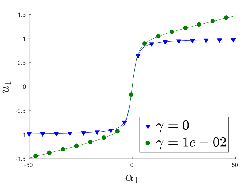
(a) Comparison of the maps (67) and (69) which relate the optimal first-order multiplier to the moment components for M₁ with Maxwell–Boltzmann statistics with $v_{0}=1$.

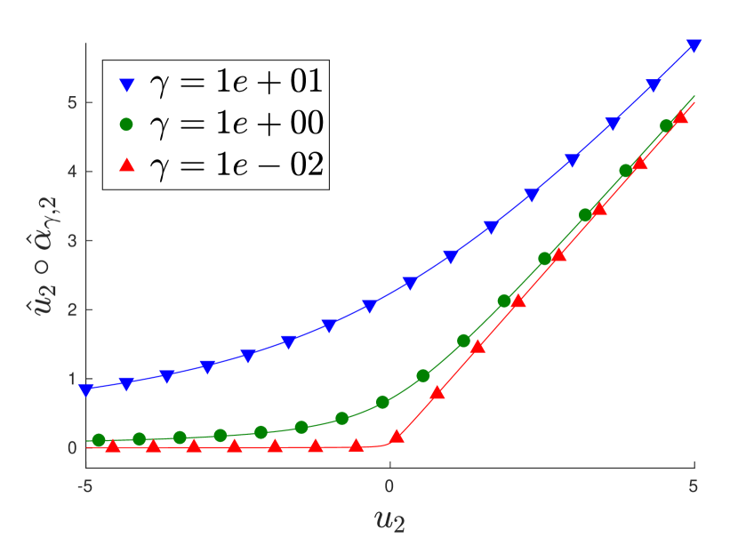
(b) Comparison of the regularized closures for $v_{2}$ of the Euler equations, given by (73). Here $v_{0}=1$ and $v_{1}=0$.

Figure 1: Comparison of regularized versus unregularized closures.

3.4.3 Regularized Euler equations

With $V=\mathbb{R}^{3}$ and $\mathbf{m}(v)=\{1,v,|v|^{2}\}$, the original entropy-based moment equation gives the compressible Euler equations [26]. In one-dimension, i.e., $V=\mathbb{R}$ and ${\mathbf{m}(v)=(1,v,v^{2})}$. The realizable set is $\mathcal{R}=\{(v_{0},v_{1},v_{2})\in\mathbb{R}^{3}:v_{0}v_{2}>v_{1}^{2}\}$. The moment and optimal multiplier components satisfy

$$v_{0} =\sqrt{-\frac{\pi}{\hat{\alpha}_{2}}}\exp\left(\hat{\alpha}_{0}-\frac{\hat{\alpha}_{1}^{2}}{4\hat{\alpha}_{2}}\right),$$ (70a)

$$v_{1} =\sqrt{-\frac{\pi}{\hat{\alpha}_{2}}}\exp\left(\hat{\alpha}_{0}-\frac{\hat{\alpha}_{1}^{2}}{4\hat{\alpha}_{2}}\right)\frac{-\hat{\alpha}_{1}}{2\hat{\alpha}_{2}},$$ (70b)

$$v_{2} =\sqrt{-\frac{\pi}{\hat{\alpha}_{2}}}\exp\left(\hat{\alpha}_{0}-\frac{\hat{\alpha}_{1}^{2}}{4\hat{\alpha}_{2}}\right)\left(\frac{\hat{\alpha}_{1}^{2}}{4\hat{\alpha}_{2}^{2}}-\frac{1}{2\hat{\alpha}_{2}}\right),$$ (70c)

and one can readily invert these equations.

Again, we have been unable to solve these equations analytically when all moment components are regularized. We were only able to find an analytical solution for the case when we only relax the equality constraint on $v_{2}$. In this case (70c) becomes

$$v_{2}=\sqrt{-\frac{\pi}{\hat{\alpha}_{\gamma,2}}}\exp\left(\hat{\alpha}_{\gamma,0}-\frac{\hat{\alpha}_{\gamma,1}^{2}}{4\hat{\alpha}_{\gamma,2}}\right)\left(\frac{\hat{\alpha}_{\gamma,1}^{2}}{4\hat{\alpha}_{\gamma,2}^{2}}-\frac{1}{2\hat{\alpha}_{\gamma,2}}\right)+\gamma\hat{\alpha}_{\gamma,2},$$ (71)

and with appropriate substitutions of (70a)–(70b) (with the multipliers now labeled with $\gamma$), we get

$$\hat{\alpha}_{\gamma,2}=\frac{v_{2}v_{0}-v_{1}^{2}-\sqrt{(v_{2}v_{0}-v_{1}^{2})^{2}+2\gamma v_{0}^{3}}}{2\gamma v_{0}}.$$ (72)

Then the regularized second-order moment becomes:

$$\hat{v}_{2}(\hat{\boldsymbol{\alpha}}_{\gamma}(\mathbf{v}))=v_{0}\left(\frac{v_{1}^{2}}{v_{0}^{2}}+\frac{v_{2}v_{0}-v_{1}^{2}+\sqrt{(v_{2}v_{0}-v_{1}^{2})^{2}+2\gamma v_{0}^{3}}}{2v_{0}^{2}}\right).$$ (73)

Figure 1(b) shows this relationship, and it behaves as expected: when $\gamma$ approaches zero, it approaches the identity map for positive $v_{2}$; otherwise, for nonphysical negative values of $v_{2}$, the map returns small positive values which get even smaller as $\gamma$ goes to zero.

4 Accuracy of the closure

While the properties in Section 3.2 provide basic structure of the regularized entropy-based moment equations (41), Theorem 1 hints at an attractive possible application: the use the regularized system to accurately solve the original moment system (21). To explore this idea further, we note that $\mathbf{f}_{\gamma}(\mathbf{v})=\mathbf{f}(\hat{\mathbf{v}}(\hat{\boldsymbol{\alpha}}_{\gamma}(\mathbf{v}))$, where $\hat{\mathbf{v}}(\hat{\boldsymbol{\alpha}}_{\gamma}(\mathbf{v}))\in\mathcal{R}$ is the regularization of $\mathbf{v}\in\mathbb{R}^{n}$. (Indeed, the term $\langle\mathbf{m}g\rangle$ in (40) is an approximate evaluation of $\hat{\mathbf{v}}\circ\hat{\boldsymbol{\alpha}}_{\gamma}$ at $\mathbf{v}^{\delta}$.) Thus under the assumption that the Jacobian of $\mathbf{f}$ is bounded, the moment mismatch $\hat{\mathbf{v}}(\hat{\boldsymbol{\alpha}}_{\gamma}(\mathbf{v}))-\mathbf{v}$ can be used to estimate $\mathbf{f}_{\gamma}(\mathbf{v})-\mathbf{f}(\mathbf{v})$. If the $\mathcal{O}(\delta)$-accuracy in Theorem 1 holds uniformly for all $\mathbf{v}\in\mathcal{R}$, then we can see $\mathbf{f}_{\gamma}$ as way to approximately, but accurately evaluate $\mathbf{f}$. The collision term $\mathbf{r}_{\gamma}$ can be considered similarly.

4.1 Accuracy of the moment regularization map

With the help of the relationships in Section 3.1, we can now analyze the moment regularization map $\hat{\mathbf{v}}\circ\hat{\boldsymbol{\alpha}}_{\gamma}$ directly.

Theorem 2.

Let

$$\mathbf{v}\in\mathcal{R}^{M}:=\{\mathbf{v}:\|\hat{\boldsymbol{\alpha}}(\mathbf{v})\|<M\},$$ (74)

and let $\mathbf{v}^{\delta}$ satisfy

$$\|\mathbf{v}^{\delta}-\mathbf{v}\|\leq\delta.$$ (75)

Then

$$\|\hat{\mathbf{v}}(\hat{\boldsymbol{\alpha}}_{\gamma}(\mathbf{v}^{\delta}))-\mathbf{v}\|\leq\delta+M\gamma.$$ (76)

Proof.

Let $\widetilde{\mathbf{v}}:=\hat{\mathbf{v}}_{\gamma}(\hat{\boldsymbol{\alpha}}(\mathbf{v}))$. Then $\mathbf{v}=\hat{\mathbf{v}}(\hat{\boldsymbol{\alpha}}_{\gamma}(\widetilde{\mathbf{v}}))$ so that

$$\left\|\hat{\mathbf{v}}(\hat{\boldsymbol{\alpha}}_{\gamma}(\mathbf{v}^{\delta}))-\mathbf{v}\right\| =\left\|\hat{\mathbf{v}}(\hat{\boldsymbol{\alpha}}_{\gamma}(\mathbf{v}^{\delta}))-\hat{\mathbf{v}}(\hat{\boldsymbol{\alpha}}_{\gamma}(\widetilde{\mathbf{v}}))\right\|$$ (77a)

$$=\left\|\int_{0}^{1}\left.\frac{\partial(\hat{\mathbf{v}}\circ\hat{\boldsymbol{\alpha}}_{\gamma})}{\partial\mathbf{v}}\right|_{\widetilde{\mathbf{v}}+s(\mathbf{v}^{\delta}-\widetilde{\mathbf{v}})}(\mathbf{v}^{\delta}-\widetilde{\mathbf{v}})\,ds\right\|$$ (77b)

$$=\left\|\int_{0}^{1}\left.H(\hat{\boldsymbol{\alpha}}_{\gamma})(H(\hat{\boldsymbol{\alpha}}_{\gamma})+\gamma I)^{-1}\right|_{\widetilde{\mathbf{v}}+s(\mathbf{v}^{\delta}-\widetilde{\mathbf{v}})}(\mathbf{v}^{\delta}-\widetilde{\mathbf{v}})\,ds\right\|$$ (77c)

$$\leq\int_{0}^{1}\left\|\left.H(\hat{\boldsymbol{\alpha}}_{\gamma})(H(\hat{\boldsymbol{\alpha}}_{\gamma})+\gamma I)^{-1}\right|_{\widetilde{\mathbf{v}}+s(\mathbf{v}^{\delta}-\widetilde{\mathbf{v}})}\right\|\,ds\|\mathbf{v}^{\delta}-\widetilde{\mathbf{v}}\|$$ (77d)

$$=\int_{0}^{1}\left.\frac{\|H(\hat{\boldsymbol{\alpha}}_{\gamma})\|}{\|H(\hat{\boldsymbol{\alpha}}_{\gamma})\|+\gamma}\right|_{\widetilde{\mathbf{v}}+s(\mathbf{v}^{\delta}-\widetilde{\mathbf{v}})}\,ds\|\mathbf{v}^{\delta}-\widetilde{\mathbf{v}}\|$$ (77e)

$$\leq\|\mathbf{v}^{\delta}-\widetilde{\mathbf{v}}\|.$$ (77f)

The inverse relationship between $\hat{\mathbf{v}}$ and $\hat{\boldsymbol{\alpha}}$, along with (45), gives

$$\mathbf{v}^{\delta}-\widetilde{\mathbf{v}}=(\mathbf{v}^{\delta}-\mathbf{v})+(\mathbf{v}-\widetilde{\mathbf{v}}) \stackrel{{\scriptstyle\hphantom{\eqref{eq:vhatg}}}}{{=}}(\mathbf{v}^{\delta}-\mathbf{v})+(\hat{\mathbf{v}}(\hat{\boldsymbol{\alpha}}(\mathbf{v}))-\hat{\mathbf{v}}_{\gamma}(\hat{\boldsymbol{\alpha}}(\mathbf{v})))$$

$$\stackrel{{\scriptstyle\eqref{eq:vhatg}}}{{=}}(\mathbf{v}^{\delta}-\mathbf{v})-\gamma\hat{\boldsymbol{\alpha}}(\mathbf{v})).$$ (78)

Altogether we have

$$\|\hat{\mathbf{v}}(\hat{\boldsymbol{\alpha}}_{\gamma}(\mathbf{v}^{\delta}))-\mathbf{v}\|\stackrel{{\scriptstyle\eqref{eq:udiff-int}}}{{\leq}}\|\mathbf{v}^{\delta}-\widetilde{\mathbf{v}}\|\stackrel{{\scriptstyle\eqref{eq:utilde-alpha}}}{{\leq}}\|\mathbf{v}^{\delta}-\mathbf{v}\|+\gamma\|\hat{\boldsymbol{\alpha}}(\mathbf{v})\| \stackrel{{\scriptstyle\eqref{eq:udelta}}}{{\leq}}\delta+\gamma\|\hat{\boldsymbol{\alpha}}(\mathbf{v})\|$$

$$\stackrel{{\scriptstyle\eqref{eq:RM}}}{{\leq}}\delta+M\gamma.$$ (79)

∎

As a result of Theorem 1, if $\gamma\leq C\delta$ for some $C\in(0,\infty)$, then the moment regularization error $\|\hat{\mathbf{v}}(\hat{\boldsymbol{\alpha}}_{\gamma}(\mathbf{v}^{\delta}))-\mathbf{v}\|$ is $\mathcal{O}(\delta)$. This result gives uniform accuracy over a large set of moment vectors, but only by bounding this set away from the boundary of the realizable set by controlling the norm of the associated multiplier vectors. The closer the moment vectors get to the boundary of the realizable set, the larger the constant in the error bound becomes.

4.2 Stopping criterion for the optimization

As in Theorem 1, we would like to use an approximate solution to the optimization problem while keeping $\mathcal{O}(\delta)$ accuracy. The error is quantified by the value of the primal objective function, but previous work with entropy-based moment methods has used the norm of the dual gradient for the stopping criterion (e.g., [1]). The norm of the dual gradient is preferable because it is already computed by the optimizer (as part of the search-direction computation) and is easy to interpret. We will show that these two stopping criteria are closely related, but first we give our result with the gradient-based criterion.

Theorem 3.

Assume $\mathbf{v}\in\mathcal{R}^{M}$; let $\mathbf{v}^{\delta}$ satisfy $\|\mathbf{v}^{\delta}-\mathbf{v}\|\leq\delta$; and let $\boldsymbol{\alpha}$ satisfy

$$\|\hat{\mathbf{v}}(\boldsymbol{\alpha})-\mathbf{v}^{\delta}+\gamma\boldsymbol{\alpha}\|\leq\tau.$$ (80)

Then

$$\|\hat{\mathbf{v}}(\boldsymbol{\alpha})-\mathbf{v}\|\leq 2\delta+M\gamma+2\tau.$$ (81)

Proof.

We write

$$\hat{\mathbf{v}}(\boldsymbol{\alpha})-\mathbf{v}=\hat{\mathbf{v}}(\boldsymbol{\alpha})-\mathbf{v}^{\delta}+\gamma\boldsymbol{\alpha}+(\mathbf{v}^{\delta}-\mathbf{v})-\gamma\boldsymbol{\alpha}.$$ (82)

and apply the triangle inequality, using (80), to find

$$\|\hat{\mathbf{v}}(\boldsymbol{\alpha})-\mathbf{v}\|\leq\tau+\delta+\gamma\|\boldsymbol{\alpha}\|.$$ (83)

To bound $\boldsymbol{\alpha}$, let $\widetilde{\mathbf{v}}:=\hat{\mathbf{v}}_{\gamma}(\boldsymbol{\alpha})=\hat{\mathbf{v}}(\boldsymbol{\alpha})+\gamma\boldsymbol{\alpha}$. Then

$$\|\widetilde{\mathbf{v}}-\mathbf{v}\|\leq\|\widetilde{\mathbf{v}}-\mathbf{v}^{\delta}\|+\|\mathbf{v}^{\delta}-\mathbf{v}\|\stackrel{{\scriptstyle\eqref{eq:stopping}}}{{\leq}}\tau+\delta$$ (84)

and, since $\boldsymbol{\alpha}=\hat{\boldsymbol{\alpha}}_{\gamma}(\widetilde{\mathbf{v}})$,

$$\boldsymbol{\alpha}=\hat{\boldsymbol{\alpha}}_{\gamma}(\mathbf{v})+\int_{0}^{1}(H(\hat{\boldsymbol{\alpha}}_{\gamma}(\mathbf{v}+s(\widetilde{\mathbf{v}}-\mathbf{v})))+\gamma I)^{-1}(\widetilde{\mathbf{v}}-\mathbf{v})\,ds.$$ (85)

Thus $\|\boldsymbol{\alpha}\|$ is bounded by

$$\|\boldsymbol{\alpha}\|\leq\|\hat{\boldsymbol{\alpha}}_{\gamma}(\mathbf{v})\|+\frac{1}{\gamma}\|\widetilde{\mathbf{v}}-\mathbf{v}\|\stackrel{{\scriptstyle\eqref{eq:vtilde_bound}}}{{\leq}}\|\hat{\boldsymbol{\alpha}}_{\gamma}(\mathbf{v})\|+\frac{\tau+\delta}{\gamma}.$$ (86)

The term $\|\hat{\boldsymbol{\alpha}}_{\gamma}(\mathbf{v})\|$ can be further bounded because $\|\hat{\boldsymbol{\alpha}}_{\gamma}(\mathbf{v})\|$ is a decreasing function of $\gamma$:

$$\frac{\partial}{\partial\gamma}\|\hat{\boldsymbol{\alpha}}_{\gamma}(\mathbf{v})\|^{2} =2\hat{\boldsymbol{\alpha}}_{\gamma}(\mathbf{v})\cdot\frac{\partial}{\partial\gamma}\hat{\boldsymbol{\alpha}}_{\gamma}(\mathbf{v})$$ (87a)

$$=2\hat{\boldsymbol{\alpha}}_{\gamma}(\mathbf{v})\cdot\left(-\left.\frac{\partial\hat{\mathbf{v}}_{\gamma}}{\partial\boldsymbol{\alpha}}\right|_{\hat{\boldsymbol{\alpha}}_{\gamma}(\mathbf{v})}\left.\frac{\partial\hat{\mathbf{v}}_{\gamma}}{\partial\gamma}\right|_{\hat{\boldsymbol{\alpha}}_{\gamma}(\mathbf{v})}\right)$$ (87b)

$$=-2\hat{\boldsymbol{\alpha}}_{\gamma}(\mathbf{v})\cdot((H_{\gamma}^{-1}(\hat{\boldsymbol{\alpha}}_{\gamma}(\mathbf{v}))\hat{\boldsymbol{\alpha}}_{\gamma}(\mathbf{v}))$$ (87c)

$$\leq 0,$$ (87d)

The derivative of $\hat{\boldsymbol{\alpha}}_{\gamma}$ with respect to $\gamma$ is computed by differentiating both sides of $\hat{\mathbf{v}}_{\gamma}(\hat{\boldsymbol{\alpha}}_{\gamma}(\mathbf{v}))=\mathbf{v}$ with respect to $\gamma$, as in the implicit function theorem. Since the continuity of $\hat{\boldsymbol{\alpha}}_{\gamma}$ with respect to $\gamma$ at $\gamma=0$ is a consequence of the same continuity of $\hat{\mathbf{v}}_{\gamma}$, we can extend (86) to

$$\|\boldsymbol{\alpha}\|\leq\|\hat{\boldsymbol{\alpha}}(\mathbf{v})\|+\frac{\tau+\delta}{\gamma}\leq M+\frac{\tau+\delta}{\gamma}.$$ (88)

Setting the bound (88) into (83) yields (81) ∎

If $\gamma\leq C\delta$ and $\tau\leq C^{\prime}\delta$, then the error $\|\hat{\mathbf{v}}(\boldsymbol{\alpha})-\mathbf{v}\|$ of the approximate projection is $\mathcal{O}(\delta)$. Thus we achieve a bound like that of Theorem 1 but with constants independent of the specific moment vectors $\mathbf{v}$ and $\mathbf{v}^{\delta}$, as long as $\mathbf{v}\in\mathcal{R}^{M}$.

We now turn to the relationship between the stopping criterion (80) and that of [14, 15]. In the latter, a distribution $g$ is called $\tau^{\prime}$-optimal if, for a given tolerance $\tau^{\prime}\in(0,\infty)$, it satisfies

$$\mathcal{H}(g)+\frac{1}{2\gamma}\left\|\left\langle\mathbf{m}g\right\rangle-\mathbf{v}\right\|^{2}\leq h_{\gamma}(\mathbf{v})+\tau^{\prime},$$ (89)

where $h_{\gamma}(\mathbf{v})$ is the infimum of $\mathcal{H}_{\gamma}(\cdot;\mathbf{v})$; see (43). Because $h_{\gamma}(\mathbf{v})$ is typically unknown, we cannot practically enforce (89) as is. However, we find a computable and stronger criterion by considering the duality gap [5, §5.5.1]. Indeed, for any $\boldsymbol{\alpha}$ we have (44)

$$\boldsymbol{\alpha}\cdot\mathbf{v}-\left\langle\eta_{*}(\boldsymbol{\alpha}\cdot\mathbf{m})\right\rangle-\frac{\gamma}{2}\|\boldsymbol{\alpha}\|^{2}\leq h_{\gamma}(\mathbf{v});$$ (90)

so if the multiplier vector $\boldsymbol{\alpha}$ further satisfies

$$\mathcal{H}(G_{\boldsymbol{\alpha}})+\frac{1}{2\gamma}\|\left\langle\mathbf{m}G_{\boldsymbol{\alpha}}\right\rangle-\mathbf{v}\|^{2}\leq\boldsymbol{\alpha}\cdot\mathbf{v}-\left\langle\eta_{*}(\boldsymbol{\alpha}\cdot\mathbf{m})\right\rangle-\frac{\gamma}{2}\|\boldsymbol{\alpha}\|^{2}+\tau^{\prime},$$ (91)

we can conclude that it satisfies (89). Since the optimal duality gap is zero, (91) can be achieved for any $\tau^{\prime}>0$.

Now, the form of $G_{\boldsymbol{\alpha}}$ and the fact that $\eta$ and $\eta_{\ast}$ are Legendre duals imply that

$$\eta(G_{\boldsymbol{\alpha}})+\eta_{*}(\boldsymbol{\alpha}\cdot\mathbf{m}) =\boldsymbol{\alpha}\cdot\mathbf{m}G_{\boldsymbol{\alpha}}.$$ (92)

This relation reduces (91) to

$$\frac{1}{2\gamma}\|\left\langle\mathbf{m}G_{\boldsymbol{\alpha}}\right\rangle-\mathbf{v}+\gamma\boldsymbol{\alpha}\|^{2}\leq\tau^{\prime}.$$ (93a)

which gives a stopping criterion equivalent to (80), where the tolerances are related by $\tau=\sqrt{2\gamma\tau^{\prime}}$.

4.3 Accuracy tests

To verify accuracy numerically, we consider the following curve in the realizable set:

$$\mathbf{u}(x):=\left\langle\mathbf{m}\exp(\alpha_{0}(x)+\alpha_{1}(x)\mu)\right\rangle,$$ (94)

where $x\in[-\pi,\pi]$ and

$$\alpha_{0}(x):=-\sin(x)+c\quad\mbox{and}\quad\alpha_{1}(x):=K+\sin(x).$$ (95a)

The parameter $K$ is used to move the moment curve closer to the boundary of the realizable set. The constant $c$ is set to

$$c =\log\left(\cfrac{K-1}{2\sinh(K-1)}\right)-1$$ (96)

so that $1=\max_{x}u_{0}(x)$.

We generate an error-contaminated moment vector $\mathbf{v}^{\delta}$ by projecting the moment curve on the interval $[0,\Delta x]$ onto the space of polynomials up to degree $k-1$. We let $\mathbf{u}_{\Delta x}(0)$ denote the evaluation at $x=0$ of the $(k-1)$-th degree polynomial projection of $\mathbf{u}(x)$ given in (94) on $[0,\Delta x]$. We choose the edge $x=0$ simply because it would appear in a finite-volume method.

The velocity space is $V=[-1,1]$ (as in the numerical tests in Section 5 below), and for the basis functions $\mathbf{m}$ we take the Legendre polynomials up to seventh order. We compute the velocity integrals in (94) using a forty-point Gauss–Lobatto quadrature and the spatial inner products for the orthogonal projection with a twenty-point Gauss–Lobatto quadrature.

In Table 2, we plot the error

$$\|\hat{\mathbf{v}}(\boldsymbol{\alpha}_{\gamma}^{\tau}(\mathbf{u}_{\Delta x}(0)))-\mathbf{u}(0)\|,$$ (97)

where $\boldsymbol{\alpha}_{\gamma}^{\tau}(\mathbf{u}_{\Delta x}(0)))$ denotes the first Newton iterate satisfying the stopping criterion (80) for the moment vector $\mathbf{u}_{\Delta x}(0)$. The test results confirm that the appropriate choices of $\gamma$ and $\tau$ give the expected orders of convergence. We note that almost all of the moment vectors $\mathbf{u}_{\Delta x}(0)$ generated by the polynomial projections for the table are not realizable.

	$k=2$		$k=3$		$k=4$
$\Delta x$	$E^{1}_{h}$	$\nu$	$E^{1}_{h}$	$\nu$	$E^{1}_{h}$	$\nu$
$2^{-1}$	5.7e-01		4.2e-01		2.8e-01
$2^{-2}$	2.8e-01	0.99	6.9e-02	2.62	1.5e-02	4.23
$2^{-3}$	6.9e-02	2.05	1.0e-02	2.77	1.3e-03	3.55
$2^{-4}$	1.5e-02	2.19	1.3e-03	2.97	7.5e-05	4.10
$2^{-5}$	4.5e-03	1.75	1.4e-04	3.18	4.8e-06	3.95
$2^{-6}$	1.3e-03	1.81	2.0e-05	2.83	3.1e-07	3.97
$2^{-7}$	3.2e-04	1.99	2.5e-06	3.02	1.9e-08	4.03
$2^{-8}$	7.5e-05	2.11	3.1e-07	3.00	1.1e-09	4.05
$2^{-9}$	2.0e-05	1.90	3.8e-08	3.03	7.3e-11	3.97

Table 2: Regularization errors for $K=200$ and $\gamma=\tau=\Delta x^{k}$.

5 Numerical results

In this section we demonstrate that (41) can be simulated using an off-the-shelf, high-order method for hyperbolic conservation laws. Our simulations indicate that the results of Section 4 can be used to guide the choice of the regularization parameter $\gamma$ and the optimization tolerance $\tau$ so that a numerical solution of (41) is an accurate solution of the original entropy-based moment system (21). We also present numerical simulations of a benchmark problem.

For numerical tests, we consider a kinetic equation that describes particles of unit speed moving through a material with slab geometry (see e.g., [27]):

$$\partial_{t}f+\mu\partial_{x}f+\sigma_{\mathrm{a}}f=\sigma_{\mathrm{s}}(\left\langle f\right\rangle-f)+S.$$ (98)

The spatial domain is $X=(x_{\rm L},x_{\rm R})$ is one-dimensional, and the velocity variable $\mu\in[-1,1]$ gives the cosine of the angle between the microscopic velocity and and the $x$-axis. The collision operator here is $\mathcal{C}(f):=\sigma_{\mathrm{s}}(\langle f\rangle-f)$, where $\sigma_{\mathrm{s}}\geq 0$ is the scattering cross section. This collision operator $\mathcal{C}$ represents isotropic scattering, is linear, and dissipates any convex entropy $\eta$. Our equation also has a loss term $\sigma_{\mathrm{a}}f$, where $\sigma_{\mathrm{a}}\geq 0$ is the absorption cross section, as well as a source $S=S(t,x,\mu)$. Equation (98) is supplemented with the initial conditions

$$f(0,x,\mu)=f_{0}(x,\mu)$$ (99)

and boundary conditions

$$f(t,x_{\rm L},\mu>0)=f_{\rm L}(t,\mu)\qquad\mbox{and}\qquad f(t,x_{\rm R},\mu<0)=f_{\rm R}(t,\mu).$$ (100)

The original entropy-based moment equations for (98) are

$$\partial_{t}\mathbf{u}+\partial_{x}\mathbf{f}(\mathbf{u})+\sigma_{\mathrm{a}}\mathbf{u}=\sigma_{\mathrm{s}}R\mathbf{u}+\mathbf{s},$$ (101)

where $R=\operatorname{diag}\{0,-1,\dots,-1\}$ and $\mathbf{s}:=\langle\mathbf{m}S\rangle$. The regularized entropy-based moment equations for (98) are

$$\partial_{t}\mathbf{u}+\partial_{x}\mathbf{f}_{\gamma}(\mathbf{u})+\sigma_{\mathrm{a}}\mathbf{u}=\sigma_{\mathrm{s}}R\hat{\mathbf{v}}(\hat{\boldsymbol{\alpha}}_{\gamma}(\mathbf{u}))+\mathbf{s}.$$ (102)

Remark 2.

To achieve the entropy-dissipation property described in Section 3.2, we must use the regularized moment vector $\hat{\mathbf{v}}(\hat{\boldsymbol{\alpha}}_{\gamma}(\mathbf{u}))$ in the collision operator. This makes the collision operator nonlinear. The absorption term is not part of the collision operator and thus not part of the entropy-dissipating structure of the kinetic equation (98), and for that reason we simply leave it as a linear decay term in the regularized moment equations.

The initial conditions are $\mathbf{u}(0,x)=\left\langle\mathbf{m}f_{0}(x,\cdot)\right\rangle$ and and to define the boundary conditions we extend the definitions of $f_{\rm L}$ and $f_{\rm R}$ from $\mu\in[0,1]$ and $\mu\in[-1,0]$ respectively to all $\mu\in[-1,1]$ to get

$$\mathbf{u}(t,x_{\rm L})=\mathbf{u}_{\rm L}(t):=\left\langle\mathbf{m}f_{\rm L}(t,\cdot)\right\rangle\quad\mbox{and}\quad\mathbf{u}(t,x_{\rm R})=\mathbf{u}_{\rm R}(t):=\left\langle\mathbf{m}f_{\rm R}(t,\cdot)\right\rangle.$$ (103)

While this is not technically correct (and proper treatment of boundary conditions for moment methods remains an open problem), we only consider problems where the boundary conditions have at most a negligible effect on the solution.

For our numerical tests we take the Maxwell–Boltzmann entropy because it has generic physical relevance and leads to a nonnegative entropy ansatz. We take the Legendre polynomials up to order $N$ for the basis functions in $\mathbf{m}$, and so the number of moment components is $n=N+1$.

5.1 Numerical method

Two common high-order methods for hyperbolic equations are the discontinuous-Galerkin (DG) [9, 10] and weighted-essentially-nonoscillatory (WENO) [37] methods. The main consideration in selecting a method is the number of times one must compute multipliers $\hat{\boldsymbol{\alpha}}_{\gamma}(\mathbf{u})$ via (38), since this is the most expensive part of the algorithm. For the hyperbolic component, WENO offers a more attractive choice, since it only requires multipliers at the cell edges (and cell means, if a characteristic transformation is performed) in order to compute fluxes. A DG algorithm, on the other hand, needs multipliers on a quadrature set in each cell in order to evaluate the volume term. However, for the regularized equations (102) the collision term is nonlinear, and thus both the WENO and DG methods must approximately integrate this term in space with a quadrature, and each quadrature evaluation requires knowledge of the multipliers. Thus the advantages of WENO over DG are lost. We therefore proceed with a DG implementation, a description of which (in the context of solving (101)) can be found in [2]. The implementation here is essentially the same, except that a realizability limiter is not needed.

As in [2] we use the Lax-Friedrichs numerical flux. The numerical dissipation constant is set to one because the eigenvalues of the flux $\mathbf{f}_{\gamma}$ have the bound

$$\lambda_{\max}\left(\frac{\partial\mathbf{f}_{\gamma}}{\partial\mathbf{v}}\right)\leq 1,$$ (104)

where $\lambda_{\max}$ denotes the maximum (in absolute value) eigenvalue. This is a straightforward extension of [2, Lemma 3.1]. We use SSP Runge–Kutta methods for time integration, specifically those given in [24]: for the second-order results, we use the $s$-stage method with ten stages; for the third-order results, we use the $r^{2}$-stage method with $r=4$; and for the fourth-order results, we use the ten-stage method. We use a regular grid with $N_{x}$ spatial cells with width $\Delta x=(x_{\rm R}-x_{\rm L})/N_{x}$. The DG basis consists of polynomials up to degree $k-1$ on each cell. We choose the time step as in [2]:

$$\Delta t=\frac{w_{Q}\Delta x}{1+w_{Q}\Delta x(\sigma_{\mathrm{a}}+\sigma_{\mathrm{s}})},$$ (105)

where $w_{Q}$ is the weight of the endpoints of the $Q$-point Gauss-Lobatto quadrature with $2Q-2\geq k$. While in [2] this time step was chosen in order to maintain realizability of the cell means, which is irrelevant to us, we found that trying to use smaller time steps quickly led to stability problems.

We solve dual optimization problem (38) using a Levenberg-Marquardt-type algorithm and the Armijo line search.

5.2 Convergence test using a manufactured solution

To test how accurately the numerical solution of (102) approximates the numerical solution of the original entropy-based moment equations (101), we used the method of manufactured solutions, in particular the one proposed in [2]: Let

$$\mathbf{w}(t,x):=\left\langle\mathbf{m}\exp(\alpha_{0}(t,x)+\alpha_{1}(t,x)\mu)\right\rangle,$$ (106)

where

$$\alpha_{0}(t,x):=-\sin(x-t)+4t+c\qquad\mbox{and}\qquad\alpha_{1}(t,x):=K+\sin(x-t).$$ (107)

As above, the parameter $K$ is used to move the moment curve closer to the boundary of the realizable set, and the constant $c$ is set to

$$c =\log\left(\cfrac{K-1}{2\sinh(K-1)}\right)-1-4t_{\rm f},$$ (108)

so that $1=\max_{t,x}w_{0}(t,x)$. The spatial domain is $X=(-\pi,\pi)$, and we take the final time $t_{\rm f}:=\pi/5$. We use periodic boundary conditions and include neither scattering nor absorption: $\sigma_{\mathrm{a}}=\sigma_{\mathrm{s}}=0$. Since the goal is to converge to the solution of the original entropy-based moment equations (101), we compute the source $s$ for the manufactured solution using $\mathbf{f}$ instead of $\mathbf{f}_{\gamma}$; that is, we set ${\mathbf{s}=\partial_{t}\mathbf{w}+\partial_{x}\mathbf{f}(\mathbf{w})}$.

Error is measured in the $L^{1}$ sense: Let $\mathbf{u}_{\Delta x}(t_{\rm f},x)$ denote the point-wise evaluation of the DG solution at the final time; we consider the errors only in the zeroth component, which are given by

$$e_{\Delta x}=\int_{x_{\rm L}}^{x_{\rm R}}|u_{\Delta x,0}(t_{\rm f},x)-w_{0}(t_{\rm f},x)|\,dx.$$ (109)

We approximate the integral with a twenty-point Gauss–Lobatto quadrature in each spatial cell. Results are given in Table 3; we used a factor $10^{-1}$ in front of the $\Delta x^{k}$ for $\gamma$ and $\tau$ (unlike in Section 4.3). With this factor, we see the expected orders of convergence for different values of $k$. For larger values of this factor, the observed convergence in our tests is slightly smaller than expected.

	$k=2$		$k=3$		$k=4$
$N_{x}$	$e_{\Delta x}$	$\nu$	$e_{\Delta x}$	$\nu$	$e_{\Delta x}$	$\nu$
10	1.7184e-01	–	6.9233e-02	–	9.3886e-03	–
20	1.1080e-01	0.63	6.6889e-03	3.37	2.9149e-04	5.01
40	2.9046e-02	1.93	1.2543e-03	2.41	4.6188e-05	2.66
80	7.6273e-03	1.93	1.7001e-04	2.88	5.9739e-06	2.95
160	2.2065e-03	1.79	2.3744e-05	2.84	4.7288e-07	3.66
320	5.5530e-04	1.99	3.0206e-06	2.97	3.0056e-08	3.98
640	1.4088e-04	1.98	3.8838e-07	2.96	1.9219e-09	3.97
1280	3.6005e-05	1.97	4.8748e-08	2.99	1.1919e-10	4.01

Table 3: Errors between numerical solutions of the regularized equations to the exact solution of the original equations for the manufactured-solution test. Here, $N=3$, $K=5$, and we use the regularization and optimization parameters $\gamma=\tau=10^{-1}\Delta x^{k}$.

5.3 Plane-source benchmark

The plane-source problem [17] tests how well a method handles strong spatial gradients and angular distributions with highly localized support. We use a slightly smoothed version of this problem in which an initial delta function in space is replaced by a narrow Gaussian. Even with this smoothing, solutions are rough and numerical convergence is slow.

The domain is $X=(-1.2,1.2)$, and the initial conditions are given by

$$f_{t=0}(x,\mu)=\max\left(\frac{\exp\left(-x^{2}/\Sigma^{2}\right)}{\Sigma},f_{\rm floor}\right),$$ (110)

where $\Sigma=0.01$, and $f_{\rm floor}=0.5\times 10^{-8}$ approximates a vacuum. (The ansatz with the Maxwell–Boltzmann entropy, which has the form $\exp(\boldsymbol{\alpha}\cdot\mathbf{m})$, cannot be exactly zero.) The boundary conditions $f_{\rm L}(t,\mu)\equiv f_{\rm R}(t,\mu)\equiv f_{\rm floor}$ are consistent with the analytical solution. We simulate the solution up to $t_{\rm f}=1$.

For the results in this section, we first found the smallest values of $\gamma$ and $\tau$ with which we could reliably compute numerical solutions of the regularized equations without the optimizer crashing. These values were $\gamma=10^{-6}$ and $\tau=10^{-7}$. Then with these values, we compute a very accurate, nearly converged numerical solution using the fourth-order DG method with 4000 spatial cells. We compare this solution with a high-resolution solution of the original entropy-based moment equations, which we generate using the second-order kinetic scheme of [1]. We use 13000 cells with the kinetic scheme and even for the slightly smoothed version of the problem considered here, we do have to use the technique of isotropic regularization for some moment vectors in the numerical solution (see [1] for details).

Figure 2(a) shows the results for $N=5$. In this figure, the solutions are indistinguishable, but in Figures 2(b) and 2(c), we zoom in on the solutions in two places to show that differences on the order of 0.01, or about 1%, remain. We computed solutions for other values of $N$ and found similar results.

To get some understanding of the effect of the value of $\gamma$ on the solutions, we also present numerical solutions to the plane-source problem with two larger values of $\gamma$. (We continue to use $\tau=10^{-7}$ and the fourth-order DG method with 4000 cells.) In Figure 2(d) we include the results using $\gamma=10^{-2}$. While for the larger value of $\gamma$ the first and third waves of the solution are larger in magnitude, the second wave is smaller and somewhat delayed. The front of the third wave is also slightly delayed. It seems to us that while increasing the value of $\gamma$ does not have a smoothing effect, it does seem to have a delaying effect like that predicted by the analysis of the regularized P_N equations in Section 3.4.1. The zoomed-in plots in Figures 2(e) and 2(f) include a third, intermediate value of $\gamma$ which confirms this observation.

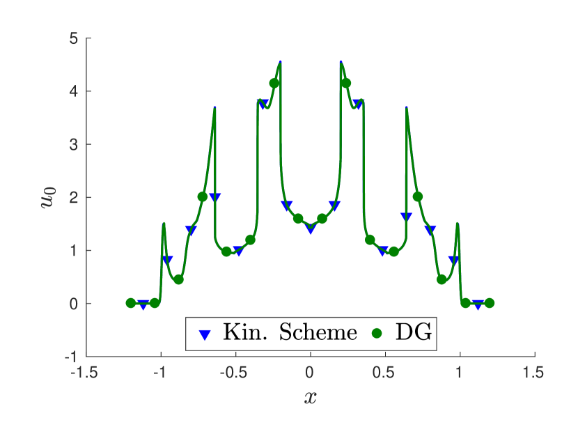
(a) Plane-source solution using the kinetic scheme and the fourth-order DG scheme with $\gamma=10^{-6}$.

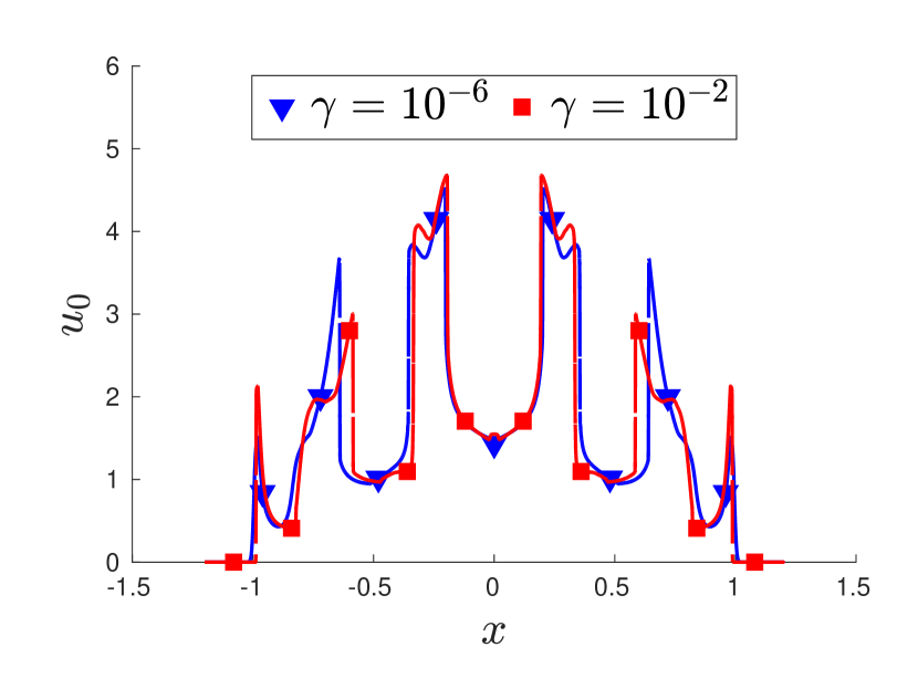
(d) Plane-source solution using two different values of $\gamma$.

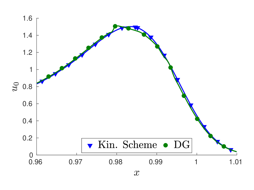
(b) Zoom-in around $x\in[0.96,1.01]$ of the comparison of the solutions from the old kinetic scheme and the new regularized equations.

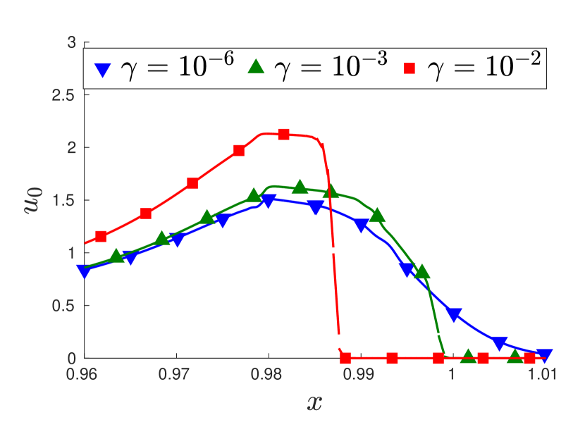
(e) Zoom-in around $x\in[0.96,1.01]$ of the comparison of the solutions for different values of $\gamma$.

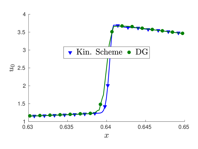
(c) Zoom-in around $x\in[0.63,0.65]$ of the comparison of the solutions from the old kinetic scheme and the new regularized equations.

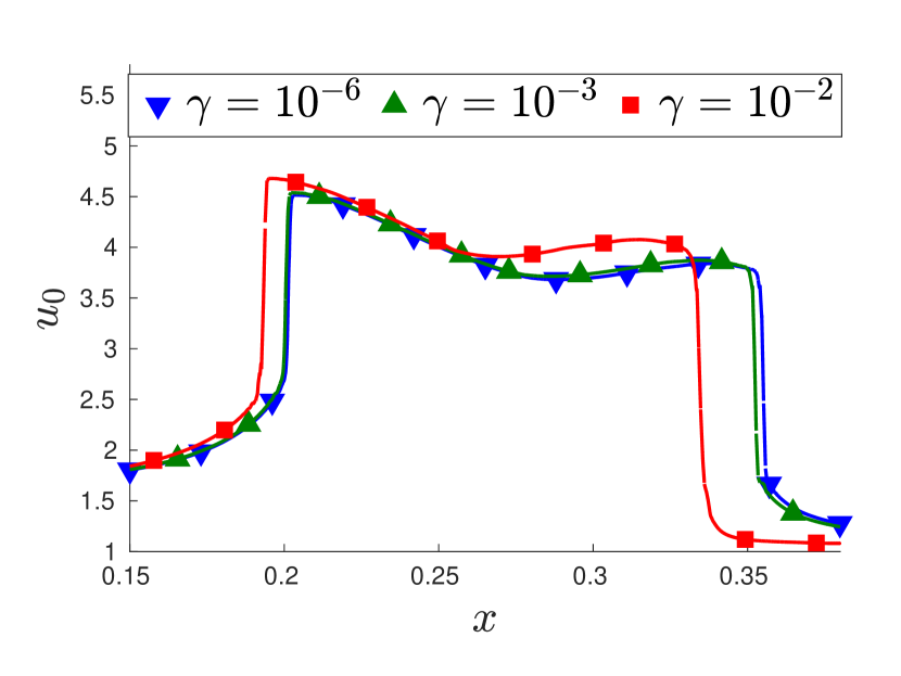
(f) Zoom-in around $x\in[0.15,0.4]$ of the comparison of the solutions for different values of $\gamma$.

Figure 2: Numerical solutions of the plane-source problem.

6 Concluding remarks

In this work we introduce a new moment method for kinetic equations. We derive this method, dubbed the regularized entropy-based moment method, by starting with the original entropy-based moment equations and relaxing the equality constraint in the optimization defining the ansatz reconstruction for the flux and collision terms. By relaxing these constraints, we can define flux and collision terms for nonrealizable moment vectors which, while unphysical, often appear as a result of discretization error in numerical simulations. The relaxation corresponds to a Tikhonov regularization in the defining optimization problem’s dual.

We showed that the regularized system keeps many of the same properties as the original system: Firstly, it dissipates entropy, albeit not the same as the original system but an approximation thereof, and is hyperbolic. When the basis functions are orthonormal, the regularized system is also rotationally symmetric. On the other hand, translational invariance is lost. The problem of degenerate densities for unbounded velocity domains also carries over to the regularized problem in the form of moment vectors for which the regularized problem has no solution.

We view these regularized equations as a tool to compute approximate solutions to the original entropy-based moment equations because the error in the regularized reconstruction can be controlled through the choice of the regularization parameter. Numerical simulations using a discontinuous-Galerkin (DG) scheme confirm this accuracy for the moment equations from a one-dimensional linear kinetic equation. We can use the DG scheme essentially off-the-shelf because relaxing the realizability requirement greatly simplifies its implementation.

For possible future work, a rigorous proof of the accuracy of the regularized equations would put the accuracy results on more solid ground. In one spatial dimension (where well-posedness theory for hyperbolic systems is available), perhaps the best route to this result is by examining the difference in the Jacobians of the fluxes $\mathbf{f}_{\gamma}$ and $\mathbf{f}$ and applying the results of [3].

The scheme could be improved by using an adaptive choice of the regularization parameter. Another improvement would be the development of an asymptotic-preserving scheme to handle stiff, collision-dominated kinetic regimes. This has been long sought for entropy-based moment equations, and we believe this will be more easily attainable without the obstacle of realizability.

Appendix A Degenerate densities

We recall that in Proposition 1 we are considering the Maxwell–Boltzmann entropy and $V=\mathbb{R}^{d}$. We let $\mathbf{m}$ contain polynomials up to degree $N$, for some even $N$, such that the only component of degree greater than or equal to $N$ is $m_{n-1}(v)=|v|^{N}$. Let $\mathcal{A}$ be the set of multiplier vectors such that $G_{\boldsymbol{\alpha}}\in L^{1}(V)$. In particular, we know that

$$\mathcal{A}\subset\{\boldsymbol{\alpha}\in\mathbb{R}^{n}:\alpha_{n-1}\leq 0\}\qquad\mbox{and}\qquad\mathcal{A}\cap\partial\mathcal{A}\subset\{\boldsymbol{\alpha}\in\mathbb{R}^{n}:\alpha_{n-1}=0\}.$$ (111)

In order to prove Proposition 1, we need the following lemma.

Lemma 1.

The function $\mathcal{H}_{\gamma}(\cdot;\mathbf{v})$ achieves a unique minimum if and only if $\mathbf{v}\in\hat{\mathbf{v}}_{\gamma}(\mathcal{A})$. The minimizer, if it exists, has the form $G_{\boldsymbol{\alpha}}$, defined in (17).

Proof.

First assume $\mathbf{v}=\hat{\mathbf{v}}_{\gamma}(\boldsymbol{\alpha})$ for some $\boldsymbol{\alpha}\in\mathcal{A}$. Since $\eta$ is convex,

$$\left\langle\eta(g)\right\rangle\geq\left\langle\eta(G_{\boldsymbol{\alpha}})\right\rangle+\left\langle\boldsymbol{\alpha}\cdot\mathbf{m}(g-G_{\boldsymbol{\alpha}})\right\rangle,$$ (112)

where we use the fact that $\eta^{\prime}(G_{\boldsymbol{\alpha}})=\boldsymbol{\alpha}\cdot\mathbf{m}$. Applying (112) to the definition of $\mathcal{H}_{\gamma}$ in (36) and using the fact that $\mathbf{v}=\left\langle\mathbf{m}G_{\boldsymbol{\alpha}}\right\rangle+\gamma\boldsymbol{\alpha}$ gives

$$\mathcal{H}_{\gamma}(g;\mathbf{v}) \geq\mathcal{H}_{\gamma}(G_{\boldsymbol{\alpha}};\mathbf{v})+\frac{1}{2\gamma}\|\langle\mathbf{m}g\rangle-\mathbf{v}\|^{2}-\frac{1}{2\gamma}\|\langle\mathbf{m}G_{\boldsymbol{\alpha}}\rangle-\mathbf{v}\|^{2}$$

$$\qquad+\left\langle\boldsymbol{\alpha}\cdot\mathbf{m}(g-G_{\boldsymbol{\alpha}})\right\rangle$$ (113a)

$$=\mathcal{H}_{\gamma}(G_{\boldsymbol{\alpha}};\mathbf{v})+\frac{1}{2\gamma}\|\langle\mathbf{m}g\rangle-\left\langle\mathbf{m}G_{\boldsymbol{\alpha}}\right\rangle-\gamma\boldsymbol{\alpha}\|^{2}-\frac{\gamma}{2}\|\boldsymbol{\alpha}\|^{2}$$

$$\qquad+\left\langle\boldsymbol{\alpha}\cdot\mathbf{m}(g-G_{\boldsymbol{\alpha}})\right\rangle$$ (113b)

$$=\mathcal{H}_{\gamma}(G_{\boldsymbol{\alpha}};\mathbf{v})+\frac{1}{2\gamma}\|\langle\mathbf{m}g\rangle-\left\langle\mathbf{m}G_{\boldsymbol{\alpha}}\right\rangle\|^{2}$$ (113c)

$$\geq\mathcal{H}_{\gamma}(G_{\boldsymbol{\alpha}};\mathbf{v}).$$ (113d)

Thus $G_{\boldsymbol{\alpha}}$ minimizes $\mathcal{H}_{\gamma}(\cdot;\mathbf{v})$.

On the other hand, assume $\mathcal{H}_{\gamma}(\cdot;\mathbf{v})$ has a minimizer, which we denote by $g^{*}$. The minimizer $g^{*}$ also solves the problem

$$\operatorname*{minimize}_{g\in\mathbb{F}(V)}\>\mathcal{H}_{\gamma}(g;\mathbf{v})\qquad\operatorname*{subject~{}to}\>\left\langle\mathbf{m}g\right\rangle=\left\langle\mathbf{m}g^{*}\right\rangle.$$ (114)

Moreover, because the penalty term in $\mathcal{H}_{\gamma}$ is constant on the constraint set in (114), $g^{*}$ solves the original problem (15) with $\mathbf{v}$ replaced by $\langle\mathbf{m}g^{*}\rangle$. Thus according to [18, Theorem 9], $g^{*}=G_{\boldsymbol{\alpha}}$ for some $\boldsymbol{\alpha}\in\mathcal{A}$.

Now let $\widetilde{g}\in L^{1}(V)$ be smooth and have compact support. We consider $\varepsilon$ small enough such that $G_{\boldsymbol{\alpha}}+\varepsilon\widetilde{g}\in\mathbb{F}(V)$. Since $G_{\boldsymbol{\alpha}}$ minimizes $\mathcal{H}_{\gamma}(\cdot;\mathbf{v})$, the Gateaux derivative of $\mathcal{H}_{\gamma}$ in the direction $\widetilde{g}$ must be zero, i.e.,

$$0 =\lim_{\varepsilon\to 0}\frac{d}{d\varepsilon}\mathcal{H}_{\gamma}(G_{\boldsymbol{\alpha}}+\varepsilon\widetilde{g};\mathbf{v})$$ (115a)

$$=\left\langle\eta^{\prime}(G_{\boldsymbol{\alpha}})\widetilde{g}\right\rangle+\frac{1}{\gamma}(\left\langle\mathbf{m}G_{\boldsymbol{\alpha}}\right\rangle-\mathbf{v})\cdot\left\langle\mathbf{m}\widetilde{g}\right\rangle$$ (115b)

$$=\left(\boldsymbol{\alpha}+\frac{1}{\gamma}(\left\langle\mathbf{m}G_{\boldsymbol{\alpha}}\right\rangle-\mathbf{v})\right)\cdot\left\langle\mathbf{m}\widetilde{g}\right\rangle,$$ (115c)

from which we can conclude, using the freedom in the choice of $\widetilde{g}$, that $\mathbf{v}=\hat{\mathbf{v}}_{\gamma}(\boldsymbol{\alpha})$. ∎

Remark 3.

Like the original problem, when $V$ is compact there are no degenerate densities. In this case, $\mathcal{A}=\mathbb{R}^{n}$, and since the dual of the regularized problem is strongly convex, it has a maximizer for any $\mathbf{v}\in\mathbb{R}^{n}$, and therefore $\hat{\mathbf{v}}(\mathcal{A})=\mathbb{R}^{n}$.

Proof of Proposition 1.

Let

$$\psi_{\gamma}(\boldsymbol{\alpha};\mathbf{v}):=\boldsymbol{\alpha}\cdot\mathbf{v}-\left\langle\eta_{\ast}(\boldsymbol{\alpha}\cdot\mathbf{m})\right\rangle-\frac{\gamma}{2}\|\boldsymbol{\alpha}\|^{2}$$ (116)

be the dual function for the regularized problem so that

$$\hat{\boldsymbol{\alpha}}_{\gamma}(\mathbf{v})=\operatorname*{argmax}_{\boldsymbol{\alpha}\in\mathcal{A}}\psi_{\gamma}(\boldsymbol{\alpha};\mathbf{v}).$$ (117)

One can extend the arguments from [18] to show that $\hat{\boldsymbol{\alpha}}_{\gamma}(\mathbf{v})$ exists for any $\mathbf{v}\in\mathbb{R}^{n}$ (although when $\hat{\boldsymbol{\alpha}}_{\gamma}(\mathbf{v})$ is on the boundary of $\mathcal{A}$, it may not satisfy the first-order necessary conditions, i.e., sometimes $\hat{\mathbf{v}}_{\gamma}(\hat{\boldsymbol{\alpha}}_{\gamma}(\mathbf{v}))\neq\mathbf{v}$).

Suppose that (35) has a minimizer $g^{*}$. Then by Lemma 1, $g^{*}=G_{\boldsymbol{\alpha}^{*}}$ with $\mathbf{v}=\hat{\mathbf{v}}_{\gamma}(\boldsymbol{\alpha}^{*})$. Since the latter shows that $\boldsymbol{\alpha}^{*}$ satisfies the first-order necessary conditions for (116) and $\psi_{\gamma}(\cdot;\mathbf{v})$ is strictly concave, we have $\boldsymbol{\alpha}^{*}=\hat{\boldsymbol{\alpha}}_{\gamma}(\mathbf{v})$. By rearranging terms in the first-order necessary conditions, we conclude ${\mathbf{v}-\gamma\hat{\boldsymbol{\alpha}}_{\gamma}(\mathbf{v})\in\hat{\mathbf{v}}(\mathcal{A})}$.

The contrapositive is: if $\mathbf{v}-\gamma\hat{\boldsymbol{\alpha}}_{\gamma}(\mathbf{v})\not\in\hat{\mathbf{v}}(\mathcal{A})$, then no minimizer exists. Thus our strategy is to show that when $\mathbf{v}$ has the form from (62), we have ${\mathbf{v}-\gamma\hat{\boldsymbol{\alpha}}_{\gamma}(\mathbf{v})\not\in\hat{\mathbf{v}}(\mathcal{A})}$.

First, note that when $\mathbf{v}$ has the form from (62), then the $\overline{\boldsymbol{\alpha}}$ must be $\hat{\boldsymbol{\alpha}}_{\gamma}(\mathbf{v})$. To see this, recognize that $\overline{\boldsymbol{\alpha}}\in\mathcal{A}\cap\partial\mathcal{A}$ implies that $\overline{\alpha}_{n-1}=0$, so that the concavity of $\psi_{\gamma}$ (and the requisite smoothness properties assured by [22, Lemma 5.2]) gives

$$\psi_{\gamma}(\boldsymbol{\alpha};\mathbf{v})\leq\psi_{\gamma}(\overline{\boldsymbol{\alpha}};\mathbf{v})+\psi^{\prime}_{\gamma}(\overline{\boldsymbol{\alpha}};\mathbf{v})\cdot(\boldsymbol{\alpha}-\overline{\boldsymbol{\alpha}})\stackrel{{\scriptstyle\eqref{eq:junk-form-g}}}{{=}}\psi_{\gamma}(\overline{\boldsymbol{\alpha}};\mathbf{v})+\delta\alpha_{n-1}\leq\psi_{\gamma}(\overline{\boldsymbol{\alpha}};\mathbf{v}).$$ (118)

Since the maximizer of $\psi_{\gamma}(\cdot;\mathbf{v})$ is unique, $\overline{\boldsymbol{\alpha}}=\hat{\boldsymbol{\alpha}}_{\gamma}(\mathbf{v})$. Thus (62) can be written as

$$\mathbf{v}-\gamma\hat{\boldsymbol{\alpha}}_{\gamma}(\mathbf{v})=\hat{\mathbf{v}}(\hat{\boldsymbol{\alpha}}_{\gamma}(\mathbf{v}))+\begin{pmatrix}0\\ \vdots\\ 0\\ \delta\end{pmatrix},$$ (119)

and by [22], the right-hand side is not in $\hat{\mathbf{v}}(\mathcal{A})$. ∎

With a little more work, one can show that all degenerate densities ${\mathbf{v}\in\mathbb{R}^{n}\setminus\hat{\mathbf{v}}_{\gamma}(\mathcal{A})}$ have the form (62). Furthermore, for the case of more general polynomial basis functions, one can extend the arguments of [18] to show that the regularized problem satisfies the analogous complimentary-slackness condition

$$\hat{\boldsymbol{\alpha}}_{\gamma}(\mathbf{v})\cdot(\mathbf{v}-\hat{\mathbf{v}}_{\gamma}(\hat{\boldsymbol{\alpha}}_{\gamma}(\mathbf{v})))=0.$$ (120)

This complementary-slackness condition is the key to characterizing the set degenerate densities (of the original problem) in [18]. Indeed, (120) can be used to show that the set of all degenerate densities for the regularized problem is a union of normal cones which has the same form as [18, Eq. (180)] with $\hat{\mathbf{v}}$ (in that paper’s notation, $\mathbf{r}$) replaced by $\hat{\mathbf{v}}_{\gamma}$.

References

- [1] G. Alldredge, C. Hauck, and A. Tits. High-order entropy-based closures for linear transport in slab geometry II: A computational study of the optimization problem. SIAM Journal on Scientific Computing, 34(4):B361–B391, 2012.
- [2] G. Alldredge and F. Schneider. A realizability-preserving discontinuous Galerkin scheme for entropy-based moment closures for linear kinetic equations in one space dimension. Journal of Computational Physics, 295:665–684, August 2015.
- [3] S. Bianchini and R. M. Colombo. On the stability of the standard Riemann semigroup. Proceedings of the American Mathematical Society, pages 1961–1973, 2002.
- [4] J. M. Borwein and A. S. Lewis. Duality relationships for entropy-like minimization problems. SIAM J. Control Optim., 1:191–205, 1991.
- [5] S. Boyd and L. Vandenberghe. Convex optimization. Cambridge University Press, 2004.
- [6] T. A. Brunner and J. P. Holloway. One-dimensional Riemann solvers and the maximum entropy closure. J. Quant. Spectrosc. Radiat. Transfer, 69:543–566, 2001.
- [7] Russel E. Caflisch and C. David Levermore. Equilibrium for radiation in a homogeneous plasma. The Physics of fluids, 29(3):748–752, 1986.
- [8] C. Cercignani. The Boltzmann Equation and Its Applications. Springer-Verlag New York, New York, 1988.
- [9] Bernardo Cockburn, George E. Karniadakis, and Chi-Wang Shu. Discontinuous Galerkin Methods: Theory, Computation and Applications. Springer-Verlag, 2000.
- [10] Bernardo Cockburn, San-Yih Lin, and Chi-Wang Shu. TVB Runge-Kutta local projection discontinuous Galerkin finite element method for conservation laws III: One-dimensional systems. Journal of Computational Physics, 84(1):90 – 113, 1989.
- [11] A. Decarreau, D. Hilhorst, C. Lemaréchal, and J. Navaza. Dual methods in entropy maximization. Application to some problems in crystallography. SIAM Journal on Optimization, 2(2):173–197, 1992.
- [12] Giacomo Dimarco and Lorenzo Pareschi. Asymptotic preserving implicit-explicit Runge–Kutta methods for nonlinear kinetic equations. SIAM Journal on Numerical Analysis, 51(2):1064–1087, 2013.
- [13] B. Dubroca and J.-L. Fuegas. Étude théorique et numérique d’une hiérarchie de modèles aus moments pour le transfert radiatif. C.R. Acad. Sci. Paris, I. 329:915–920, 1999.
- [14] H. W. Engl, K. Kunisch, and A. Neubauer. Convergence rates for Tikhonov regularisation of non-linear ill-posed problems. Inverse problems, 5(4):523–540, 1989.
- [15] H. W. Engl and G. Landl. Convergence rates for maximum entropy regularization. SIAM Journal on Numerical Analysis, 30(5):1509–1536, 1993.
- [16] L. C. Evans. Partial Differential Equations. Graduate studies in mathematics. American Mathematical Society, 2010.
- [17] B. D. Ganapol, P. W. McKenty, and K. L. Peddicord. The generation of time-dependent neutron transport solutions in infinite media. Nuclear Science and Engineering, 64(2):317–331, 1977.
- [18] Cory D. Hauck, C. David Levermore, and André L. Tits. Convex duality and entropy-based moment closures: Characterizing degenerate densities. SIAM J. Control Optim., 47(4):1977–2015, 2008.
- [19] Jingwei Hu, Ruiwen Shu, and Xiangxiong Zhang. Asymptotic-preserving and positivity-preserving implicit-explicit schemes for the stiff BGK equation. arXiv preprint arXiv:1708.06279, 2017.
- [20] Shi Jin. Efficient asymptotic-preserving (AP) schemes for some multiscale kinetic equations. SIAM Journal on Scientific Computing, 21(2):441–454, 1999.
- [21] M. Junk. Domain of definition of Levermore’s five moment system. J. Stat. Phys., 93(5-6):1143–1167, 1998.
- [22] M. Junk. Maximum entropy for reduced moment problems. Math. Meth. Mod. Appl. Sci., 10:1001–1025, 2000.
- [23] M. Junk and A. Unterreiter. Maximum entropy moment systems and Galilean invariance. Continuum Mech. Thermodyn., 14:563–576, 2002.
- [24] David I. Ketcheson. Highly efficient strong stability-preserving Runge–Kutta methods with low-storage implementations. SIAM Journal on Scientific Computing, 30(4):2113–2136, 2008.
- [25] J. B. Lasserre. Moments, Positive Polynomials and Their Applications. Imperial College Press, Singapore, 2010.
- [26] C. D. Levermore. Moment closure hierarchies for kinetic theories. J. Stat. Phys., 83:1021–1065, 1996.
- [27] E. E. Lewis and W. F. Miller, Jr. Computational Methods in Neutron Transport. John Wiley and Sons, New York, 1984.
- [28] Peter A. Markowich, Christian A. Ringhofer, and Christian Schmeiser. Semiconductor Equations. Springer-Verlag Wien, 1990.
- [29] Ryan G. McClarren, Thomas M. Evans, Robert B. Lowrie, and Jeffery D. Densmore. Semi-implicit time integration for thermal radiative transfer. Journal of Computational Physics, 227(16):7561–7586, 2008.
- [30] Ryan G. McClarren and Cory D. Hauck. Robust and accurate filtered spherical harmonics expansions for radiative transfer. Journal of Computational Physics, 229(16):5597–5614, 2010.
- [31] Ryan G. McClarren and Cory D. Hauck. Simulating radiative transfer with filtered spherical harmonics. Physics Letters A, 374(22):2290–2296, 2010.
- [32] Dimitri Mihalas and Barbara Weibel-Mihalas. Foundations of Radiation Hydrodynamics. Courier Corporation, 1999.
- [33] G. N. Minerbo. Maximum entropy Eddington factors. J. Quant. Spectrosc. Radiat. Transfer, 20:541–545, 1978.
- [34] E. Olbrant, C. D. Hauck, and M. Frank. A realizability-preserving discontinuous Galerkin method for the M1 model of radiative transfer. Journal of Computational Physics, 231(17):5612–5639, July 2012.
- [35] Florian Schneider, Graham Alldredge, and Jochen Kall. A realizability-preserving high-order kinetic scheme using WENO reconstruction for entropy-based moment closures of linear kinetic equations in slab geometry. Kinetic and Related Models, 9(1), 2016.
- [36] Jacques Schneider. Entropic approximation in kinetic theory. ESAIM: Mathematical Modelling and Numerical Analysis, 38(3):541–561, 2004.
- [37] Chi-Wang Shu. Essentially non-oscillatory and weighted essentially non-oscillatory schemes for hyperbolic conservation laws. In Alfio Quarteroni, editor, Advanced Numerical Approximation of Nonlinear Hyperbolic Equations, volume 1697 of Lecture Notes in Mathematics, pages 325–432. Springer Berlin Heidelberg, 1998.