One-dimensional backreacting holographic superconductors
with exponential nonlinear electrodynamics

Abstract

In this paper, we investigate the effects of nonlinear exponential electrodynamics as well as backreaction on the properties of one-dimensional $s$-wave holographic superconductors. We continue our study both analytically and numerically. In analytical study, we employ the Sturm-Liouville method while in numerical approach we perform the shooting method. We obtain a relation between the critical temperature and chemical potential analytically. Our results show a good agreement between analytical and numerical methods. We observe that the increase in the strength of both nonlinearity and backreaction parameters causes the formation of condensation in the black hole background harder and critical temperature lower. These results are consistent with those obtained for two dimensional $s$-wave holographic superconductors.

I Introduction

The $AdS/CFT$ duality provides a correspondence between a strongly coupled conformal field theory (CFT) in $d$-dimensions and a weakly coupled gravity theory in ($d+1$)-dimensional anti-de Sitter ($AdS$) spacetime 1 ; 2 ; 3 . Since it is a duality between two theories with different dimensions, it is commonly called holography. The idea of holography has been employed in condensed matter physics to study various phenomena such as superconductors 4 ; 5 ; 6 ; 7 ; 8 . For describing the properties of low temperature superconductors, the BCS theory can work very well 9 ; 10 . However, this theory fails to describe the mechanism of high temperature superconductor. In latter regime, the holography was suggested to study the properties of superconductors 11 ; 12 . Hortnol $et$ $al.$ have represented the first model of holographic superconductors 11 ; 12 . After that, holographic superconductors have attracted a lot of attention and investigated from different point of views 4 ; 13 ; 14 ; 15 ; 16 .

BTZ black holes play a significant role in many of recent developments in string theory 46 ; 47 ; 48 . BTZ-like solutions are dual of ($1+1$)-dimensional holographic systems such as one-dimensional holographic superconductors. Distinctive features of normal and superconducting phases of one-dimensional systems have been studied studied in 49 . The latter study was done in probe limit. Considering the effects of backreaction, the properties of one-dimensional holographic superconductors have been studied both numerically 50 ; 50-1 and analytically 51 ; 52 .

It is interesting to investigate the effect of nonlinear electrodynamic models on holographic systems including holographic superconductors 17 ; 18 ; 19 ; 20 ; 21 ; 22 ; 23 ; 24 ; 34 ; 30 ; 31 ; 32 ; 38 ; Doa ; n3 ; n5 ; n1 ; n2 ; n4 ; SheyPM . Nonlinear models carry more information than the usual Maxwell case and also are considered as a possible way for avoiding the singularity of the point-like charged particle at the origin 25 ; 26 ; 27 ; 28 ; 29 . The oldest nonlinear electrodynamic model is Born-Infeld (BI) model. There are also two BI-like nonlinear electrodynamics namely logarithmic 33 ; nn ; 34 and exponential 35 ; 36 ; n5 electrodynamics. It has been found that the exponential electrodynamics has stronger effect on the condensation than other models 37 .

In the present work, we will study the one-dimensional holographic superconductors both analytically and numerically in the presence of exponential electrodynamics. To bring rich physics in holographic model, we consider the backreaction of the scalar and gauge fields on the metric background 39 ; 40 ; 41 ; 42 ; 43 ; 44 ; 45 . To perform the analytical study, we employ the Sturm-Liouville eigenvalue problem. We will study the effects of nonlinear exponential electrodynamics model as well as backreaction on critical temperature. We shall also use the numerical shooting method to investigate the features of our holographic superconductors and make comparison between analytical and numerical results.

This paper is organized as follows: In next section, we introduce the action and basic field equations governing ($1+1$)-dimensional holographic superconductors in the presence of exponential electrodynamics. In section III, we study the properties of holographic superconductors applying the analytical method based on Sturm-Liuoville eigenvalue problem. In section IV, we study holographic superconductors numerically by employing the shooting method. We also compare our numerical and analytical results. Finally, in last section we will summarize our results.

II Holographic Set-up

To study a ($1+1$)-dimensional holographic superconductor, we consider a ($2+1$)-dimensional bulk action of AdS gravity coupled to a charged scalar field $\psi$

$$S = \frac{1}{2\kappa^{2}}\int d^{3}x\sqrt{-g}\left(R+\frac{2}{l^{2}}\right)$$

$$+\int d^{3}x\sqrt{-g}\left[L\left(F\right)-|\nabla\psi-iqA\psi|^{2}-m^{2}|\psi|^{2}\right],$$

where $g$ is the determinant of metric, $R$ is Ricci scalar, $l$ is the AdS radius, $A$ is electromagnetic potential and $F=F_{\mu\nu}F^{\mu\nu}$ in which $F_{\mu\nu}=\nabla_{[\mu}A_{\mu]}$. In action (LABEL:Act), $\kappa^{2}=8\pi G_{3}$ where $G_{3}$ is the ($2+1$)-dimensional Newtonian constant and $m$ and $q$ represent the mass and charge of scalar field, respectively. $L\left(F\right)$ stands for the Lagrangian of electrodynamics model. ($1+1$)-dimensional holographic superconductors in the presence of linear Maxwell electrodynamics presented by $L\left(F\right)=-F/4$ have been studied in 50 ; 53 . The linear model is an idealization of reality. In principle, other powers of $F$ may play role. There are different nonlinear electrodynamics models which exhibit the electrodynamics interaction. In this paper, we suppose that electrodynamics interaction is governed by exponential nonlinear electrodynamics model 35

$$L\left(F\right)=\frac{1}{4b}\left({\mathrm{e}}^{-bF}-1\right),$$ (2)

where $b$ determines the nonlinearity. For small values of $b$, Lagrangian (2) recovers the linear Maxwell Lagrangian. The parameter $\kappa$ in (LABEL:Act) also determines the backreaction. When $\kappa$ goes to zero, we are in the probe limit, meaning that the gravity part of action (LABEL:Act) is stronger than the matter field part. Physically, this implies that the gauge and matter fields do not back react on the metric background. In superconducting language, implies that the Cooper pairs have negligible interaction with background system. In the presence of backreaction, the dual black hole solution may be given by the ansatz

$$ds^{2}=-f(r){\mathrm{e}}^{-\chi(r)}dt^{2}+\frac{dr^{2}}{f(r)}+\frac{r^{2}}{l^{2}}dx^{2}.$$ (3)

The Hawking temperature of above black hole solution is given by

$$T=\frac{f^{\prime}(r_{+}){\mathrm{e}}^{-\chi(r_{+})}}{4\pi},$$ (4)

where $r_{+}$ is event horizon which could be obtained as the greatest root of $f(r)=0$. Varying the action (LABEL:Act) with respect to $\psi$, $A_{\nu}$ and $g_{\mu\nu}$, the field equations read, respectively,

$$0 = \left(\nabla_{\mu}-i{q}A_{\mu}\right)\left(\nabla^{\mu}-i{q}A^{\mu}\right)\psi-m^{2}\psi\,,$$ (5)

$$0 = \nabla^{\mu}\left(4L_{F}F_{\mu\nu}\right)$$ (6)

$$-i{q}\left[-\psi^{\ast}(\nabla_{\nu}-i{q}A_{\nu})\psi+\psi(\nabla_{\nu}+i{q}A_{\nu})\psi^{\ast}\right]\,,$$

$$0 = \frac{1}{2\kappa^{2}}\left[R_{\mu\nu}-g_{\mu\nu}\left(\frac{R}{2}+\frac{1}{l^{2}}\right)\right]+2F_{ac}F_{b}{}^{c}L_{F}$$

$$-\frac{g_{\mu\nu}}{2}\left[L\left(F\right)-m^{2}|\psi|^{2}-{|\nabla\psi-i{q}A\psi|^{2}}\right]$$

$$-\frac{1}{2}\left[(\nabla_{\mu}\psi-i{q}A_{\mu}\psi)(\nabla_{\nu}\psi^{\ast}+i{q}A_{\nu}\psi^{\ast})+\mu\leftrightarrow\nu\right],$$

where $L_{F}=\partial L/\partial F$. Adopting the ansatz $A_{\mu}=\phi(r)\delta_{\mu}^{0}$ and $\psi=\psi(r)$, field equations (5)-(LABEL:03) lead to

$$0 = \psi^{\prime\prime}+\psi^{\prime}\left[\frac{1}{r}+\frac{f^{\prime}}{f}-\frac{\chi^{\prime}}{2}\right]+\psi\left[\frac{q^{2}\phi^{2}{\mathrm{e}}^{\chi}}{f^{2}}-\frac{m^{2}}{f}\right],$$ (8)

$$0 = \phi^{\prime\prime}+\phi^{\prime}\left(\frac{1}{r}+\frac{\chi^{\prime}}{2}\right)$$ (9)

$$-{\frac{2{q}^{2}\psi^{2}\phi}{{\mathrm{e}^{2b\phi^{\prime 2}{\mathrm{e}^{\chi}}}}f}+2b\phi^{\prime 2}{\mathrm{e}^{\chi}}\left(2\phi^{\prime\prime}+\phi^{\prime}\chi^{\prime}\right)},$$

$$0 = f^{\prime}+{\frac{\kappa^{2}r}{2b}}\left[1+{\mathrm{e}^{2b\phi^{\prime 2}{\mathrm{e}^{\chi}}}}\left(4b\phi^{\prime 2}{\mathrm{e}^{\chi}}-1\right)\right]$$ (10)

$$+2\,\kappa^{2}r\left[{\frac{q^{2}\phi^{2}\psi^{2}{\mathrm{e}^{\chi}}}{f}}+\left(m\psi\right)^{2}+\psi^{\prime 2}f\right]-{\frac{2r}{{l}^{2}}},$$

$$0 = \chi^{\prime}+4\kappa^{2}r\left[\frac{q^{2}\phi^{2}\psi^{2}{\mathrm{e}}^{\chi}}{f^{2}}+\psi^{\prime 2}\right].$$ (11)

where the prime denotes the derivative with respect to $r$. Obviously, the above equations reduce to the corresponding equations in Ref. 50 when $b\rightarrow 0$ while in the absence of the backreaction ($\kappa\rightarrow 0$), Eqs. (LABEL:12) and (LABEL:13) reduce to ones in Ref. 37 . By virtue of symmetries of field equations (LABEL:12)-(25)

$$q\rightarrow q/a,\text{ \ \ \ \ }\phi\rightarrow a\phi,\text{ \ \ \ \ }\psi\rightarrow a\psi,$$

$$\kappa\rightarrow\kappa/a,\text{ \ \ \ \ }b\rightarrow b/a^{2},$$ (12)

$$l\rightarrow al,\text{ \ \ \ \ }r\rightarrow ar,\text{ \ \ \ \ }q\rightarrow q/a,$$

$$m\rightarrow m/a,\text{ \ \ \ \ }b\rightarrow a^{2}b,$$ (13)

one can set $q=l=1$. In the following sections, we will study the superconding phase transition both analytically and numerically.

III Analytical Study

The behaviors of model functions governed by field equations (LABEL:12)-(25) near the boundary $r\rightarrow\infty$ are

$$\chi(r)\rightarrow 0,\qquad f(r)\sim r^{2},$$

$$\phi(r)\sim\rho+\mu\ln(r),\qquad\psi(r)\sim\frac{\psi_{-}}{r^{\Delta_{-}}}+\frac{\psi_{+}}{r^{\Delta_{+}}},$$ (14)

where $\mu$ and $\rho$ are chemical potential and charge density of dual field theory and $\Delta_{\pm}=1+\sqrt{1\pm m^{2}}$. The superconducting phase transition is characterized by growing the expectation value of order parameter $\left\langle O\right\rangle$ as temperature decreases. In normal phase, $\left\langle O\right\rangle$ vanishes. According to holographic dictionary, the expectation value of order parameter $\left\langle O\right\rangle$ is dual to ${\psi_{+}}$ or ${\psi_{-}}$ while the other one can be considered as the source. Therefore, near the critical point $\left\langle O_{\pm}\right\rangle$ is small and one can define it as

$$\epsilon\equiv\left\langle O_{i}\right\rangle,$$ (15)

where $i=+$ or $-$. Since $\epsilon$ is so small, we can expand the model functions as 39 ; 54 ; 55 ; 56

$$f=f_{0}+\epsilon^{2}f_{2}+\epsilon^{4}f_{4}+\cdots,$$ (16)

$$\chi=\epsilon^{2}\chi_{2}+\epsilon^{4}\chi_{4}+\cdots,$$ (17)

$$\psi=\epsilon\psi_{1}+\epsilon^{3}\psi_{3}+\epsilon^{5}\psi_{5}+\cdots,$$ (18)

$$\phi=\phi_{0}+\epsilon^{2}\phi_{2}+\epsilon^{4}\phi_{4}+\cdots.$$ (19)

Also we can expand the chemical potential as 55

$$\mu=\mu_{0}+\epsilon^{2}\delta\mu_{2}+...,$$ (20)

where $\delta\mu_{2}>0$. Thus, the order parameter as a function of chemical potential can be obtained as

$$\epsilon\approx\frac{(\mu-\mu_{0})^{1/2}}{\delta\mu_{2}}.$$ (21)

When $\mu\rightarrow\mu_{0}$, phase transition occurs and the order parameter is zero at the critical value $\mu_{c}=\mu_{0}$. Above equation also indicates the critical exponent $\beta=1/2$ which is the same as the universal result from the mean field theory. Hereafter, we define the dimensionless coordinate $z=r_{+}/r$ instead of $r,$ since it is easier to work with it. In terms of this new coordinate, $z=0$ and $z=1$ correspond to the boundary and horizon respectively. The field equations (LABEL:12)-(25) can be rewritten in terms of $z$ as

$$0 = \psi^{\prime\prime}+\left[\frac{1}{z}+\frac{f^{\prime}}{f}-\frac{\chi^{\prime}}{2}\right]\psi^{\prime}+\frac{r_{+}^{2}}{z^{4}}\left[\frac{q^{2}\phi^{2}{\mathrm{e}}^{\chi}}{f^{2}}-\frac{m^{2}}{f}\right]\psi,$$

$$0 = \phi^{\prime\prime}+\left(\frac{\chi^{\prime}}{2}+\frac{1}{z}\left[\frac{1+4\Upsilon}{1+2\Upsilon}\right]\right)\phi^{\prime}-\frac{2q^{2}r_{+}^{2}\psi^{2}}{z^{4}f}\left(\frac{{\mathrm{e}}^{-\Upsilon}}{1+2\Upsilon}\right)\phi,$$

$$0 = f^{\prime}-{\frac{\kappa^{2}{r_{+}}^{2}}{2bz^{3}}}\left[1+{\mathrm{e}^{\Upsilon}}\left({2\Upsilon}-1\right)\right]$$ (24)

$$-\frac{2\kappa^{2}{r_{+}^{2}}}{z^{3}}\left[\frac{q^{2}\phi^{2}{\psi^{2}}{\mathrm{e}^{\chi}}}{f}+m^{2}\psi^{2}\right]+{\frac{2{r_{+}^{2}}}{z^{3}}},$$

$$0 = \chi^{\prime}-\frac{4\kappa^{2}r_{+}^{2}}{z^{3}}\left[\frac{q^{2}\phi^{2}\psi^{2}{\mathrm{e}}^{\chi}}{f^{2}}+\frac{z^{4}\psi^{\prime 2}}{r_{+}^{2}}\right],$$ (25)

where $\Upsilon=2bz^{4}{\mathrm{e}}^{\chi}\phi^{\prime 2}/{r_{+}}^{2}$. The field equation of $\phi$ (Eq. (LABEL:13)) at zeroth order with respect to $\epsilon$ reduces to

$$\phi^{\prime\prime}(z)+\frac{\phi^{\prime}(z)(r_{+}^{2}+8{b}{z^{4}}\phi^{\prime 2}(z))}{z(r_{+}^{2}+4{b}{z^{4}}\phi^{\prime 2}(z))}=0.$$ (26)

The solution of above equation reads

$$\phi(z)=\int_{1}^{z}\frac{r_{+}\sqrt{L_{W}(\frac{4bz^{2}C_{0}^{2}}{{r_{+}}^{2}})}}{2{z^{2}}\sqrt{b}}dz,$$ (27)

where $C_{0}$ is an integration constant and $L_{W}(x)=LambertW(x)$ is the Lambert function which satisfies 57

$$L_{W}(x){\mathrm{e}}^{L_{W}(x)}=x,$$ (28)

and can be expanded as

$$L_{W}(x)=x-x^{2}+\frac{3}{2}x^{3}-\frac{8}{3}x^{4}.$$ (29)

Expanding Eq. (27) for small $b$ and keeping the terms up to first order of $b$ we find

$$\phi(z)=C_{1}+C_{0}\ln(z)+\frac{C_{0}^{3}}{r_{+}^{2}}(1-z^{2})b+O\left(b^{2}\right).$$ (30)

Comparing the above equation with Eq. (14), we find $C_{0}=-\mu$. Also, $C_{1}=0$, since at the horizon $\phi(r_{+})=0$. Inserting $C_{0}$ into Eq. (30) we have

$$\phi_{0}(z)=\lambda r_{+}\left[-\ln(z)+\lambda^{2}(z^{2}-1)b\right],\text{ \ \ \ \ }{b}\lambda^{2}<1,$$ (31)

where $\lambda=\mu/r_{+}$. Substituting $\phi(z)$ into the field equation (24), we find the metric function at zeroth order with respect to $\epsilon$, $f_{0}(z)=r_{+}^{2}g(z)$ where

$$g(z)=\left(\frac{1}{z^{2}}-1+\kappa^{2}\lambda^{2}\ln(z)+\frac{1}{2}\kappa^{2}\lambda^{4}b(1-z^{2})\right).$$ (32)

Note that at the horizon $f_{0}(1)=0$. The asymptotic behavior of scalar field $\psi$ near the boundary ($z=0$) is given by Eq. (14). In order to match this behavior near the boundary, we introduce a trial function $F(z)$ as $\psi(z)=\left\langle O_{i}\right\rangle\left(z/r_{+}\right)^{\Delta_{i}}F(z)$ which satisfies the boundary condition $F(0)=1$ and $F^{\prime}(0)=0$. Inserting the functions obtained above and the trial function $F(z)$ into Eq. (LABEL:12), one receives

$$F^{\prime\prime}(z)+F^{\prime}(z)\left[\frac{2\Delta+1}{z}+\frac{g^{\prime}(z)}{g(z)}\right]$$

$$+\left[-\frac{m^{2}}{g(z)z^{4}}+\frac{\Delta^{2}}{z^{2}}+\frac{\Delta g^{\prime}(z)}{zg(z)}\right]F(z)+$$

$$+\frac{q^{2}\lambda^{2}F(z)}{g(z)^{2}}\left[\frac{{\ln(z)}^{2}}{z^{4}}-\frac{2\lambda^{2}{b}{\ln(z)}}{z^{2}}+\frac{2\lambda^{2}{b}{\ln(z)}}{z^{4}}\right]=0.$$ (33)

It is a matter of calculations to show that the above equation satisfies the following second order Sturm-Liouville equation 58

$$\left[T(z)F^{\prime}(z)\right]^{\prime}-Q(z)F(z)+\lambda^{2}P(z)F(z)=0,$$ (34)

where

$$T(z) = {g(z)}z^{2\Delta+1},$$ (35)

$$P(z) = \frac{q^{2}T(z)}{g^{2}(z)}\left[\frac{{\ln(z)}^{2}}{z^{4}}-\frac{2\lambda^{2}{b}{\ln(z)}}{z^{2}}+\frac{2\lambda^{2}{b}{\ln(z)}}{z^{4}}\right],$$

$$Q(z) = -T(z)\left[-\frac{m^{2}}{g(z)z^{4}}+\frac{\Delta^{2}}{z^{2}}+\frac{\Delta g^{\prime}(z)}{zg(z)}\right].$$ (37)

Considering the trial function as $F(z)=1-\alpha z^{2}$ and using the Sturm-Liouville eigenvalues problem, the eigenvalues of Eq. (34) can be obtained by minimizing

$$\lambda^{2}=\frac{\int_{0}^{1}{dz}T(z)\left[F^{\prime 2}(z)+Q(z)F^{2}(z)\right]}{\int_{0}^{1}{dz}.T(z)P(z)F^{2}(z)},$$ (38)

with respect to $\alpha$ 59 . Here, we use a perturbative expansion $b\lambda^{2}$ up to the first order of $b$

$$b\lambda^{2}=b(\lambda^{2}|_{b=0})+O(b^{2}).$$ (39)

For backreaction parameter, we use iteration method and take

$$\kappa_{n}=n\Delta\kappa,\qquad\ n=0,1,2,3,\cdots,$$ (40)

where $\Delta\kappa=\kappa_{n+1}-\kappa_{n}$. Here we chose $\Delta\kappa=0.005$. So, the effect of the nonlinear corrections on the backreaction term can be obtained as

$$\kappa^{2}\lambda^{2}={\kappa_{n}}^{2}\lambda^{2}={\kappa_{n}}^{2}(\lambda^{2}|_{\kappa_{n-1}})+O[(\Delta\kappa)^{4}].$$ (41)

By taking $\kappa_{-1}=0$ and $\lambda^{2}|_{\kappa_{-1}}=0$, the minimum eigenvalue of Eq. (38) can be calculated. To calculate the critical temperature, we obtain the latter value by variation of Eq. (38) with respect to $\alpha$ where the other parameters such as $b,\kappa,m,q,\cdots$ are fixed. Using the definition of $T$ (Eq. (4)), the critical temperature is given by $T_{c}=f^{\prime}(r_{+})/4\pi$ where

$$f^{\prime}(r_{+})={{2{r_{+}}}}-{\frac{\kappa^{2}{r_{+}}}{2b}}\left[1+{\mathrm{e}^{2b\phi_{0}^{\prime 2}(r_{+})}}\left(4b\phi_{0}^{\prime 2}(r_{+})-1\right)\right],$$ (42)

and $r_{+}=\mu/\lambda$ so we have

$$T_{c}=\frac{1}{4\pi}\frac{\mu}{\lambda}\left[2-{\kappa_{n}}^{2}(\lambda^{2}|_{\kappa_{n-1}})+3b{\kappa_{n}}^{2}(\lambda^{4}|_{\kappa_{n-1},b=0})\right].$$ (43)

As an example, for $b=0.01$ and $\kappa=0$ the equation (38) reduce to

$$\lambda^{2}=\frac{0.667\alpha^{2}-1.333\alpha+1}{0.0276-0.0165\alpha+0.0035\alpha^{2}},$$ (44)

which has a minimum $\lambda_{\min}=21.6337$, with respect to $\alpha$, at $\alpha=0.8258$ and thus according to Eq. (43) we achieve $T_{c}=0.03421\mu$. We employ the iteration method to obtain the critical temperature for different values of $\kappa$ and $b$.

In table 1, we present our results. This table shows that by increasing nonlinear parameter ($b$), the value of $T_{c}$ decreases. As it can be understood from this table, for a fixed value of $b$, with increasing the backreaction parameter $\kappa$, the value of the critical temperature decreases. We also reproduce the results of the linear Maxwell case without backreaction (i.e. $b\rightarrow 0$ and $\kappa\rightarrow 0$) presented in 51 .

$b$	$\kappa^{2}=0$	$\kappa^{2}=0.005$	$\kappa^{2}=0.01$	$\kappa^{2}=0.015$	$\kappa^{2}=0.02$
0	0.0429	0.0393	0.0379	0.0369	0.0359
0.01	0.0342	0.0321	0.0311	0.0301	0.0288
0.02	0.0274	0.0231	0.0216	0.0208	0.0199

Table 1: Analytical results of ${T_{c}}/{\mu}$ for different values of $\kappa$ and $b$.

$b$	$\kappa^{2}=0$	$\kappa^{2}=0.05$	$\kappa^{2}=0.1$	$\kappa^{2}=0.15$	$\kappa^{2}=0.2$
0	0.046	0.0368	0.0295	0.0236	0.0189
0.01	0.0415	0.033	0.0262	0.0209	0.0166
0.04	0.0325	0.0252	0.0197	0.0154	0.0121
0.09	0.0236	0.0176	0.0133	0.0107	0.0078

Table 2: Numerical results of ${T_{c}}/{\mu}$ for different values of $\kappa$ and $b$.

IV Numerical Study

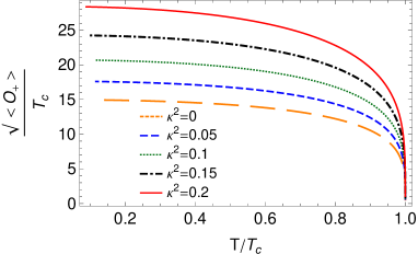
(a)  $b=0$

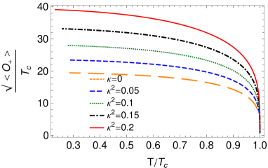
(b)  $b=0.04$

Figure 1: The behavior of order parameter versus temperature for $m^{2}=0$.

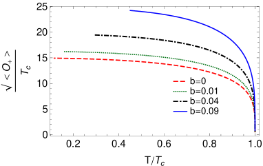
(a)  $\kappa^{2}=0$

(b)  $\kappa^{2}=0.1$

Figure 2: The behavior of order parameter versus temperature for $m^{2}=0$.

	$\kappa^{2}=0$		$\kappa^{2}=0.005$		$\kappa^{2}=0.01$		$\kappa^{2}=0.015$		$\kappa^{2}=0.02$
$b$	$T_{c}$(An)	$T_{c}$(Nu)	$T_{c}$(An)	$T_{c}$(Nu)	$T_{c}$(An)	$T_{c}$(Nu)	$T_{c}$(An)	$T_{c}$(Nu)	$T_{c}$(An)	$T_{c}$(Nu)
0	0.0429	0.046	0.0393	0.0449	0.0379	0.0439	0.0369	0.0430	0.0359	0.0409
0.01	0.0342	0.0415	0.0321	0.0406	0.0311	0.0396	0.0301	0.0387	0.0288	0.0378
0.02	0.0274	0.0380	0.0231	0.0371	0.0216	0.0362	0.0208	0.0353	0.0199	0.0345

Table 3: Analytical and numerical results of ${T_{c}}/{\mu}$ for different values of $\kappa$ and $b$.

In this section, we employ the shooting method 4 to numerically investigate the superconducting phase transition. Besides setting $q$ and $l$ to unity, we also set $r_{+}=1$ in the numerical calculation which may be justified by virtue of the field equation symmetry 50

$$r\rightarrow ar,\text{ \ \ \ \ }f\rightarrow a^{2}f,\text{ \ \ \ \ }\phi\rightarrow a\phi,$$

First, we expand Eqs. (LABEL:12)-(25) near black hole horizon ($z=1$)

$$\psi \approx \psi(1)+\psi^{\prime}(1)(1-z)+\frac{\psi^{{\prime}{\prime}}}{2}(1-z)^{2}+\cdots,$$ (45)

$$\phi \approx \phi^{\prime}(1)(1-z)+\frac{\phi^{{\prime}{\prime}}}{2}(1-z)^{2}+\cdots,$$ (46)

$$f \approx f^{\prime}(1)(1-z)+\frac{f^{{\prime}{\prime}}}{2}(1-z)^{2}+\cdots,$$ (47)

$$\chi \approx \chi(1)+\chi^{\prime}(1)(1-z)+\frac{\chi^{{\prime}{\prime}}}{2}(1-z)^{2}+\cdots.$$ (48)

In above equations, we have imposed $f(1)=\phi(1)=0$. In our numerical process, we will find $\psi(1)$, $\phi^{\prime}(1)$ and $\chi(1)$ such that the desired values for boundary parameters in Eq. (14) are attained. At boundary, one can set either $\psi_{-}$ or $\psi_{+}$ to zero as source and find the value of the other one as the expectation value of order parameter $\left\langle O\right\rangle$. We will focus on $m^{2}=0$ case for our numerical calculations. For this case, the behavior of $\psi$ near boundary is (see Eq. (14))

$$\psi(z)\approx\psi_{-}+{\psi_{+}}{z^{2}}.$$ (49)

We consider $\psi_{+}$ as holographic dual to the order parameter $\left\langle O_{+}\right\rangle$ at the boundary field theory.

In table 2, our numerical results for critical temperature with different values of backreaction parameter $\kappa$ and nonlinear parameter $b$ are presented. In the Maxwell limit ($b\rightarrow 0)$, our numerical results reproduce the ones of 50 . It can be seen that in the absence of nonlinearity effect, the critical temperature decreases as $\kappa$ increases 50 . In the presence of nonlinearity parameter i.e. for any nonvanishing value of $b$, it can be found that as $\kappa$ enhances, the critical temperature $T_{c}$ decreases. Similar behavior can be found for different values of $b$ when $\kappa$ is fixed. As the nonlinear parameter $b$ becomes larger, the critical temperature decreases i.e. the condensation process becomes harder. This behavior have been reported previously in 60 for ($2+1$)-dimensional holographic superconductors too. Figs. 1 and 2 confirm above results. As it can be seen from Fig. 1, the scalar hair forms harder as $\kappa$ increases i.e. the gap in graph of $\left\langle O_{+}\right\rangle$ becomes larger. The latter means that the condensation of the operator $\left\langle O_{+}\right\rangle$ starts at larger values for stronger values of backreaction parameter. It shows that the scalar hair can be formed more difficult when the backreaction is stronger. Fig. 2 shows the same effect for nonlinearity parameter $b$. We compare the analytical and numerical results in table 3. Table 3 shows that there is a good agreement between analytical and numerical results for small values of $\kappa$ and $b$. For larger values of these parameters, analytical and numerical results separate more from each other.

V Conclusion

In this work, we have studied the properties of one-dimensional holographic superconductor in the presence of nonlinear exponential electrodynamics. We have also considered the backreaction effect of scalar and gauge fields on the background metric. We have performed both analytical and numerical methods for studying our superconductors. To investigate the problem analytically, we have used the Sturm-Lioville while our numerical study was based on shooting method. It was shown that the enhancement in both nonlinearity of electrodynamics model as well as the backreaction causes the superconducting phase more difficult to be appeared. This result is reflected in two ways from our data. From one side, we observed that the increasement in the effects of nonlinearity and backreaction makes the critical temperature of superconductor lower. From another side, for larger values of nonlinear and backreaction parameters, the gap in condensation parameter is larger which in turn exhibits that the condensation is formed harder. We have also observed that, for small values of backreaction parameter $\kappa$ and nonlinear parameter $b$, the analytic results are in a good agreement with numerical ones whereas for larger values they separate more from each other.

Finally, we would like to stress that in this work, we have only studied the basic properties of one-dimensional backreacting holographic $s$-wave superconductors in the presence of exponential nonlinear electrodynamics. It is also interesting to investigate other characteristics of these systems such as the behaviour of real and imaginary parts of conductivity or optical features. One may also consider $(1+1)$-dimensional $p$-wave and $d$-wave holographic superconductors in the background of BTZ black holes and disclose the effects of nonlinearity as well as backreaction on the the phase transition and conductivity of these models. These issue are now under investigations and the result will be appeared soon.

- (1) J. M. Maldacena,The large-N limit of superconformal field theories and supergravity, Adv. Theor. Math. Phys. 2, 231 (1998) [arXiv:9711200].
- (2) S. S. Gubser, I. R. Klebanov and A. M. Polyakov, Gauge theory correlators from non-critical string theory, Phys. Lett. B 428, 105 (1998) [arXiv:9802109].
- (3) E. Witten, Anti-de Sitter space and holography, Adv. Theor. Math. Phys. 2, 253 (1998) [arXiv:9802150].
- (4) S. A. Hartnoll, Lectures on holographic methods for condensed matter physics, Class. Quant. Grav. 26, 224002 (2009) [arXiv:0903.3246].
- (5) C. P. Herzog, Lectures on Holographic Superfluidity and Superconductivity, J. Phys. A 42, 343001 (2009) [arXiv:0904.1975].
- (6) J. McGreevy, Holographic duality with a view toward many-body physics, Adv. High Energy Phys. 2010, 723105 (2010) [arXiv:0909.0518].
- (7) C. P. Herzog, Analytic holographic superconductor, Phys. Rev. D 81, 126009 (2010) [arXiv:1003.3278].
- (8) S. S. Gubser, Breaking an Abelian gauge symmetry near a black hole horizon, Phys. Rev. D 78, 065034 (2008) [arXiv:0801.2977]
- (9) J. Bardeen, L.N. Cooper and J. R. Schrieffer, Microscopic Theory of Superconductivity, Phys. Rev. 106, 162 (1957).
- (10) J. Bardeen, L. N. Cooper and J. R. Schrieffer, Theory of Superconductivity, Phys. Rev. 108, 1175 (1957).
- (11) S. A. Hartnoll, C. P. Herzog and G. T. Horowitz, Building a Holographic Superconductor, Phys. Rev. Lett. 101, 031601 (2008) [arXiv:0803.3295].
- (12) S. A. Hartnoll, C. P. Herzog and G. T. Horowitz, Holographic superconductors, JHEP 12, 015 (2008) [arXiv:0810.1563].
- (13) G. T. Horowitz and M. M. Roberts, Holographic Superconductors with Various Condensates, Phys. Rev. D 78, 126008 (2008) [arXiv:0810.1077].
- (14) S. Franco, A. Garcia-Garcia and D. Rodriguez-Gomez, A general class of holographic superconductors, JHEP 04, 092 (2010) [arXiv:0906.1214].
- (15) Q. Y. Pan and B. Wang, General holographic superconductor models with Gauss-Bonnet corrections, Phys. Lett. B 693, 159 (2010) [arXiv:1005.4743].
- (16) X. H. Ge, B. Wang, S. F. Wu and G. H. Yang, Analytical study on holographic superconductors in external magnetic field, JHEP 08, 108 (2010) [arXiv:1002.4901].
- (17) K. Skenderis, Black Holes and Branes in String Theory, Lect. Notes Phys. 541, 325 (2000) [arXiv:9901050].
- (18) S. Hyun, U-duality between Three and Higher Dimensional Black Holes, J. Kor. Phys. Soc. 33, S532 (1998) [arXiv:9704005].
- (19) A. Strominger, Black Hole Entropy from Near Horizon Microstates, JHEP 9802, 009 (1998) [arXiv:9712251].
- (20) J. Ren, One-dimensional holographic superconductor from / correspondence, JHEP 1011 , 055 (2010) [arXiv:1008.3904].
- (21) Y. Liu, Q. Pan and B. Wang, Holographic superconductor developed in BTZ black hole background with backreactions, Phys. Lett. B 702, 94 (2011) [arXiv:1106.4353].
- (22) M. Kord Zangeneh, Y. C. Ong and B. Wang, Entanglement entropy and complexity for one-dimensional holographic superconductors, Phys. Lett. B 771, 235 (2017) [arXiv:1704.00557].
- (23) R. Li, Note on analytical studies of one dimensional holographic superconductors, Mod. Phys. Lett. A 27, 1250001 (2012).
- (24) D. Momeni, M. Raza, M. R. Setare and R. Myrzakulov, Analytical holographic superconductor with backreaction using , Int. J. Theor. Phys. 52, 2773 (2013) [arXiv:1305.5163].
- (25) Y. Liu, Y. Peng and B. Wang, Gauss-Bonnet holographic superconductors in Born-Infeld electrodynamics with backreactions, arXiv:1202.3586.
- (26) Y. Liu, Y. Gong and B. Wang, Non-equilibrium condensation process in holographic superconductor with nonlinear electrodynamics, JHEP 02, 116 (2016) [arXiv:1505.03603].
- (27) D. Roychowdhury, Effect of external magnetic field on holographic superconductors in presence of non-linear corrections, Phys. Rev. D 86, 106009 (2012) [arXiv:1211.0904].
- (28) J. Jing and S. Chen, Holographic superconductors in the Born-Infeld electrodynamics, Phys. Lett. B 686, 68 (2010) [arXiv:1001.4227].
- (29) R. Banerjee, S. Gangopadhyay, D. Roychowdhury and A. Lala, Holographic s-wave condensate with nonlinear electrodynamics: A nontrivial boundary value problem, Phys. Rev. D 87, 104001 (2013) [arXiv:1208.5902].
- (30) J. Jing, Q. Pan and S. Chen, Holographic Superconductors with Power-Maxwell field, JHEP 11, 045 (2011) [arXiv:1106.5181].
- (31) Y. Liu and B. Wang, Perturbations around the AdS Born-Infeld black holes, Phys. Rev. D 85, 046011 (2012) [arXiv:1111.6729].
- (32) A. Sheykhi, H. R. Salahi and A. Montakhab, Analytical and Numerical Study of Gauss-Bonnet Holographic Superconductors with Power-Maxwell Field, JHEP 04, 058 (2016) [arXiv:1603.00075].
- (33) J. Jing, Q. Pan and S. Chen, Holographic superconductor/insulator transition with logarithmic electromagnetic field in Gausse Bonnet gravity, Phys. Lett. B 716, 385 (2012) [arXiv:1209.0893].
- (34) C. Lai, Q. Pan, J. Jing and Y. Wang, On analytical study of holographic superconductors with Born-Infeld electrodynamics, Phys. Lett. B 749, 437 (2015) [arXiv:1508.05926].
- (35) A. Sheykhi and F. Shaker, Analytical study of holographic superconductor in Born-Infeld electrodynamics with backreaction, Phys. Lett. B 754, 281 (2016) [arXiv:1601.04035].
- (36) S. Gangopadhyay, Holographic superconductors in Born-Infeld electrodynamics and external magnetic field, Mod. Phys. Lett. A 29, 1450088 (2014) [arXiv:1311.4416].
- (37) A. Sheykhi, A. Ghazanfari and A. Dehyadegari, Holographic conductivity of holographic superconductors with higher order corrections, Eur. Phys. J. C 78, 159 (2018) [arXiv:1712.04331].
- (38) A. Sheykhi, D. Hashemi Asl and A. Dehyadegari, Conductivity of higher dimensional holographic superconductors with nonlinear electrodynamics, Phys. Lett. B 781, 139 (2018) [arXiv:1803.05724].
- (39) M. Kord Zangeneh, S. S. Hashemi, A. Dehyadegari, A. Sheykhi and B. Wang, Optical properties of Born-Infeld-dilaton-Lifshitz holographic superconductors, arXiv:1710.10162.
- (40) Z. Sherkatghanad, B. Mirza and F. Lalehgani Dezaki, Exponential nonlinear electrodynamics and backreaction effects on holographic superconductor in the lifshitz black hole background, Int. J. Mod. Phys. D 27, 1750175 (2017) [arXiv:1708.04289].
- (41) A. Dehyadegari, M. Kord Zangeneh and A. Sheykhi, Holographic conductivity in the massive gravity with power-law Maxwell field, Phys. Lett. B 773, 344 (2017) [arXiv:1703.00975].
- (42) A. Dehyadegari, A. Sheykhi and M. Kord Zangeneh, Holographic Conductivity for Logarithmic Charged Dilaton-Lifshitz Solutions, Phys. Lett. B 758, 226 (2016) [arXiv:1602.08476].
- (43) M. Kord Zangeneh, A. Dehyadegari, A. Sheykhi and M. H. Dehghani, Thermodynamics and gauge/gravity duality for Lifshitz black holes in the presence of exponential electrodynamics, JHEP 1603, 037 (2016) [arXiv:1601.04732].
- (44) A. Sheykhi, F. Shamsi, S. Davatolhagh The upper critical magnetic field of holographic superconductor with conformally invariant Power–Maxwell electrodynamics, Can. J. Phys. 95, 450 (2017) [arXiv:1609.05040].
- (45) M. Born and L. Infeld, Foundations of the New Field Theory, Proc. R. Soc. A 144, 425 (1934).
- (46) B. Hoffmann, Gravitational and electromagnetic mass in the Born-Infeld electrodynamics, Phys. Rev. 47, 877 (1935).
- (47) W. Heisenberg and H. Euler, Z., Consequences of Dirac Theory of the Positron, Phys. 98, 714 (1936) [arXiv:0605038].
- (48) H. P. de Oliveira, Non-linear charged black holes, Class. Quant. Grav. 11, 1469 (1994).
- (49) G. W. Gibbons and D. A. Rasheed, Electric-magnetic duality rotations in non-linear electrodynamics, Nucl. Phys. B 454, 185 (1995) [arXiv:9506035].
- (50) H. H. Soleng, Charged black points in general relativity coupled to the logarithmic U(1) gauge theory, Phys. Rev. D 52, 6176 (1995) [arXiv:9509033].
- (51) A. Sheykhi, M. H. Dehghani and M. Kord Zangeneh, Thermodynamics of charged rotating dilaton black branes coupled to logarithmic nonlinear electrodynamics, Adv. High Energy Phys. 2016, 3265968 (2016) [arXiv:1604.05300].
- (52) S. H. Hendi, Asymptotic charged BTZ black hole solutions, JHEP 1203, 065 (2012) [arXiv:1405.4941].
- (53) S. H. Hendi and A. Sheykhi, Charged rotating black string in gravitating nonlinear electromagnetic fields, Phys. Rev. D 88, 044044 (2013) [arXiv:1405.6998].
- (54) Z. Zhao, Q. Pan, S. Chen and J. Jing, Notes on holographic superconductor models with the nonlinear electrodynamics, Nucl. Phys. 871, 98 (2013) [arXiv:1212.6693].
- (55) Q. Pan, J. Jing, B. Wang and S. Chen, Analytical study on holographic superconductors with backreactions, JHEP 06, 087 (2012) [arXiv:1205.3543].
- (56) S. S. Gubser and A. Nellore, Low-temperature behavior of the Abelian Higgs model in anti-de Sitter space, JHEP 04, 008 (2009) [arXiv:0810.4554].
- (57) Y. Brihaye and B. Hartmann, Holographic Superconductors in 3+1 dimensions away from the probe limit, Phys. Rev. D 81, 126008 (2010) [arXiv:1003.5130].
- (58) G. T. Horowitz and B. Way, Complete Phase Diagrams for a Holographic Superconductor/Insulator System, JHEP 11, 011 (2010) [arXiv:1007.3714].
- (59) A. Akhavan and M. Alishahiha, P-Wave Holographic Insulator/Superconductor Phase Transition, Phys. Rev. D 83, 086003 (2011) [arXiv:1011.6158].
- (60) S. Gangopadhyay, Analytic study of properties of holographic superconductors away from the probe limit, Phys. Lett. B 724, 176 (2013) [arXiv:1302.1288].
- (61) T. Konstandin, G. Nardini and M. Quiros, Gravitational Backreaction Effects on the Holographic Phase Transition, Phys. Rev. D 82, 083513 (2010) [arXiv:1007.1468].
- (62) J. Ren, One-dimensional holographic superconductor from correspondence, JHEP 1011, 055 (2010) [arXiv:1008.3904].
- (63) S. Kanno, A Note on Gauss-Bonnet Holographic Superconductors, Class. Quant. Grav. 28, 127001 (2011) [arXiv:1103.5022].
- (64) C. P. Herzog, Analytic holographic superconductor, Phys. Rev. D 81, 126009 (2010) [arXiv:1003.3278].
- (65) Xian-Hui GE and Hong-Qiang LENG, Analytical calculation on critical magnetic field in holographic superconductors with backreaction, Prog. Theor. Phys. 128, 1211 (2012) [arXiv:1105.4333].
- (66) M. Abramowitz and I. A. Stegun, Handbook of Mathematical Functions, Dover, New York, (1972).
- (67) S. Gangopadhyay and D. Roychowdhury, Analytic study of properties of holographic superconductors in Born-Infeld electrodynamics, JHEP 05, 002 (2012) [arXiv:1201.6520].
- (68) G. Siopsis and J. Therrien, Analytical calculation of properties of holographic superconductors, JHEP 1005, 013 (2010) [arXiv:1003.4275].
- (69) A. Sheykhi and F. Shaker, Effects of backreaction and exponential nonlinear electrodynamics on the holographic superconductors, Int. J. M. Phys. D 26, 1750050 (2017) [arXiv:1606.04364].