Simultaneous disease mapping and hot spot detection with application to childhood obesity surveillance from electronic health records

Abstract

Electronic health records (EHRs) have become a platform for data-driven surveillance on a granular level in recent years. In this paper, we make use of EHRs for early prevention of childhood obesity. The proposed method simultaneously provides smooth disease mapping and outlier information for obesity prevalence, which are useful for raising public awareness and facilitating targeted intervention. More precisely, we consider a penalized multilevel generalized linear model. We decompose regional contribution into smooth and sparse signals, which are automatically identified by a combination of fusion and sparse penalties imposed on the likelihood function. In addition, we weigh the proposed likelihood to account for the missingness and potential non-representativeness arising from the EHR data. We develop a novel alternating minimization algorithm, which is computationally efficient, easy to implement, and guarantees convergence. Simulation studies demonstrate superior performance of the proposed method. Finally, we apply our method to the University of Wisconsin Population Health Information Exchange database.

Keywords: Childhood obesity surveillance; disease mapping; electronic health records; fusion penalty; outlier detection; sparse penalty.

1 Introduction

Childhood obesity prevention has become increasingly important to control the global obesity pandemic. Granular-level surveillance of childhood obesity that identifies and tracks obesity trends is needed to help design interventions and guide policy solutions when monetary resources are limited. [Longjohn et al., 2010]. Several efforts have been made to construct local surveillance systems [Hoelscher et al., 2017], which are primarily school-based [Blondin et al., 2016]. Although school-based surveillance can be effective for data collection and implementation, there are concerns about privacy, stigmatization, and dysfunctional behavioral responses [Mass. Dep. Public Health, 2014]. Alternatively, routinely collected massive health databases such as Electronic Health Records (EHRs) are gaining attention as a platform for assessing trends and local childhood obesity risk [Friedman et al., 2013].

Statistical methods for geospatial surveillance may include two aspects: i) monitoring regional trends in prevalence (also known as “disease mapping” or “risk mapping”) and ii) identifying unexpected variation in the prevalence of different locations (also known as “hot spot detection”). Traditionally, these two tasks have been accomplished separately.

For task i), obesity literature mainly utilized the standard generalized linear mixed effect model (GLMM) to account for individual factors and community environments [Zhang et al., 2011, Davila-Payan et al., 2015]. Those approaches assumed the regional random effects to be independent, although a spatial dependency exists even after adjusting for covariates [Panczak et al., 2016]. To account for the spatial dependence, methods for smooth disease mapping have been proposed from both frequentist and Bayesian perspectives. Under Poisson log-linear models or multilevel logistic models, the region-specific effects were smoothed by kernels [Ghosh et al., 1999] or splines [Ugarte et al., 2010, Maiti et al., 2016], or were modeled as a dependent random vector by conditional autoregressive (CAR) priors [Waller et al., 1997, Pascutto et al., 2000, Lee, 2013, Mercer et al., 2015]. These strategies resulted in “clustered” risk maps, which enhanced interpretability, but did not explore identification of aberrant regions. For task ii), the most popular approach for detecting locations with outbreaking incidence is the spatial scan statistics approach [Kulldorff and Nagarwalla, 1995, Kulldorff, 1997, Jung, 2009]. The scan statistic methods search over a pre-specified set of geographical districts and conduct a generalized likelihood ratio test for testing whether the proportions of events are homogeneous across, inside, and outside the district. However, it may not be suitable for identifying multiple locations with heterogeneous sizes. Residuals generated from regression approaches can also be used to detect regional outbreaks [Kafadar and Stroup, 1992, Farrington et al., 1996, Zhao et al., 2011]. However, residual-based outlier detection is known to fail when an outlier is a leverage point or there are multiple outliers [She and Owen, 2011].

Use of the fusion penalty for smoothing was first proposed in a least squares setup [Tibshirani et al., 2005]. The resulting fit from the fusion penalty appears to be piecewise constant, yielding a natural clustering of fitted values. Smoothing by the fusion penalty enables an additional regularization using a different penalty, such as a sparse penalty, which may not be straightforward in other smooth disease mapping methods. Sparse penalty for outlier detection was used with the squared error loss [Kim et al., 2009, Tibshirani and Taylor, 2011, She and Owen, 2011]. Kim et al., [2009] and Tibshirani and Taylor, [2011] considered the $\ell_{1}$ penalty, and She and Owen, [2011] reported that nonconvex penalties outperformed both $\ell_{1}$ penalty and residual-based approaches for detection in standard multiple linear regression.

In this paper, we develop a new method that simultaneously produces an interpretable disease map and detects outlier regions. We formulate a multilevel logistic model to naturally incorporate risk factors. A novel hybrid regularization is introduced, where the region-specific effect is represented by the summation of a smooth signal and a sparse signal. The smooth signal is regularized by a fusion penalty so that adjacent locations tend to have similar fitted baseline obesity rates. A nonconvex sparse penalty is enforced for the sparse signals so that nonzero fitted coefficients signify potential outliers. It is worthwhile mentioning that estimating population health metrics from EHRs can be particularly challenging. First, subjects in EHRs systems are not randomly sampled. EHRs only capture people seeking healthcare. Second, recorded data often suffers from missingness, because for each patient, EHRs only collect data on the tests and conditions that clinicians order and diagnose. Thus, statistical models utilizing EHRs should deal with missingness and non-representativeness. Following Flood et al., [2015], we adopt a two-step weighting procedure to account for missing data and to adjust the covariate distribution for a nationally representative sample. We develop an alternating minimization algorithm to optimize a nonconvex objective function, which is computationally efficient and can leverage off-the-shelf software packages.

Our original contributions are twofold. First, while the hybrid regularization of the fusion and $\ell_{1}$ penalties has been considered in linear models [Kim et al., 2009, Tibshirani and Taylor, 2011], to the best of our knowledge, we are the first to incorporate a fusion penalty and a nonconvex penalty to identify outliers. Second, we provide an efficient optimization algorithm that guarantees convergence for the hybrid regularization model. Although our algorithm is described in a Bernoulli likelihood, it can be easily extended to handle other convex loss functions.

In Section 2, we introduce the University of Wisconsin Electronic Health Record Public Health Information Exchange (PHINEX) database that motivated our study. We introduce our model and formalize the objective function in Section 3. We also develop a computational algorithm and discuss tuning parameter selection in this section. Simulation studies are presented in Section 4, which demonstrate the superior performance of our proposed method. We apply our method to PHINEX on childhood obesity surveillance in Section 5. We provide concluding remarks in Section 6.

2 Data

The University of Wisconsin Electronic Health Record Public Health Information Exchange (UW eHealth PHINEX) database contains EHR data from a south-central Wisconsin academic healthcare system. It consists of patient records with documented primary care encounters at family medicine, pediatric, and internal medicine clinics occurring from 2007 to 2012. All PHINEX data were derived from the Epic EHR Clarity Database (EpicCare Electronic Medical Record, Epic Systems Corp., Verona WI). Furthermore, the program geocodes to the census blockgroup and links EHRs with community-level social determinants of health. It was created to improve clinical practice and population health by understanding local variations in disease risk, patients, and communities [Guilbert et al., 2012].

In this paper, we focused on 93,130 patients aged 2–19 years during 2011–2012. Body mass index (BMI) values (in $kg/m^{2}$) were calculated from a subject’s height and weight, measured at the same visit. Any subject with a BMI at or above the 95th percentile was categorized as obese. Among all the patients, 34,852 (37.4%) were missing a valid BMI. Subject covariates included sex, age, race/ethnicity, health service payer (i.e., insurance), and the 2010 census blockgroup information on subject residence. Economic hardship index (EHI) [Nathan and Adams, 1989] was used as a measure of blockgroup socioeconomic status, and was calculated from a blockgroup’s: % of housing units with more than one person per room; % of households below the federal poverty level; % of people >16 years of age who are unemployed; % of people >25 years of age without a high school education; % of people <18 or >64 years of age; and per capita income. EHI was normalized for all Wisconsin census blockgroups. The values were continuous, ranging from 0 to 100, with larger values indicating greater hardship. Urbanicity of a census blockgroup was based on its 11 Urbanization Summary Groups, according to ESRI, [2012]. These groups were derived from data on census blockgroup population density, city size, proximity to metropolitan areas, and economic/social centrality. Urbanicity integer values ranged from 1 (the most urban) to 11 (the most rural).

3 Method

3.1 Model setup

We use a double subscript, $ij$ ($j=1,\ldots,n_{i}$, $i=1,\ldots,K$) to indicate the $j$-th subject in the $i$-th region. Let $\boldsymbol{S}_{i}$ be the location of the $i$-th region. Let $\boldsymbol{X}_{i}$ denote the region-level covariates such as urbanicity and EHI. Let $Y_{ij}$ be the obese indicator of the $(ij)$-th subject, with $Y_{ij}=1$ indicating obese. Lastly, let $\boldsymbol{Z}_{ij}$ be a vector of the covariates of the $(ij)$-th subject such as gender, age, race/ethnicity and insurance payor.

Let $p_{ij}=\mathbb{P}(Y_{ij}=1|\boldsymbol{Z}_{ij},\boldsymbol{X}_{i})$. We formalize our model for the $p_{ij}$ as

$${\rm logit}(p_{ij})=\boldsymbol{Z}_{ij}^{T}\boldsymbol{\alpha}_{1}+\boldsymbol{X}_{i}^{T}\boldsymbol{\alpha}_{2}+\beta_{i}+\gamma_{i},$$ (1)

$$\mbox{subject~{}to}\qquad\sum_{i_{1}<i_{2}}\rho_{i_{1},i_{2}}|\beta_{i_{1}}-\beta_{i_{2}}|\leq c_{1};$$ (2)

$$\qquad\qquad\sum_{i=1}^{K}I(\gamma_{i}\neq 0)\leq c_{2},$$ (3)

where $c_{1},c_{2}\geq 0$, ${\rm logit}(t)=\log\{t/(1-t)\}$, and $I(\cdot)$ is the indicator function. Here, $\beta_{i}$ represents a regional-specific effect for the $i$-th region that is not explained by $\boldsymbol{X}_{i}$. Since the probability of a child being obese might be affected by the community environment he or she resides in, we expect the regional contribution on the obesity prevalence to be similar for individuals in closer locations [Panczak et al., 2016], and thus a smoothness constraint $\eqref{eqn:const1}$ is imposed on $\beta_{i}$. The fusion weight $\rho_{i_{1},i_{2}}$ ($\rho_{i_{1},i_{2}}\geq 0$) represents the strength of the “fusion” for each pair of $i_{1}$ and $i_{2}$. A higher value of $\rho_{i_{1},i_{2}}$ will lead to a more similar pair of the fitted $\beta_{i_{1}}$ and $\beta_{i_{2}}$. With an appropriate choice of tuning parameter, the values that $\beta_{i}$ could take are limited, where similar locations are grouped together. We may interpret the distinct levels of $\beta_{i}$ as segmentation or clustering of the regions. We also note that (2) can be seen as a two-dimensional generalization of the total variation constraint used in the fused lasso [Tibshirani et al., 2005]. $\gamma_{i}$ is introduced to capture potential aberrant regions, where the $i$-th region is an outlier with unusual obesity prevalence if $\gamma_{i}\neq 0$. Given the sparsity constraint (3), we expect $\gamma_{i}$ will be zero (non-outlier) for most regions, but a few might be nonzero (outliers).

3.2 Estimation with complete data

Denote by $N=\sum_{i=1}^{K}n_{i}$ and define $\boldsymbol{\alpha}=(\boldsymbol{\alpha}_{1}^{T},\boldsymbol{\alpha}_{2}^{T})^{T}$, $\boldsymbol{\beta}=(\beta_{1},\ldots,\beta_{K})^{T}$ and $\boldsymbol{\gamma}=(\gamma_{1},\ldots,\gamma_{K})^{T}$. If all patients had complete records, the parameters could be estimated by a penalized logistic likelihood, where $(\widehat{\boldsymbol{\alpha}},\widehat{\boldsymbol{\beta}},\widehat{\boldsymbol{\gamma}})=\operatornamewithlimits{argmin}_{\boldsymbol{\alpha},\boldsymbol{\beta},\boldsymbol{\gamma}}\phi(\boldsymbol{\alpha},\boldsymbol{\beta},\boldsymbol{\gamma})$, and the objective function $\phi$ is defined by

$$\phi(\boldsymbol{\alpha},\boldsymbol{\beta},\boldsymbol{\gamma})=-{\rm loglik}(\boldsymbol{\alpha},\boldsymbol{\beta},\boldsymbol{\gamma})+P_{\lambda_{1}}(\boldsymbol{\beta})+Q_{\lambda_{2}}(\boldsymbol{\gamma}).$$ (4)

The normalized negative log-likelihood function is

$$-{\rm loglik}(\boldsymbol{\alpha},\boldsymbol{\beta},\boldsymbol{\gamma}) = \frac{1}{N}\sum_{i=1}^{K}\sum_{j=1}^{n_{i}}\bigg{[}\log\{1+\exp({\boldsymbol{Z}}_{ij}^{T}\boldsymbol{\alpha}_{1}+{\boldsymbol{X}}_{i}^{T}\boldsymbol{\alpha}_{2}+\beta_{i}+\gamma_{i})\}$$ (5)

$$\qquad-Y_{ij}({\boldsymbol{Z}}_{ij}^{T}\boldsymbol{\alpha}_{1}+{\boldsymbol{X}}_{i}^{T}\boldsymbol{\alpha}_{2}+\beta_{i}+\gamma_{i})\bigg{]}.$$

The second term $P_{\lambda_{1}}(\boldsymbol{\beta})$ is a fusion penalty that stems from the Lagrangian of (2), where $P_{\lambda_{1}}(\boldsymbol{\beta})=\lambda_{1}\sum_{i_{1}<i_{2}}\rho_{i_{1},i_{2}}|\beta_{i_{1}}-\beta_{i_{2}}|.$ We use $\rho_{i_{1},i_{2}}=1/d(\boldsymbol{S}_{i_{1}},\boldsymbol{S}_{i_{2}})$, where the $d(\boldsymbol{S}_{i_{1}},\boldsymbol{S}_{i_{2}})$ denotes a distance between $\boldsymbol{S}_{i_{1}}$ and $\boldsymbol{S}_{i_{2}}$. Here, geodistance is used to define $d(\cdot,\cdot)$ but other measures of similarity can be employed. Without loss of generality, we assume $\max_{i_{1},i_{2}}\rho_{i_{1},i_{2}}=1$, otherwise we can normalize it by redefining $\rho_{i_{1},i_{2}}$ with $\rho_{i_{1},i_{2}}/\max_{i_{1},i_{2}}\rho_{i_{1},i_{2}}$. Since the computational cost of the optimization involving fusion penalty increases quadratically in the number of nonzero $\rho_{i_{1},i_{2}}$’s, one may want to retain a few $\rho_{i_{1},i_{2}}$s with large values and truncate the others at zero for ease of computation.

The third term, $Q_{\lambda_{2}}(\boldsymbol{\gamma})=\sum_{i=1}^{K}n_{i}q_{\lambda_{2}}(\gamma_{i})/N$, is a sparse penalty that is a relaxation of the Lagrangian of (3), where $q_{\lambda}(\cdot)$ is a univariate penalty function. In particular, we consider the hard penalty function as proposed in She and Owen, [2011], $q_{\lambda}(t)=(\lambda|t|-t^{2}/2)I(t<\lambda)+{\lambda^{2}}/{2}I(t\geq\lambda).$ The hard penalty results in a nonconvex formulation on (4), which guarantees convergence to a local minima. We weigh the $i$-th penalty in $Q_{\lambda_{2}}(\boldsymbol{\gamma})$ by $n_{i}$ such that subjects across different regions are penalized with the same amount.

3.3 Optimization algorithm

We developed an alternating minimization algorithm. It alternately updates $\boldsymbol{\alpha}$, $\boldsymbol{\beta}$, and $\boldsymbol{\gamma}$, each time minimizing one of them while keeping the others fixed. Denote the current iterates by $\boldsymbol{\alpha}^{(t)}$, $\boldsymbol{\beta}^{(t)}$, and $\boldsymbol{\gamma}^{(t)}$. In addition, we denote $\boldsymbol{Q}_{ij}=(\boldsymbol{Z}_{ij}^{T},\boldsymbol{X}_{i}^{T})$. Then $\boldsymbol{Q}_{ij}^{T}\boldsymbol{\alpha}=\boldsymbol{Z}_{ij}^{T}\boldsymbol{\alpha}_{1}+{\boldsymbol{X}}_{i}^{T}\boldsymbol{\alpha}_{2}$.

Updating $\boldsymbol{\alpha}$

Fix $\boldsymbol{\beta}=\boldsymbol{\beta}^{(t)}$ and $\boldsymbol{\gamma}=\boldsymbol{\gamma}^{(t)}$. The objective function is equivalent to

$$\phi\left(\boldsymbol{\alpha},\boldsymbol{\beta}^{(t)},\boldsymbol{\gamma}^{(t)}\right)=\frac{1}{N}\sum_{i=1}^{K}\sum_{j=1}^{n_{i}}\left[\log\{1+\exp\left(\boldsymbol{Q}_{ij}^{T}\boldsymbol{\alpha}+\mu_{ij}^{(t)}\right)\}-Y_{ij}\left(\boldsymbol{Q}_{ij}^{T}\boldsymbol{\alpha}+\mu_{ij}^{(t)}\right)\right]$$

with $\mu_{ij}^{(t)}=\beta_{i}^{(t)}+\gamma_{i}^{(t)}$, which corresponds to a classical logistic regression on $N$ individuals. One can run standard packages (such as glm in R) to obtain $\boldsymbol{\alpha}^{(t+1)}$.

Updating $\boldsymbol{\beta}$

Fix $\boldsymbol{\alpha}=\boldsymbol{\alpha}^{(t+1)}$ and $\boldsymbol{\gamma}=\boldsymbol{\gamma}^{(t)}$, then

$$\phi\left(\boldsymbol{\alpha}^{(t+1)},\boldsymbol{\beta},\boldsymbol{\gamma}^{(t)}\right)=\underbrace{\frac{1}{N}\sum_{i=1}^{K}\sum_{j=1}^{n_{i}}\left[\log\left\{1+\exp\left(\beta_{i}+\theta_{ij}^{(t)}\right)\right\}-Y_{ij}\left(\beta_{i}+\theta_{ij}^{(t)}\right)\right]}_{=:~{}l(\boldsymbol{\beta})}$$

$$\qquad+\,\lambda_{1}\sum_{i_{1}<i_{2}}\rho_{i_{1},i_{2}}|\beta_{i_{1}}-\beta_{i_{2}}|,$$

where $\theta_{ij}^{(t)}=\boldsymbol{Q}_{ij}^{T}\boldsymbol{\alpha}^{(t+1)}+\gamma_{i}^{(t)}$ for each $i$ and $j$. For simplicity, define $\psi(\boldsymbol{\beta})=\phi\left(\boldsymbol{\alpha}^{(t+1)},\boldsymbol{\beta},\boldsymbol{\gamma}^{(t)}\right)$, which is convex in $\boldsymbol{\beta}$. To update $\boldsymbol{\beta}^{(t)}$, we propose to minimize a surrogate objective function in which $l(\boldsymbol{\beta})$ is replaced by its local quadratic approximation around $\boldsymbol{\beta}^{(t)}$. The same strategy was applied in implementing R package glmnet to iteratively descend the objective function of the generalized linear model with the elastic-net penalty [Friedman et al., 2010].

Write the second-order Taylor expansion of $l(\boldsymbol{\beta})$ at $\boldsymbol{\beta}^{(t)}$ as

$$\tilde{l}(\boldsymbol{\beta};\boldsymbol{\beta}^{(t)})=l(\boldsymbol{\beta}^{(t)})+\nabla_{\boldsymbol{\beta}}l(\boldsymbol{\beta}^{(t)})^{T}(\boldsymbol{\beta}-\boldsymbol{\beta}^{(t)})+\frac{1}{2}(\boldsymbol{\beta}-\boldsymbol{\beta}^{(t)})^{T}\nabla_{\boldsymbol{\beta}\boldsymbol{\beta}}^{2}l(\boldsymbol{\beta}^{(t)})(\boldsymbol{\beta}-\boldsymbol{\beta}^{(t)}),$$

where $\nabla_{\boldsymbol{\beta}}$ and $\nabla_{\boldsymbol{\beta}\boldsymbol{\beta}}^{2}$ are the first and the second derivative operators with respect to $\boldsymbol{\beta}$. Define the surrogate objective function as $\tilde{\psi}(\boldsymbol{\beta};\boldsymbol{\beta}^{(t)})=\tilde{l}(\boldsymbol{\beta};\boldsymbol{\beta}^{(t)})+P_{\lambda_{1}}(\boldsymbol{\beta}).$ We calculate $\tilde{\boldsymbol{\beta}}=\operatornamewithlimits{argmin}_{\boldsymbol{\beta}}\tilde{\psi}(\boldsymbol{\beta};\boldsymbol{\beta}^{(t)})$, where

$$\tilde{\boldsymbol{\beta}}=\operatornamewithlimits{argmin}_{\boldsymbol{\beta}}\left[\frac{1}{2}\sum_{i=1}^{K}a_{i}^{(t)}\left(\beta_{i}-b_{i}^{(t)}\right)^{2}+\lambda_{1}\sum_{i_{1}<i_{2}}\rho_{i_{1},i_{2}}|\beta_{i_{1}}-\beta_{i_{2}}|\right],$$

with

$$a_{i}^{(t)}=\sum_{j=1}^{n_{i}}\frac{\exp\left(\beta_{i}^{(t)}+\theta_{ij}^{(t)}\right)}{\left\{1+\exp\left(\beta_{i}^{(t)}+\theta_{ij}^{(t)}\right)\right\}^{2}};\quad b_{i}^{(t)}=\beta_{i}^{(t)}-\frac{1}{a_{i}^{(t)}}\sum_{j=1}^{n_{i}}\left[\frac{\exp\left(\beta_{i}^{(t)}+\theta_{ij}^{(t)}\right)}{1+\exp\left(\beta_{i}^{(t)}+\theta_{ij}^{(t)}\right)}-Y_{ij}\right].$$

For the calculation of $\tilde{\boldsymbol{\beta}}$, we applied the majorization-minimization algorithm proposed by Yu et al., [2015], which yields a stable solution and can be easily implemented.

To ensure $\psi(\boldsymbol{\beta}^{(t)})\geq\psi(\tilde{\boldsymbol{\beta}})$, we adopt Lee et al., [2016]’s one-step modification of $\tilde{\boldsymbol{\beta}}$: if $\psi(\boldsymbol{\beta}^{(t)})\geq\psi(\tilde{\boldsymbol{\beta}})$, let $\boldsymbol{\beta}^{(t+1)}=\tilde{\boldsymbol{\beta}}$; otherwise, $\boldsymbol{\beta}^{(t+1)}=\tilde{h}\tilde{\boldsymbol{\beta}}+(1-\tilde{h})\boldsymbol{\beta}^{(t)},$ where $\tilde{h}=\operatornamewithlimits{argmin}_{h\in[0,1]}\psi\left(h\tilde{\boldsymbol{\beta}}+(1-h)\boldsymbol{\beta}^{(t)}\right).$ We will show in Proposition 1 that $\tilde{h}$ always exists and $\psi(\boldsymbol{\beta}^{(t)})\geq\psi(\boldsymbol{\beta}^{(t+1)})$ holds over iterations.

Updating $\boldsymbol{\gamma}$

Given that $\boldsymbol{\alpha}=\boldsymbol{\alpha}^{(t+1)}$ and $\boldsymbol{\beta}=\boldsymbol{\beta}^{(t+1)}$,

$$\phi\left(\boldsymbol{\alpha}^{(t+1)},\boldsymbol{\beta}^{(t+1)},\boldsymbol{\gamma}\right)=\frac{1}{N}\sum_{i=1}^{K}\sum_{j=1}^{n_{i}}\left[\log\left\{1+\exp\left(\gamma_{i}+\nu_{ij}^{(t)}\right)\right\}-Y_{ij}\left(\gamma_{i}+\nu_{ij}^{(t)}\right)\right]$$

$$\qquad+\frac{1}{N}\sum_{i=1}^{K}n_{i}q_{\lambda_{2}}(\gamma_{i}),$$

where $\nu_{ij}^{(t)}=\boldsymbol{Q}_{ij}^{T}\boldsymbol{\alpha}^{(t+1)}+\beta_{i}^{(t+1)}$. With a slight abuse of notation, we define a univariate objective function $\phi_{i}(\gamma)$ and a loss function $l_{i}(\gamma)$ ($i=1,\ldots,K$) as

$$\phi_{i}(\gamma)=\underbrace{\sum_{j=1}^{n_{i}}\left[\log\left\{1+\exp\left(\gamma+\nu_{ij}^{(t)}\right)\right\}-Y_{ij}\left(\gamma+\nu_{ij}^{(t)}\right)\right]}_{l_{i}(\gamma)}+\,n_{i}q_{\lambda_{2}}(\gamma).$$

Clearly $\phi\left(\boldsymbol{\alpha}^{(t+1)},\boldsymbol{\beta}^{(t+1)},\boldsymbol{\gamma}\right)=N^{-1}\sum_{i=1}^{K}\phi_{i}(\gamma_{i})$. Thus, it suffices to optimize $K$ univariate functions $\phi_{i}(\cdot)$, $i=1,\ldots,K$. Although each $\phi_{i}(\gamma)$ is nonconvex, we can find a global optimum of $\phi_{i}$ as follows. Let $\tilde{t}=\operatornamewithlimits{argmin}_{t\in\mathbb{R}}l_{i}(t)$. Since $q_{\lambda_{2}}(\cdot)$ is constant outside $[-\lambda_{2},\lambda_{2}]$, a minimizer of $\phi_{i}(\cdot)$ either lies on $[-\lambda_{2},\lambda_{2}]$ or equals to $\tilde{t}$. Hence, we propose a grid search: let $\{t_{1},\ldots,t_{T}\}\subseteq[-\lambda_{2},\lambda_{2}]$ and put $\widehat{\gamma}_{i}^{(t+1)}=\operatornamewithlimits{argmin}_{\gamma\in\{\tilde{t},t_{1},\ldots,t_{T}\}}\phi_{i}(t)$.

Details of the algorithm are provided in the Web Supplementary Materials. The following property is guaranteed by the proposed algorithm.

Proposition 1.

Assume that for each $i$, there exist $j_{1},j_{2}$ such that $Y_{ij_{1}}=0$ and $Y_{ij_{2}}=1$. For any choice of $\boldsymbol{\alpha}^{(t)}$, $\boldsymbol{\beta}^{(t)}$ and $\boldsymbol{\gamma}^{(t)}$, the updated iterates $\boldsymbol{\alpha}^{(t+1)}$, $\boldsymbol{\beta}^{(t+1)}$ and $\boldsymbol{\gamma}^{(t+1)}$ by Algorithm 1 in the Web Supplementary Materials satisfy a monotone decreasing property: $\phi\left(\boldsymbol{\alpha}^{(t)},\boldsymbol{\beta}^{(t)},\boldsymbol{\gamma}^{(t)}\right)\geq\phi\left(\boldsymbol{\alpha}^{(t+1)},\boldsymbol{\beta}^{(t)},\boldsymbol{\gamma}^{(t)}\right)\geq\phi\left(\boldsymbol{\alpha}^{(t+1)},\boldsymbol{\beta}^{(t+1)},\boldsymbol{\gamma}^{(t)}\right)\geq\phi\left(\boldsymbol{\alpha}^{(t+1)},\boldsymbol{\beta}^{(t+1)},\boldsymbol{\gamma}^{(t+1)}\right)$.

The proof is deferred to the Web Supplementary Materials. The assumption indicates that the naive prevalence rate $\sum_{j=1}^{n_{i}}Y_{ij}/n_{i}$ lies on $(0,1)$ for each $i$, which is crucial to guarantee the existence of the optima at each step. By Proposition 1, any limit point of $\{(\boldsymbol{\alpha}^{(t)},\boldsymbol{\beta}^{(t)},\boldsymbol{\gamma}^{(t)})\}$ is a stationary point if $\phi$ is continuous. Since the objective function $\phi$ is nonconvex due to the nonconvexity of the hard penalty function, the proposed algorithm can only guarantee the convergence to a local optimum and requires a careful choice of the initial point. We could use the warm start strategy, where the solution under the previous tuning parameter is used as the initial point for the next choice of tuning parameter. We applied this strategy in our simulation and data analysis, which showed a satisfactory performance.

Remark. Although the described algorithm handles a binomial likelihood function, it can be easily extended to other (multilevel) generalized linear models. We can still solve $\boldsymbol{\alpha}$-step using an off-the-shelf package (e.g. glm in R), and $\boldsymbol{\beta}$- and $\boldsymbol{\gamma}$-steps using the same strategies as outlined in the paper.

3.4 Choice of tuning parameter

The proposed procedure involves the choice of $\lambda_{1}$ and $\lambda_{2}$. We implemented a model selection procedure to tune those parameters. Particularly, we used the modified Bayesian information criterion (BIC) proposed in She and Owen, [2011], ${\rm BIC}^{*}(\lambda_{1},\lambda_{2})=-2N\cdot{\rm loglik}(\widehat{\boldsymbol{\alpha}},\widehat{\boldsymbol{\beta}},\widehat{\boldsymbol{\gamma}})+{\rm DF}\cdot\left(1+\log N\right).$ Here, ${\rm loglik}(\widehat{\boldsymbol{\alpha}},\widehat{\boldsymbol{\beta}},\widehat{\boldsymbol{\gamma}})$ is defined in (5), and the degrees of freedom (DF) is calculated by combining the DF calculated in the lasso and fused lasso regressions [Tibshirani et al., 2005, Zou et al., 2007, Tibshirani and Taylor, 2011], where

$${\rm DF}=({\rm dimension~{}of~{}}\widehat{\boldsymbol{\alpha}})+({\rm\#~{}of~{}distinct~{}values~{}of~{}}\widehat{\boldsymbol{\beta}})+({\rm\#~{}of~{}nonzero~{}values~{}of~{}}\widehat{\boldsymbol{\gamma}}).$$ (6)

We searched for the $(\lambda_{1},\lambda_{2})$ among a candidate set that minimizes the ${\rm BIC}^{*}(\lambda_{1},\lambda_{2})$. An alternative tuning method is cross-validation, which however, is much more computationally demanding. We use the ${\rm BIC}^{*}(\lambda_{1},\lambda_{2})$ throughout.

3.5 Weighting to account for missingness and selection bias

As indicated in the previous sections, our dataset involves a large number of missing values for the obese indicators ($Y_{ij}$). Furthermore, the data may not be directly comparable to a national sample. For example, in geographic areas and population groups that have traditionally experienced disparities in healthcare access and outcomes, the adoption of EHRs may not be as widespread. These locations could be less represented. We consider a two-step weighting procedure to adjust for both missing BMI values and selection bias.

The first step is to account for the missingness of BMI. We assumed the missing at random (MAR), where the probability of missing BMI is independent of its response conditional on the covariates [Little and Rubin, 2014]. Let $R_{ij}=1$ if $Y_{ij}$ is observed and $R_{ij}=0$ otherwise. The weight was defined as the inverse probability of observing BMI, $\mathbb{P}(R_{ij}=1|\boldsymbol{Z}_{ij},\boldsymbol{X}_{i})$. This was unknown in practice. Hence we estimated it with a logistic regression using the observed data. The second step is to adjust for the population distribution of age, sex, and race/ethnicity. We applied a post-stratification correction using the 2012 national census data. The final weight for each subject was the product of the inverse probability weight and the post-stratification weight. The objective function and subsequent procedures are modified subsequently. Details can be found in the Web Supplementary Materials.

4 Simulation studies

We compared the proposed method with classic generalized mixed effect model (GLMM) and the covariate-adjusted spatial scan statistic proposed by Jung, [2009] (Scan Statistic). The GLMM assumes ${\rm logit}(p_{ij})=\boldsymbol{Z}_{ij}^{T}\boldsymbol{\alpha}_{1}+\boldsymbol{X}_{i}\boldsymbol{\alpha}_{2}+b_{i}+\delta$ where $b_{i}\sim\mathcal{N}(0,\sigma^{2})$ and $\delta$ is the global intercept. To implement GLMM, we used the function glmer() of R package lme4. Let $\widehat{b}_{i}$ be the predicted random effect of the $i$-th region from the fitted model. The $i$-th region was declared as an outlier if $|\widehat{b}_{i}|>2.5\widehat{\sigma}$. The scan statistic assumes ${\rm logit}(p_{ij})=\boldsymbol{Z}_{ij}^{T}\boldsymbol{\alpha}_{1}+\boldsymbol{X}_{i}\boldsymbol{\alpha}_{2}+I(i\in S)\theta+\delta$ and searches for $S$, a cluster of regions, such that the null hypothesis of $H_{0}:\theta=0$ is rejected with the largest likelihood ratio statistic. We also included three “oracle” versions of our methods, where $\phi$ is minimized with respect to one of $\boldsymbol{\alpha}$, $\boldsymbol{\beta}$, or $\boldsymbol{\gamma}$ while the other two are set to their true values: with respect to $\boldsymbol{\alpha}$ (Oracle $\boldsymbol{\alpha}$); with respect to $\boldsymbol{\beta}$ (Oracle $\boldsymbol{\beta}$); and with respect to $\boldsymbol{\gamma}$ (Oracle $\boldsymbol{\gamma}$).

We considered $K$ $(K=20,40)$ regions where the number of subjects in each region was $n$ $(n=50,100)$. We generated $\boldsymbol{Q}_{ij}=(Z_{ij},X_{i})^{T}$, where $Z_{ij}$ and $X_{i}$ were drawn from Bernoulli distributions with a probability of 0.5. We set $\boldsymbol{\alpha}=(\alpha_{1},\alpha_{2})=(-0.2,0.2)$. For simplicity, we simulated $K$ locations on a one-dimensional line with $S_{i}\sim{\rm Unif}(5,95)$, $i=1,\ldots,K$. $\beta_{i}$ was set to ${\rm logit}(0.4)$ if $5\leq S_{i}<35$, ${\rm logit}(0.5)$ if $35\leq S_{i}<65$, and ${\rm logit}(0.6)$ if $65\leq S_{i}\leq 95$. We randomly chose $K_{O}$ regions, where $\gamma_{i}=2$ for $\lfloor K_{0}/2\rfloor$ regions ($\lfloor t\rfloor$ is the maximum integer no larger than $t$) and $\gamma_{i}=-2$ for the remaining. Thus, those regions with $\gamma_{i}\neq 0$ should be regarded as the true outlier regions. We varied the number of outliers so that $K_{O}/K=0\%,5\%,10\%,15\%$. For each scenario, we repeatedly generated 1000 datasets. We applied different methods on each dataset and evaluated the performance metrics. The performance measures were averaged over the 1000 replications. The tuning parameters were selected using the proposed modified BIC, among a pre-defined candidate set with $\lambda_{1}\in[2^{-2},2^{12}]$ and $\lambda_{2}\in[2^{-5},2^{2}]$.

We compared the proposed method with GLMM and Oracle $\boldsymbol{\alpha}$ in terms of the bias of the individual-level covariate effect, $\widehat{\alpha}_{1}-\alpha_{1}$, community-level covariate effect, $\widehat{\alpha}_{2}-\alpha_{2}$, and the root mean squared error (RMSE) of the region-level prevalence rates, $\sqrt{\sum_{i=1}^{K}(\widehat{p}_{i}-p_{i})^{2}/K}$. Here, $p_{i}=\mathbb{E}(Y_{ij}|\boldsymbol{X}_{i})$ and $\widehat{p}_{i}$ is the empirical average of the estimated individual-level prevalence estimates, $\widehat{p}_{ij}$, taken over $j=1,\ldots,n_{i}$. The results are presented in Table 1. The biases of estimating $\alpha_{1}$, the individual-level covariate effect, were close to zero in the proposed method, especially when both $n$ and $K$ increase. The confidence intervals from the proposed and GLMM were comparable. The biases of $\widehat{\alpha}_{2}$, the region-level covariate effect, were reduced as $K$ increased in the proposed. The performances of the proposed and the method Oracle $\boldsymbol{\alpha}$ were similar in terms of the biases. In addition, they were barely affected by the increased proportion of outliers. On the other hand, $\widehat{\alpha}_{2}$ in the GLMM had increased variability with a larger proportion of outliers. The RMSEs of $\widehat{p}_{i}$ were smaller in the proposed than in the GLMM, although as anticipated, larger than the case where only $\boldsymbol{\alpha}$ was unknown.

Table 1: 95% confidence intervals of biases of $\widehat{\alpha}_{1}$ and $\widehat{\alpha}_{2}$, and RMSE of $\{\widehat{p}_{i}\}_{i=1}^{K}$, over 1000 replications.

		$n=50$ per region			$n=100$ per region
$K_{O}/K$	Method	Bias	Bias	RMSE	Bias	Bias	RMSE
		of $\widehat{\alpha}_{1}$	of $\widehat{\alpha}_{2}$	of $\{\widehat{p}_{i}\}$	of $\widehat{\alpha}_{1}$	of $\widehat{\alpha}_{2}$	of $\{\widehat{p}_{i}\}$
$K=20$ regions
	Proposed	-.004 (-.012, .004)	-.002 (-.014, .009)	.053	.002 (-.004, .008)	-.016 (-.025, -.007)	.040
0%	GLMM	-.004 (-.012, .004)	-.015 (-.027, -.002)	.057	.002 (-.004, .007)	-.019 (-.030, -.008)	.044
	Oracle $\boldsymbol{\alpha}$	-.002 (-.009, .005)	.002 (-.004, .008)	.016	.002 (-.003, .007)	-.004 (-.009, .000)	.011
	Proposed	-.003 (-.011, .006)	-.003 (-.015, .009)	.053	.002 (-.004, .008)	-.016 (-.025, -.006)	.040
5%	GLMM	-.003 (-.011, .005)	-.016 (-.033, .001)	.062	.001 (-.005, .007)	-.020 (-.036, -.004)	.046
	Oracle $\boldsymbol{\alpha}$	-.001 (-.008, .006)	.002 (-.004, .009)	.016	.002 (-.002, .007)	-.003 (-.008, .002)	.011
	Proposed	-.003 (-.012, .005)	-.004 (-.016, .009)	.055	.002 (-.003, .008)	-.017 (-.027, -.007)	.040
10%	GLMM	-.004 (-.013, .004)	-.001 (-.021, .019)	.063	.002 (-.004, .007)	-.006 (-.026, .014)	.046
	Oracle $\boldsymbol{\alpha}$	-.002 (-.009, .005)	.003 (-.003, .010)	.016	.003 (-.002, .008)	-.003 (-.008, .002)	.011
	Proposed	-.004 (-.012, .005)	-.002 (-.016, .011)	.055	.002 (-.004, .008)	-.016 (-.026, -.006)	.041
15%	GLMM	-.005 (-.013, .003)	.009 (-.014, .033)	.063	.001 (-.005, .007)	.002 (-.021, .026)	.046
	Oracle $\boldsymbol{\alpha}$	-.003 (-.010, .004)	.005 (-.002, .011)	.016	.002 (-.003, .007)	-.004 (-.009, .001)	.011
$K=40$ regions
	Proposed	-.002 (-.008, .004)	.002 (-.005, .009)	.043	-.000 (-.004, .004)	-.003 (-.008, .003)	.033
0%	GLMM	-.002 (-.008, .003)	.001 (-.008, .009)	.055	-.001 (-.005, .003)	-.005 (-.012, .003)	.043
	Oracle $\boldsymbol{\alpha}$	-.002 (-.007, .002)	.003 (-.001, .008)	.012	.001 (-.002, .004)	-.001 (-.004, .002)	.008
	Proposed	-.003 (-.009, .003)	.004 (-.004, .011)	.044	.000 (-.004, .004)	-.002 (-.008, .003)	.034
5%	GLMM	-.004 (-.010, .002)	.003 (-.008, .014)	.060	-.000 (-.005, .004)	-.003 (-.014, .008)	.045
	Oracle $\boldsymbol{\alpha}$	-.002 (-.007, .002)	.004 (-.001, .009)	.012	.001 (-.002, .005)	-.001 (-.005, .002)	.008
	Proposed	-.004 (-.010, .002)	.003 (-.004, .011)	.045	-.001 (-.005, .003)	-.001 (-.006, .005)	.034
10%	GLMM	-.004 (-.010, .002)	-.003 (-.017, .011)	.062	-.002 (-.006, .002)	-.007 (-.021, .007)	.046
	Oracle $\boldsymbol{\alpha}$	-.003 (-.008, .001)	.004 (-.001, .008)	.012	.001 (-.003, .004)	.000 (-.003, .004)	.008
	Proposed	-.004 (-.010, .002)	.005 (-.003, .013)	.046	-.000 (-.005, .004)	-.001 (-.007, .004)	.034
15%	GLMM	-.005 (-.011, .001)	-.002 (-.018, .014)	.063	-.001 (-.005, .003)	-.006 (-.022, .010)	.046
	Oracle $\boldsymbol{\alpha}$	-.003 (-.008, .001)	.004 (-.001, .009)	.012	.001 (-.002, .005)	.000 (-.003, .004)	.008

We further compared the RMSE of $\boldsymbol{\beta}$, $\sqrt{\sum_{i=1}^{K}(\widehat{\beta}_{i}-\beta_{i})^{2}/K}$, from the proposed method and Oracle $\boldsymbol{\beta}$. Figure 1 shows that the RMSE of $\widehat{\boldsymbol{\beta}}$ decreased when $n$ or $K$ increased, and slightly increased with a larger proportion of outliers. Compared with Oracle $\boldsymbol{\beta}$, the difference between two methods became smaller with an increasing $K$. This indicates that the proposed method provides a good estimate of the baseline obesity rate.

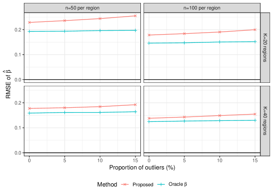
Figure 1: RMSE of $\widehat{\boldsymbol{\beta}}$, varying the number of outliers over 1000 replications.

Finally, to compare the performances in outlier detection, we used Matthews Correlation Coefficient (MCC), defined by

$${\rm MCC=\frac{TP\cdot TN-FP\cdot FN}{\sqrt{(TP+FP)(TP+FN)(TN+FP)(TN+FN)}}}.$$

Here, TP stands for true positive, where the detected outlier region is indeed an outlier; TN stands for true negative, where the labeled normal region is normal; FP stands for false positive, where the detected outlier region is actually normal; and FN stands for false negative, where the labelled normal region is actually an outlier. A higher value of MCC is preferred, where ${\rm MCC}=1$ indicates a perfect classifier and ${\rm MCC}=0$ indicates a random guess. We evaluated the MCC on the proposed, GLMM, Scan Statistic, and Oracle $\boldsymbol{\gamma}$. The MCCs are presented in Figure 2. The MCC of the Scan Statistic was around zero, even when $n$ and $K$ were increased, indicating that the Scan Statistic failed to detect multiple outlier regions. The MCC of the GLMM decreased when either the proportion of outlier or the $K$ increased. This is consistent with the literature suggesting that residual-based outlier detection may not operate well with multiple outliers. The MCC of the proposed method was comparable to its oracle counterpart, Oracle $\boldsymbol{\beta}$. It improved over increasing $K$ and stabilized over increasing proportion of outliers. In summary, our method showed promising performance in identifying outliers, especially when the proportion of outliers was increased.

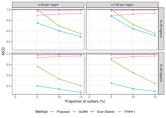
Figure 2: MCC, varying the number of outliers over 1000 replications.

5 Application to the PHINEX database

We considered census blockgroup as the geographic unit, and we excluded certain blockgroups with small sample sizes, following the guidelines of Behavioral Risk Factor Surveillance System [CDC, 2016]. The individual covariates $\boldsymbol{Z}_{ij}$ included sex, age as of 2012, race/ethnicity and insurance status, and the region-level covariates $\boldsymbol{X}_{i}$ included urbanicity and EHI. Age was categorized into 3 groups: 2–4 years, 5–9 years, and 10–14 years. Race and ethnicity were combined into a single covariate, and categorized into 4 groups: Hispanic, non-Hispanic white, non-Hispanic black, and non-Hispanic other. Patients with health service payor as commercial or Medicaid were included, where a few subjects with no insurance were excluded. Urbanicity, ranging from 1 to 11, was categorized into 3 groups: urban (1-4), suburban (5-8), or rural (9-11). We standardized EHI for numerical stability of the proposed algorithm.

The location $\boldsymbol{S}_{i}$ was defined by a vector of the longitude and latitude of the centroid of the $i$-th block group. We constructed $\rho_{i_{1},i_{2}}$ as the inverse of geodesic distances, $\rho_{i_{1},i_{2}}=1/d^{{\rm geo}}(\boldsymbol{S}_{i_{1}},\boldsymbol{S}_{i_{2}})$, where $d^{{\rm geo}}(\boldsymbol{S}_{i_{1}},\boldsymbol{S}_{i_{2}})$ denotes the greater circle distance between $\boldsymbol{S}_{i_{1}}$ and $\boldsymbol{S}_{i_{2}}$. For the $i_{1}$-th region, we retained the $L$ largest $\rho_{i_{1},i_{2}}$s and truncated the others at zero, where we treated $L$ as a tuning parameter. A grid search on $\lambda_{1}\in[2^{-1},2^{17}]$, $\lambda_{2}\in[2^{-5},2^{2}]$ and $L\in\{3,5,7\}$ was conducted to find the best combination of tuning parameters. The confidence interval of each parameter was constructed using bootstrap over 1000 replications.

Table 2: Fitted coefficients and confidence intervals (in parentheses) for covariate effects.

	Model
	Proposed	GLMM
Individual-level covariates
Sex (Base: Female)
$\sim$ Male	.235 (.144, .305)	.226 (.180, .271)
Age at 2012 (Base: Pre-school)
$\sim$ School-aged	.568 (.429, .657)	.562 (.491, .632)
$\sim$ Adolescent	.875 (.740, .967)	.869 (.802, .936)
Race/Ethnicity (Base: White, non-Hispanic)
$\sim$ Black, non-Hispanic	.437 (.313, .559)	.434 (.360, .508)
$\sim$ Other, non-Hispanic	.035 (-.133, .180)	.042 (-.068, .153)
$\sim$ Hispanic	.680 (.569, .787)	.667 (.606, .728)
Insurance status (Base: Commercial)
$\sim$ Medicaid	.522 (.428, .636)	.509 (.453, .565)
Community-level covariates
Urbanicity (Base: Urban)
$\sim$ Suburban	-.134 (-.305, -.034)	.037 (-.078, .152)
$\sim$ Rural	.125 (-.163, .302)	.237 (.070, .405)
Economic Hardship Index (standardized)	.120 (-.001, .147)	.143 (.095, .191)

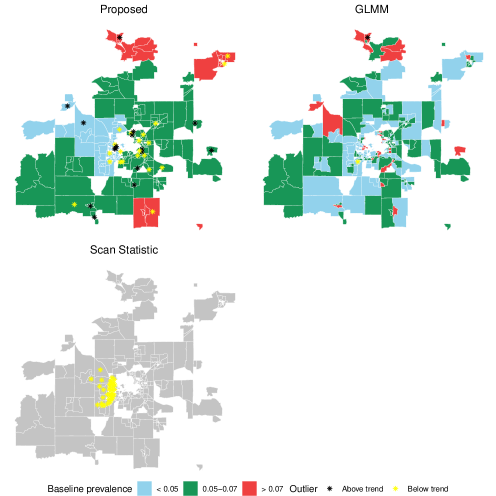
Figure 3: Estimated baseline prevalence rates and the identified outliers in childhood obesity surveillance. Each polygon represents a census blockgroup. Top-left: Result from the proposed method. Outliers are marked as black (yellow) as above the trend, $\widehat{\gamma}_{i}>0$ (below the trend, $\widehat{\gamma}_{i}<0$). Top-right: Result from the GLMM. Outliers are marked as black (yellow) as above the trend, $\widehat{b}_{i}>2.5\widehat{\sigma}$ (below the trend, $\widehat{b}_{i}<2.5\widehat{\sigma}$). Bottom-left: Discovered cluster by the Scan Statistic with the highest likelihood ratio, which was below the trend.

The estimated $\widehat{\boldsymbol{\alpha}}$s are summarized in Table 2. Overall, the proposed method had wider confidence intervals than the GLMM. This result was anticipated, given that our method had more parameters to estimate, which could lead to higher variabilities. The estimated coefficients from our model and the GLMM were comparable in general, except for the suburban effect. The obesity rate in females was lower compared to males, and younger children had lower obesity rates. Obesity rates in both non-Hispanic white and non-Hispanic other were lower than those in non-Hispanic black and Hispanic patients. The obesity prevalence was higher in subjects with Medicaid compared to those with commercial insurance. The EHI was positively associated with the estimated obesity rate.

The fitted baseline obesity rates are displayed in Figure 3, which appear to coincide with empirical knowledge of the greater Madison area. The lowest prevalence areas included the western portion of the Madison, Middleton, and Verona areas. It is known that these areas are recently developed and expanded, and include people who are generally younger and more socioeconomically advantaged compared to the surrounding areas. The intermediate prevalence areas, comprising the greater central and eastern Madison region, are more established, historic areas of the region, and are known to contain more stereotypical middle-class citizens. The highest prevalence areas are clearly the most geographically distant from the center of Madison, and are also all outside of Dane county, which contains Madison.

Table 3: The anonymized IDs of the outlier blockgroups, their sample sizes, crude obesity rates, fitted baseline obesity rates, adjusted obesity rates, and frequencies of detections over $B=1000$ bootstrap replications.

blockgroup	Unweighted	Crude	Fitted	Fitted	Frequency
ID	sample	obesity rate	baseline	adjusted	of
	size		obesity rate	obesity rate	detection
	($n_{i}$)	($\widehat{p}_{i}^{\rm crude}$)	($\widehat{p}_{i}^{\rm bsl}$)	($\widehat{p}_{i}^{\rm adj}$)	($\sum_{i}I(\widehat{\gamma}_{i}\neq 0)/B$)
Above the trend
7	60	.432	.097 (.061, .150)	.264 (.153, .351)	.701
23	91	.234	.048 (.042, .057)	.129 (.110, .167)	.483
24	93	.206	.048 (.042, .057)	.113 (.095, .128)	.515
25	104	.207	.048 (.042, .057)	.115 (.094, .139)	.496
83	96	.291	.058 (.047, .064)	.174 (.133, .179)	.689
85	91	.356	.058 (.047, .064)	.187 (.139, .196)	.895
100	62	.288	.058 (.047, .064)	.149 (.117, .155)	.763
102	53	.335	.058 (.047, .064)	.217 (.147, .246)	.579
124	66	.207	.058 (.047, .064)	.117 (.090, .136)	.535
200	93	.218	.058 (.047, .064)	.133 (.102, .151)	.474
212	100	.180	.048 (.042, .057)	.085 (.076, .094)	.634
244	71	.203	.053 (.044, .064)	.121 (.096, .135)	.446
245	94	.248	.053 (.044, .064)	.148 (.105, .184)	.573
252	68	.278	.056 (.046, .073)	.148 (.108, .179)	.706
254	82	.204	.058 (.048, .071)	.103 (.080, .111)	.698
264	74	.257	.048 (.042, .057)	.130 (.092, .157)	.726
Below the trend
22	110	.063	.048 (.042, .057)	.123 (.109, .151)	.363
32	221	.045	.048 (.042, .057)	.092 (.080, .101)	.079
35	146	.067	.048 (.042, .057)	.126 (.109, .151)	.300
70	67	.168	.058 (.047, .064)	.283 (.203, .292)	.269
73	109	.175	.058 (.047, .064)	.273 (.202, .279)	.136
82	259	.173	.058 (.047, .064)	.329 (.209, .342)	.106
94	134	.105	.058 (.047, .064)	.198 (.159, .210)	.383
115	68	.061	.058 (.047, .064)	.157 (.120, .161)	.468
118	192	.141	.058 (.047, .064)	.248 (.155, .253)	.062
125	81	.047	.058 (.047, .064)	.115 (.091, .115)	.277
127	295	.051	.058 (.047, .064)	.114 (.094, .121)	.195
128	125	.054	.058 (.047, .064)	.154 (.122, .175)	.698
136	466	.038	.048 (.042, .057)	.114 (.100, .132)	.684
153	469	.045	.048 (.042, .057)	.095 (.085, .103)	.047
159	202	.081	.058 (.047, .064)	.158 (.130, .176)	.345
168	139	.117	.056 (.046, .071)	.221 (.169, .247)	.418
186	66	.097	.058 (.047, .064)	.167 (.118, .184)	.204
229	133	.139	.077 (.048, .127)	.299 (.189, .395)	.599
235	61	.139	.077 (.048, .127)	.235 (.139, .312)	.365
246	210	.060	.053 (.044, .064)	.138 (.106, .158)	.283
262	90	.076	.081 (.050, .114)	.189 (.116, .237)	.459

The proposed method identified several outliers. Aberrant locations with obesity rates above the trend ($\widehat{\gamma}_{i}>0$) and below the trend ($\widehat{\gamma}_{i}<0$) were shown as black and yellow, respectively, in Figure 3. We identified 6% of blockgroups as outliers above the trend, and 8% as below the trend. Results are presented in Table 3, including:

• crude obesity rates, $\widehat{p}_{i}^{\rm crude}=\frac{1}{\sum_{j}w_{ij}I(R_{ij}=1)}\sum_{j}w_{ij}I(R_{ij}=1)Y_{ij}$;

• baseline obesity rates, $\widehat{p}_{i}^{\rm bsl}={\rm logit}^{-1}(\widehat{\beta}_{i})$;

• obesity rates adjusted for covariates and outliers,

  $$\widehat{p}_{i}^{\rm adj}=\widehat{\mathbb{E}}_{\gamma_{i}=0}(Y_{ij}|\boldsymbol{X}_{i})=\frac{1}{\sum_{j}w_{ij}I(R_{ij}=1)}\sum_{j=1}^{n_{i}}w_{ij}I(R_{ij}=1)\cdot{\rm logit}^{-1}\left(\boldsymbol{Z}_{ij}^{T}\widehat{\boldsymbol{\alpha}}_{1}+\boldsymbol{X}_{i}^{T}\widehat{\boldsymbol{\alpha}}_{2}+\widehat{\beta}_{i}\right),$$

and frequencies of detections over $B=1000$ bootstrap replications. We note that the outlier identification is relative to the fitted trend. For example, blockgroup 212 had an ordinary level of the estimated crude obesity rate (0.180). However, the crude rate was much higher than the fitted value of expected obesity prevalence (0.085). There existed unexplained information that could contribute to the elevated rate. Hence, it was declared as an outlier above the trend. The frequency of detection based on the bootstrap provides a glimpse of the uncertainty of aberrance. The outlier regions above the trend tended to have higher frequencies than those below the trend.

The localized outbreak from our model may enable comparative investigations at granular level. For example, what potential factors explain the outlier blockgroups that are significantly above or below the trend? Obesity prevalence is determined by the interplay of patient demographic characteristics, behaviors, and community environmental factors. Our model has accounted for only a subset of them. Thus outliers could represent communities with meaningfully different environments than expected (e.g. much better or worse than average access to grocery stores, parks, and recreational facilities), and/or it could represent community members with behaviors that are substantially different than expected (e.g. much greater or less physical activity, substantially better or worse dietary habits, etc.). Based on our results, healthcare professionals could look into the risk factors within the outlier and compare these factors with its adjacent blockgroups.

We also applied the GLMM and the Scan Statistic for comparison. As shown in Figure 3, the Scan Statistic identified midwestern Madison area as abnormal below trend, which appears to coincide with the lowest prevalence area identified by our method. However, it failed to inform outbreaks in obesity rates. These outbreaks could be captured by $\widehat{\boldsymbol{\gamma}}$ in our model. The GLMM does not smooth the obesity pattern over the state, which might be difficult to explain and investigate. Thus, the proposed method could provide more informative and interpretable results.

6 Concluding remarks

Motivated by childhood obesity surveillance using routinely collected EHR data, we developed a multilevel penalized logistic regression model. We incorporated the fusion and the nonconvex sparsity penalty in the likelihood function, which enabled us to conduct regional smoothing and outlier detection simultaneously. While in this paper we only considered spatial surveillance, we are interested in generalizing the method to longitudinal data setup that conducts spatiotemporal surveillance.

In our paper, we assume that BMI is MAR, which is not testable in observational data. The feasibility of MAR for EHRs data is an active area of research in recent years [Snyder et al., 2018]. In the future, we can develop sensitivity analysis techniques that investigate sensitivity of the results to uncontrolled confounding [Greenland, 2004].

Another future direction is to develop principled inferential procedures for the proposed work. We could potentially use ideas from significance testing and confidence regions for penalized procedures. For example, Hyun et al., [2016] developed a post-selection inference for generalized lasso applied to linear models. A general selective inference procedure for penalized likelihood has been developed for $\ell_{1}$ penalty [Taylor and Tibshirani, 2018].

Appendix A. Proof of Proposition 3.1

From the construction of the $\boldsymbol{\alpha}$- and $\boldsymbol{\gamma}$-steps, it is obvious that $\phi(\boldsymbol{\alpha}^{(t)},\boldsymbol{\beta}^{(t)},\boldsymbol{\gamma}^{(t)})\geq\phi(\boldsymbol{\alpha}^{(t+1)},\boldsymbol{\beta}^{(t)},\boldsymbol{\gamma}^{(t)})$ and $\phi(\boldsymbol{\alpha}^{(t+1)},\boldsymbol{\beta}^{(t+1)},\boldsymbol{\gamma}^{(t)})\geq\phi(\boldsymbol{\alpha}^{(t+1)},\boldsymbol{\beta}^{(t+1)},\boldsymbol{\gamma}^{(t+1)})$. To guarantee

$$\phi(\boldsymbol{\alpha}^{(t+1)},\boldsymbol{\beta}^{(t)},\boldsymbol{\gamma}^{(t)})\geq\phi(\boldsymbol{\alpha}^{(t+1)},\boldsymbol{\beta}^{(t+1)},\boldsymbol{\gamma}^{(t)}),$$

we verify a more general statement. Lemma 1 indicates that if an objective function $\psi(\cdot)$ consists of a smooth convex loss function $l(\cdot)$ plus a convex (and possibly non-differentiable) penalty $P(\cdot)$, one can descend $\psi$ by minimizing a surrogate function of $\psi$ in which the loss part $l$ is replaced by the local quadratic approximation of $l$.

Lemma 1.

Let $l(\boldsymbol{t})$ be a twicely-differentiable convex function and $P(\boldsymbol{t})$ be a convex function that is not necessarily differentiable. Define $\psi(\boldsymbol{t}):=l(\boldsymbol{t})+P(\boldsymbol{t})$. Let $\boldsymbol{t}^{0}$ be a fixed value in the domain of $\psi$. Define

$$\tilde{l}(\boldsymbol{t};\boldsymbol{t}^{0}):=l(\boldsymbol{t}^{0})+\nabla_{\boldsymbol{t}}l(\boldsymbol{t}^{0})^{T}(\boldsymbol{t}-\boldsymbol{t}^{0})+\frac{1}{2}(\boldsymbol{t}-\boldsymbol{t}^{0})^{T}\nabla_{\boldsymbol{t}\boldsymbol{t}}^{2}l(\boldsymbol{t}^{0})(\boldsymbol{t}-\boldsymbol{t}^{0}),~{}~{}~{}~{}\tilde{\psi}(\boldsymbol{t};\boldsymbol{t}^{0}):=\tilde{l}(\boldsymbol{t};\boldsymbol{t}^{0})+P(\boldsymbol{t}),$$

and $\boldsymbol{t}^{*}:=\operatornamewithlimits{argmin}_{\boldsymbol{t}}\tilde{\psi}(\boldsymbol{t};\boldsymbol{t}^{0})$. Consider

$$\boldsymbol{t}^{1}:=h^{*}\boldsymbol{t}^{*}+(1-h^{*})\boldsymbol{t}^{0},\mbox{~{}~{}where~{}}h^{*}:=\operatornamewithlimits{argmin}_{h\in[0,1]}\psi\left(h\boldsymbol{t}^{*}+(1-h)\boldsymbol{t}^{0}\right).$$

If $\boldsymbol{t}^{0}$ is not a minimizer of $\psi(\boldsymbol{t})$ (i.e., $\psi(\boldsymbol{t}^{0})<\psi(\boldsymbol{t}^{*})$), then such $h^{*}$ exists and $\psi(\boldsymbol{t}^{1})<\psi(\boldsymbol{t}^{0})$.

The proof is essentially the same as the proof of Proposition 1 in Lee et al., [2016]. They assumed $P(\boldsymbol{t})=\lambda\|\boldsymbol{t}\|_{1}$ for some $\lambda$, which can be easily extended to a general convex function $P(\cdot)$.

Proof.

Note that $\psi(\boldsymbol{t})$ and $\tilde{\psi}(\boldsymbol{t};\boldsymbol{t}^{0})$ have the same penalty function, and $\nabla_{\boldsymbol{t}}l(\boldsymbol{t})=\nabla_{\boldsymbol{t}}\tilde{l}(\boldsymbol{t}^{0};\boldsymbol{t}^{0})$. In addition, $\psi(\boldsymbol{t})$ and $\tilde{\psi}(\boldsymbol{t};\boldsymbol{t}^{0})$ have the same Karush-Kuhn-Tucker first-order optimality conditions at $\boldsymbol{t}=\boldsymbol{t}^{0}$. Then the assumption $\boldsymbol{t}^{0}\neq\operatornamewithlimits{argmin}_{\boldsymbol{t}}\psi(\boldsymbol{t})$ is equivalent to $\boldsymbol{t}^{0}\neq\operatornamewithlimits{argmin}_{\boldsymbol{t}}\tilde{\psi}(\boldsymbol{t};\boldsymbol{t}^{0})$. Consequently, $\tilde{\psi}(\boldsymbol{t}^{*};\boldsymbol{t}^{0})<\tilde{\psi}(\boldsymbol{t}^{0};\boldsymbol{t}^{0})$. Now let $h\in(0,1]$ and $\boldsymbol{t}^{h}=h\boldsymbol{t}^{*}+(1-h)\boldsymbol{t}^{0}$. The convexity of $\tilde{\psi}(\cdot;\boldsymbol{t}^{0})$ implies

$$\tilde{\psi}(\boldsymbol{t}^{h};\boldsymbol{t}^{0})\leq h\tilde{\psi}(\boldsymbol{t}^{*};\boldsymbol{t}^{0})+(1-h)\tilde{\psi}(\boldsymbol{t}^{0};\boldsymbol{t}^{0}),$$

which yields

$$\frac{\tilde{\psi}(\boldsymbol{t}^{h};\boldsymbol{t}^{0})-\tilde{\psi}(\boldsymbol{t}^{0};\boldsymbol{t}^{0})}{h}\leq\tilde{\psi}(\boldsymbol{t}^{*};\boldsymbol{t}^{0})-\tilde{\psi}(\boldsymbol{t}^{0};\boldsymbol{t}^{0})<0.$$

Furthermore,

$$\frac{\psi(\boldsymbol{t}^{h})-\psi(\boldsymbol{t}^{0})}{h}$$

$$= \frac{\tilde{\psi}(\boldsymbol{t}^{h};\boldsymbol{t}^{0})-\tilde{\psi}(\boldsymbol{t}^{0};\boldsymbol{t}^{0})}{h}-\frac{\tilde{l}(\boldsymbol{t}^{h};\boldsymbol{t}^{0})-\tilde{l}(\boldsymbol{t}^{0};\boldsymbol{t}^{0})}{h}+\frac{l(\boldsymbol{t}^{h})-l(\boldsymbol{t}^{0})}{h}$$

$$\leq \tilde{\psi}(\boldsymbol{t}^{*};\boldsymbol{t}^{0})-\tilde{\psi}(\boldsymbol{t}^{0};\boldsymbol{t}^{0})-\frac{\tilde{l}(\boldsymbol{t}^{h};\boldsymbol{t}^{0})-\tilde{l}(\boldsymbol{t}^{0};\boldsymbol{t}^{0})}{h}+\frac{l(\boldsymbol{t}^{h})-l(\boldsymbol{t}^{0})}{h}.$$

As $h\rightarrow 0^{+}$, $\tilde{\psi}(\boldsymbol{t}^{*};\boldsymbol{t}^{0})-\tilde{\psi}(\boldsymbol{t}^{0};\boldsymbol{t}^{0})-\{\tilde{l}(\boldsymbol{t}^{h};\boldsymbol{t}^{0})-\tilde{l}(\boldsymbol{t}^{0};\boldsymbol{t}^{0})\}/h$ converges to $-\nabla_{\boldsymbol{t}}\tilde{l}(\boldsymbol{t}^{0};\boldsymbol{t}^{0})+\nabla_{\boldsymbol{t}}l(\boldsymbol{t})$, which vanish to zero by the construction of $\tilde{l}$. Therefore, we have

$$\limsup_{h\rightarrow 0^{+}}\frac{\psi(\boldsymbol{t}^{h})-\psi(\boldsymbol{t}^{0})}{h}\leq\tilde{\psi}(\boldsymbol{t}^{*};\boldsymbol{t}^{0})-\tilde{\psi}(\boldsymbol{t}^{0};\boldsymbol{t}^{0})<0.$$

Therefore, there exists at least one $h\in(0,1]$ such that $\psi(\boldsymbol{t}^{h})<\psi(\boldsymbol{t}^{0})$. $\psi(\boldsymbol{t}^{1})<\psi(\boldsymbol{t}^{0})$ subsequently according to the construction of $\boldsymbol{t}^{1}$. ∎

Appendix B. Modified objective function adjusted for weights

Denote the final weight as $w_{ij}$ for $(ij)$-th subject. The modified objective function $\phi$ is defined by

$$\phi^{w}(\boldsymbol{\alpha},\boldsymbol{\beta},\boldsymbol{\gamma})=-{\rm loglik}^{w}(\boldsymbol{\alpha},\boldsymbol{\beta},\boldsymbol{\gamma})+P_{\lambda_{1}}(\boldsymbol{\beta})+Q_{\lambda_{2}}^{w}(\boldsymbol{\gamma}),$$ (7)

where

$${\rm loglik}^{w}(\boldsymbol{\alpha},\boldsymbol{\beta},\boldsymbol{\gamma}) = \frac{1}{w_{\cdot\cdot}}\sum_{i=1}^{K}\sum_{j=1}^{n_{i}}w_{ij}I(R_{ij}=1)\cdot\bigg{[}\log\{1+\exp({\boldsymbol{Z}}_{ij}^{T}\boldsymbol{\alpha}_{1}+{\boldsymbol{X}}_{i}^{T}\boldsymbol{\alpha}_{2}$$

$$\qquad+\beta_{i}+\gamma_{i})\}-Y_{ij}({\boldsymbol{Z}}_{ij}^{T}\boldsymbol{\alpha}_{1}+{\boldsymbol{X}}_{i}^{T}\boldsymbol{\alpha}_{2}+\beta_{i}+\gamma_{i})\bigg{]},$$

and

$$Q_{\lambda_{2}}^{w}(\boldsymbol{\gamma})=\frac{1}{w_{\cdot\cdot}}\sum_{i=1}^{K}w_{i\cdot}q_{\lambda_{2}}(\gamma_{i}),$$

with $w_{i\cdot}=\sum_{j}w_{ij}I(R_{ij}=1)$ and $w_{\cdot\cdot}=\sum_{i}\sum_{j}w_{ij}I(R_{ij}=1)$. The case of complete data can be understood as $w_{ij}=1$ and $R_{ij}=1$ for all $i$ and $j$. Algorithm 1 in Web Supplementary Materials describes the alternating minimization algorithm adjusted for the weight. The result of Proposition 1 remains the same as long as the dataset contains at least one obese and non-obese subject observed for all locations. The modified BIC reflecting the weight is

$${\rm BIC}^{w*}(\lambda_{1},\lambda_{2})=-2w_{\cdot\cdot}\cdot{\rm loglik}^{w}(\widehat{\boldsymbol{\alpha}},\widehat{\boldsymbol{\beta}},\widehat{\boldsymbol{\gamma}})+{\rm DF}\cdot\left(\log w_{\cdot\cdot}+1\right),$$

where ${\rm loglik}^{w}(\widehat{\boldsymbol{\alpha}},\widehat{\boldsymbol{\beta}},\widehat{\boldsymbol{\gamma}})$ is given in (7) and ${\rm DF}$ is given in (6) in Section 3.4.

Appendix C. Optimization algorithm

Algorithm 1 describes the proposed alternating minimization algorithm solving (7).

Algorithm 1 An alternating minimization algorithm for (7)

require: Arrays $\{Y_{ij}\}$, $\{\boldsymbol{Q}_{ij}\}$, $\{R_{ij}\}$ and $\{w_{ij}\}$, $i=1,\ldots,n_{i}$, $j=1,\ldots,K$, array $\{\rho_{i_{1},i_{2}}\}$, scalar $\lambda_{1}$ and scalar $\lambda_{2}$, tolerance level $\epsilon=10^{-6}$

initialize $\boldsymbol{\alpha}^{(0)}$, $\boldsymbol{\beta}^{(0)}$, $\boldsymbol{\gamma}^{(0)}$, $\phi^{(0)}=\phi(\boldsymbol{\alpha}^{(0)},\boldsymbol{\beta}^{(0)},\boldsymbol{\gamma}^{(0)})$

define $w_{i\cdot}\leftarrow\sum_{j}w_{ij}I(R_{ij}=1)$ and $w_{\cdot\cdot}\leftarrow\sum_{i}\sum_{j}w_{ij}I(R_{ij}=1)$

while  $\frac{|\phi^{(t+1)}-\phi^{(t)}|}{\max\{1,|\phi^{(t)}|\}}>\epsilon$ do

     

     (1. Updating $\boldsymbol{\alpha}$)

     1-1. $\mu_{ij}^{(t)}\leftarrow\beta_{i}^{(t)}+\gamma_{i}^{(t)}$ for $j=1,\ldots,n_{i}$, $i=1,\ldots,K$.

     1-2. Run a logistic regression, without intercept, for $N=\sum_{i=1}^{K}n_{i}$ individuals with response $\{Y_{ij}\}$, predictor $\{\boldsymbol{Q}_{ij}\}$, offset $\{\mu_{ij}^{(t)}\}$ and weight $\{w_{ij}\}$.

     1-3. Assign the results from Steps 1-1/1-2 to $\boldsymbol{\alpha}_{i}^{(t+1)}$.

     

     (2. Updating $\boldsymbol{\beta}$)

     2-1. $\theta_{ij}^{(t)}\leftarrow\boldsymbol{Q}_{ij}^{T}\boldsymbol{\alpha}^{(t+1)}+\gamma_{i}^{(t)}$ for $j=1,\ldots,n_{i}$, $i=1,\ldots,K$.

     2-2. $a_{i}^{(t)}\leftarrow\sum_{j=1}^{n_{i}}w_{ij}\left[\frac{\exp\left(\beta_{i}^{(t)}+\theta_{ij}^{(t)}\right)}{\left\{1+\exp\left(\beta_{i}^{(t)}+\theta_{ij}^{(t)}\right)\right\}^{2}}\right]$ for $i=1,\ldots,K$.

     2-3. $b_{i}^{(t)}\leftarrow\beta_{i}^{(t)}-\frac{1}{a_{i}^{(t)}}\sum_{j=1}^{n_{i}}w_{ij}\left[\frac{\exp\left(\beta_{i}^{(t)}+\theta_{ij}^{(t)}\right)}{1+\exp\left(\beta_{i}^{(t)}+\theta_{ij}^{(t)}\right)}-Y_{ij}\right]$ for $i=1,\ldots,K$.

     2-4. Solve

$$\tilde{\boldsymbol{\beta}}\leftarrow\operatornamewithlimits{argmin}_{\boldsymbol{\beta}\in\mathbb{R}^{K}}\left[\frac{1}{2w_{\cdot\cdot}}\sum_{i=1}^{K}a_{i}^{(t)}\left(\beta_{i}-b_{i}^{(t)}\right)^{2}+\lambda_{1}\sum_{i_{1}<i_{2}}\rho_{i_{1},i_{2}}|\beta_{i_{1}}-\beta_{i_{2}}|\right].$$

     2-5. If $\phi(\boldsymbol{\alpha}^{(t+1)},\tilde{\boldsymbol{\beta}},\boldsymbol{\gamma}^{(t)})\leq\phi(\boldsymbol{\alpha}^{(t+1)},\boldsymbol{\beta}^{(t)},\boldsymbol{\gamma}^{(t)})$, then $\boldsymbol{\beta}^{(t+1)}\leftarrow\tilde{\boldsymbol{\beta}}$. Otherwise, $\boldsymbol{\beta}^{(t+1)}\leftarrow\tilde{h}\tilde{\boldsymbol{\beta}}+(1-\tilde{h})\boldsymbol{\beta}^{(t)}$, where

$$\tilde{h}=\operatornamewithlimits{argmin}_{h\in[0,1]}\phi\left(\boldsymbol{\alpha}^{(t+1)},h\tilde{\boldsymbol{\beta}}+(1-h)\boldsymbol{\beta}^{(t)},\boldsymbol{\gamma}^{(t)}\right).$$

     

     (3. Updating $\boldsymbol{\gamma}$)

     3-1. $\nu_{ij}^{(t)}\leftarrow\boldsymbol{Q}_{ij}^{T}\boldsymbol{\alpha}^{(t+1)}+\beta_{i}^{(t+1)}$ for $j=1,\ldots,n_{i}$, $i=1,\ldots,K$.

     3-2. For $i=1,\ldots,K$ :

$$\gamma_{i}^{(t+1)}\leftarrow\operatornamewithlimits{argmin}_{\gamma}\left[\sum_{j=1}^{n_{i}}w_{ij}\left[\log\left\{1+\exp\left(\gamma+\nu_{ij}^{(t)}\right)\right\}-Y_{ij}\left(\gamma+\nu_{ij}^{(t)}\right)\right]+w_{i\cdot}q_{\lambda_{2}}(\gamma)\right].$$

     4. $\phi^{(t+1)}\leftarrow\phi(\boldsymbol{\alpha}^{(t+1)},\boldsymbol{\beta}^{(t+1)},\boldsymbol{\gamma}^{(t+1)})$

     

end while

return $(\boldsymbol{\alpha}^{(t+1)},\boldsymbol{\beta}^{(t+1)},\boldsymbol{\gamma}^{(t+1)})$

References

- Blondin et al., [2016] Blondin, K. J., Giles, C. M., Cradock, A. L., Gortmaker, S. L., and Long, M. W. (2016). US States’ childhood obesity surveillance practices and recommendations for improving them, 2014–2015. Preventing Chronic Disease, 13:160060.
- CDC, [2016] CDC (2016). Behavioral risk factor surveillance system, comparability of data BRFSS 2015 (Version #1—Revised: June 2016). Technical report.
- Davila-Payan et al., [2015] Davila-Payan, C., DeGuzman, M., Johnson, K., Serban, N., and Swann, J. (2015). Estimating prevalence of overweight or obese children and adolescents in small geographic areas using publicly available data. Preventing Chronic Disease, 12:E32.
- ESRI, [2012] ESRI (2012). Environmental Systems Research Institute (ESRI): tapestry segmentation reference guide. CA: Redlands.
- Farrington et al., [1996] Farrington, C. P., Andrews, N. J., Beale, A. D., and Catchpole, M. A. (1996). A statistical algorithm for the early detection of outbreaks of infectious disease. Journal of the Royal Statistical Society. Series A (Statistics in Society), 159(3):547.
- Flood et al., [2015] Flood, T. L., Zhao, Y.-Q., Tomayko, E. J., Tandias, A., Carrel, A. L., and Hanrahan, L. P. (2015). Electronic health records and community health surveillance of childhood obesity. American Journal of Preventive Medicine, 48(2):234–240.
- Friedman et al., [2013] Friedman, D. J., Parrish, R. G., and Ross, D. A. (2013). Electronic health records and US public health: Current realities and future promise. American Journal of Public Health, 103(9):1560–1567.
- Friedman et al., [2010] Friedman, J., Hastie, T., and Tibshirani, R. (2010). Regularization paths for generalized linear models via coordinate descent. Journal of Statistical Software, 33(1):1–22.
- Ghosh et al., [1999] Ghosh, M., Natarajan, K., Waller, L. A., and Kim, D. (1999). Hierarchical Bayes {GLMs} for the analysis of spatial data: An application to disease mapping. Journal of Statistical Planning and Inference, 75(2):305–318.
- Greenland, [2004] Greenland, S. (2004). The impact of prior distributions for uncontrolled confounding and response bias. Journal of the American Statistical Association, 98(461):47–54.
- Guilbert et al., [2012] Guilbert, T. W., Arndt, B., Temte, J., Adams, A., Buckingham, W., Tandias, A., Tomasallo, C., Anderson, H. A., and Hanrahan, L. P. (2012). The theory and application of UW ehealth-PHINEX, a clinical electronic health record-public health information exchange. WMJ, 111(3):124–33.
- Hoelscher et al., [2017] Hoelscher, D. M., Ranjit, N., and Pérez, A. (2017). Surveillance systems to track and evaluate obesity prevention efforts. Annual Review of Public Health, 38(1):187–214.
- Hyun et al., [2016] Hyun, S., G’sell, M., and Tibshirani, R. J. (2016). Exact post-selection inference for changepoint detection and other generalized lasso problems. arXiv preprint arXiv: 1606.03552.
- Jung, [2009] Jung, I. (2009). A generalized linear models approach to spatial scan statistics for covariate adjustment. Statistics in Medicine, 28(7):1131–1143.
- Kafadar and Stroup, [1992] Kafadar, K. and Stroup, D. F. (1992). Analysis of aberrations in public health surveillance data: Estimating variances on correlated samples. Statistics in Medicine, 11(12):1551–1568.
- Kim et al., [2009] Kim, S.-J., Koh, K., Boyd, S., and Gorinevsky, D. (2009). l1 Trend Filtering. SIAM Review, 51(2):339–360.
- Kulldorff, [1997] Kulldorff, M. (1997). A spatial scan statistic. Communications in Statistics - Theory and Methods, 26(6):1481–1496.
- Kulldorff and Nagarwalla, [1995] Kulldorff, M. and Nagarwalla, N. (1995). Spatial disease clusters: Detection and inference. Statistics in Medicine, 14(8):799–810.
- Lee, [2013] Lee, D. (2013). CARBayes: An R Package for Bayesian spatial modeling with conditional autoregressive priors. Journal of Statistical Software, 55(13):1–24.
- Lee et al., [2016] Lee, S., Kwon, S., and Kim, Y. (2016). A modified local quadratic approximation algorithm for penalized optimization problems. Computational Statistics and Data Analysis, 94:275–286.
- Little and Rubin, [2014] Little, R. J. and Rubin, D. B. (2014). Statistical Analysis with Missing Data. John Wiley & Sons.
- Longjohn et al., [2010] Longjohn, M., Sheon, A. R., Card-Higginson, P., Nader, P. R., and Mason, M. (2010). Learning from State surveillance of childhood obesity. Health Affairs, 29(3):463–472.
- Maiti et al., [2016] Maiti, T., Sinha, S., and Zhong, P.-S. (2016). Functional mixed effects model for small area estimation. Scandinavian Journal of Statistics, Theory and Applications, 43(3):886–903.
- Mass. Dep. Public Health, [2014] Mass. Dep. Public Health (2014). BMI screening guidelines for schools. Technical report, Mass. Dep. Public Health, Boston, MA.
- Mercer et al., [2015] Mercer, L. D., Wakefield, J., Pantazis, A., Lutambi, A. M., Masanja, H., and Clark, S. (2015). Space–time smoothing of complex survey data: Small area estimation for child mortality. The Annals of Applied Statistics, 9(4):1889–1905.
- Nathan and Adams, [1989] Nathan, R. P. and Adams, C. F. (1989). Four Perspectives on Urban Hardship. Political Science Quarterly, 104(3):483.
- Panczak et al., [2016] Panczak, R., Held, L., Moser, A., Jones, P. A., Rühli, F. J., and Staub, K. (2016). Finding big shots: Small-area mapping and spatial modeling of obesity among Swiss male conscripts. BMC Obesity, 3(1):1–12.
- Pascutto et al., [2000] Pascutto, C., Wakefield, J. C., Best, N. G., Richardson, S., Bernardinelli, L., Staines, A., and Elliott, P. (2000). Statistical issues in the analysis of disease mapping data. Statistics in Medicine, 19(17-18):2493–519.
- She and Owen, [2011] She, Y. and Owen, A. B. (2011). Outlier detection using nonconvex penalized regression. Journal of the American Statistical Association, 106(494):626–639.
- Snyder et al., [2018] Snyder, J. W., Bauer, C. R., Beaulieu-Jones, B. K., Pendergrass, S. A., Lavage, D. R., and Moore, J. H. (2018). Characterizing and managing missing structured data in electronic health records: Data analysis. JMIR Medical Informatics, 6(1):e11.
- Taylor and Tibshirani, [2018] Taylor, J. and Tibshirani, R. (2018). Post-selection inference for l1-penalized likelihood models. Canadian Journal of Statistics, 46(1):41–61.
- Tibshirani et al., [2005] Tibshirani, R., Saunders, M., Rosset, S., Zhu, J., and Knight, K. (2005). Sparsity and smoothness via the fused lasso. Journal of the Royal Statistical Society. Series B: Statistical Methodology, 67:91–108.
- Tibshirani and Taylor, [2011] Tibshirani, R. J. and Taylor, J. (2011). The solution path of the generalized lasso. The Annals of Statistics, 39(3):1335–1371.
- Ugarte et al., [2010] Ugarte, M. D., Goicoa, T., and Militino, A. F. (2010). Spatio-temporal modeling of mortality risks using penalized splines. Environmetrics, 21(3-4):270–289.
- Waller et al., [1997] Waller, L. A., Carlin, B. P., Xia, H., and Gelfand, A. E. (1997). Hierarchical spatio-temporal mapping of disease rates. Journal of the American Statistical Association, 92(438):607–617.
- Yu et al., [2015] Yu, D., Won, J.-H., Lee, T., Lim, J., and Yoon, S. (2015). High-dimensional fused lasso regression using majorization-minimization and parallel processing. Journal of Computational and Graphical Statistics, 24(1):121–153.
- Zhang et al., [2011] Zhang, Z., Zhang, L., Penman, A., and May, W. (2011). Using small-area estimation method to calculate county-level prevalence of obesity in Mississippi, 2007-2009. Preventing Chronic Disease, 8(4):A85.
- Zhao et al., [2011] Zhao, Y., Zeng, D., Herring, A. H., Ising, A., Waller, A., Richardson, D., and Kosorok, M. R. (2011). Detecting disease outbreaks using local spatiotemporal methods. Biometrics, 67(4):1508–1517.
- Zou et al., [2007] Zou, H., Hastie, T., and Tibshirani, R. (2007). On the “degrees of freedom” of the lasso. The Annals of Statistics, 35(5):2173–2192.