Data-Dependent Coresets for Compressing Neural Networks with Applications to Generalization Bounds

Cenk Baykal , Lucas Liebenwein†∗, Igor Gilitschenski, Dan Feldman , Daniela Rus Computer Science and Artificial Intelligence Laboratory, Massachusetts Institute of Technology,
emails: {baykal, lucasl, igilitschenski, rus}@mit.eduRobotics and Big Data Laboratory, University of Haifa, email: dannyf.post@gmail.comThese authors contributed equally to this work
Abstract

We present an efficient coresets-based neural network compression algorithm that sparsifies the parameters of a trained fully-connected neural network in a manner that provably approximates the network’s output. Our approach is based on an importance sampling scheme that judiciously defines a sampling distribution over the neural network parameters, and as a result, retains parameters of high importance while discarding redundant ones. We leverage a novel, empirical notion of sensitivity and extend traditional coreset constructions to the application of compressing parameters. Our theoretical analysis establishes guarantees on the size and accuracy of the resulting compressed network and gives rise to generalization bounds that may provide new insights into the generalization properties of neural networks. We demonstrate the practical effectiveness of our algorithm on a variety of neural network configurations and real-world data sets.

1 Introduction

Within the past decade, large-scale neural networks have demonstrated unprecedented empirical success in high-impact applications such as object classification, speech recognition, computer vision, and natural language processing. However, with the ever-increasing size of state-of-the-art neural networks, the resulting storage requirements and performance of these models are becoming increasingly prohibitive in terms of both time and space. Recently proposed architectures for neural networks, such as those in Krizhevsky et al. (2012); Long et al. (2015); Badrinarayanan et al. (2015), contain millions of parameters, rendering them prohibitive to deploy on platforms that are resource-constrained, e.g., embedded devices, mobile phones, or small scale robotic platforms.

In this work, we consider the problem of sparsifying the parameters of a trained fully-connected neural network in a principled way so that the output of the compressed neural network is approximately preserved. We introduce a neural network compression approach based on identifying and removing weighted edges with low relative importance via coresets, small weighted subsets of the original set that approximate the pertinent cost function. Our compression algorithm hinges on extensions of the traditional sensitivity-based coresets framework (Langberg & Schulman, 2010; Braverman et al., 2016), and to the best of our knowledge, is the first to apply coresets to parameter downsizing. In this regard, our work aims to simultaneously introduce a practical algorithm for compressing neural network parameters with provable guarantees and close the research gap in prior coresets work, which has predominantly focused on compressing input data points.

In particular, this paper contributes the following:

  1. 1.

    A coreset approach to compressing problem-specific parameters based on a novel, empirical notion of sensitivity that extends state-of-the-art coreset constructions.

  2. 2.

    An efficient neural network compression algorithm, CoreNet, based on our extended coreset approach that sparsifies the parameters via importance sampling of weighted edges.

  3. 3.

    Extensions of the CoreNet method, CoreNet+ and CoreNet++, that improve upon the edge sampling approach by additionally performing neuron pruning and amplification.

  4. 4.

    Analytical results establishing guarantees on the approximation accuracy, size, and generalization of the compressed neural network.

  5. 5.

    Evaluations on real-world data sets that demonstrate the practical effectiveness of our algorithm in compressing neural network parameters and validate our theoretical results.

2 Related Work

Our work builds upon the following prior work in coresets and compression approaches.

Coresets Coreset constructions were originally introduced in the context of computational geometry (Agarwal et al., 2005) and subsequently generalized for applications to other problems via an importance sampling-based, sensitivity framework (Langberg & Schulman, 2010; Braverman et al., 2016). Coresets have been used successfully to accelerate various machine learning algorithms such as k𝑘k-means clustering (Feldman & Langberg, 2011; Braverman et al., 2016), graphical model training (Molina et al., 2018), and logistic regression (Huggins et al., 2016) (see the surveys of Bachem et al. (2017) and Munteanu & Schwiegelshohn (2018) for a complete list). In contrast to prior work, we generate coresets for reducing the number of parameters – rather than data points – via a novel construction scheme based on an efficiently-computable notion of sensitivity.

Low-rank Approximations and Weight-sharing Denil et al. (2013) were among the first to empirically demonstrate the existence of significant parameter redundancy in deep neural networks. A predominant class of compression approaches consists of using low-rank matrix decompositions, such as Singular Value Decomposition (SVD) (Denton et al., 2014), to approximate the weight matrices with their low-rank counterparts. Similar works entail the use of low-rank tensor decomposition approaches applicable both during and after training (Jaderberg et al., 2014; Kim et al., 2015; Tai et al., 2015; Ioannou et al., 2015; Alvarez & Salzmann, 2017; Yu et al., 2017). Another class of approaches uses feature hashing and weight sharing (Weinberger et al., 2009; Shi et al., 2009; Chen et al., 2015b; a; Ullrich et al., 2017). Building upon the idea of weight-sharing, quantization (Gong et al., 2014; Wu et al., 2016; Zhou et al., 2017) or regular structure of weight matrices was used to reduce the effective number of parameters (Zhao et al., 2017; Sindhwani et al., 2015; Cheng et al., 2015; Choromanska et al., 2016; Wen et al., 2016). Despite their practical effectiveness in compressing neural networks, these works generally lack performance guarantees on the quality of their approximations and/or the size of the resulting compressed network.

Weight Pruning Similar to our proposed method, weight pruning (LeCun et al., 1990) hinges on the idea that only a few dominant weights within a layer are required to approximately preserve the output. Approaches of this flavor have been investigated by Lebedev & Lempitsky (2016); Dong et al. (2017), e.g., by embedding sparsity as a constraint (Iandola et al., 2016; Aghasi et al., 2017; Lin et al., 2017). Another related approach is that of Han et al. (2015), which considers a combination of weight pruning and weight sharing methods. Nevertheless, prior work in weight pruning lacks rigorous theoretical analysis of the effect that the discarded weights can have on the compressed network. To the best of our knowledge, our work is the first to introduce a practical, sampling-based weight pruning algorithm with provable guarantees.

Generalization The generalization properties of neural networks have been extensively investigated in various contexts (Dziugaite & Roy, 2017; Neyshabur et al., 2017a; Bartlett et al., 2017). However, as was pointed out by Neyshabur et al. (2017b), current approaches to obtaining non-vacuous generalization bounds do not fully or accurately capture the empirical success of state-of-the-art neural network architectures. Recently, Arora et al. (2018) and Zhou et al. (2018) highlighted the close connection between compressibility and generalization of neural networks. Arora et al. (2018) presented a compression method based on the Johnson-Lindenstrauss (JL) Lemma (Johnson & Lindenstrauss, 1984) and proved generalization bounds based on succinct reparameterizations of the original neural network. Building upon the work of Arora et al. (2018), we extend our theoretical compression results to establish novel generalization bounds for fully-connected neural networks. Unlike the method of Arora et al. (2018), which exhibits guarantees of the compressed network’s performance only on the set of training points, our method’s guarantees hold (probabilistically) for any random point drawn from the distribution. In addition, we establish that our method can ε𝜀\varepsilon-approximate the neural network output neuron-wise, which is stronger than the norm-based guarantee of Arora et al. (2018).

In contrast to prior work, this paper addresses the problem of compressing a fully-connected neural network while provably preserving the network’s output. Unlike previous theoretically-grounded compression approaches – which provide guarantees in terms of the normed difference –, our method provides the stronger entry-wise approximation guarantee, even for points outside of the available data set. As our empirical results show, ensuring that the output of the compressed network entry-wise approximates that of the original network is critical to retaining high classification accuracy. Overall, our compression approach remedies the shortcomings of prior approaches in that it (i) exhibits favorable theoretical properties, (ii) is computationally efficient, e.g., does not require retraining of the neural network, (iii) is easy to implement, and (iv) can be used in conjunction with other compression approaches – such as quantization or Huffman coding – to obtain further improved compression rates.

3 Problem Definition

3.1 Fully-Connected Neural Networks

A feedforward fully-connected neural network with L+𝐿subscriptL\in\mathbb{N}_{+} layers and parameters θ𝜃\theta defines a mapping fθ:𝒳𝒴:subscript𝑓𝜃𝒳𝒴f_{\theta}:\mathcal{X}\to\mathcal{Y} for a given input x𝒳d𝑥𝒳superscript𝑑x\in\mathcal{X}\subseteq\mathbb{R}^{d} to an output y𝒴k𝑦𝒴superscript𝑘y\in\mathcal{Y}\subseteq\mathbb{R}^{k} as follows. Let η+superscript𝜂subscript\eta^{\ell}\in\mathbb{N}_{+} denote the number of neurons in layer [L]delimited-[]𝐿\ell\in[L], where [L]={1,,L}delimited-[]𝐿1𝐿[L]=\{1,\ldots,L\} denotes the index set, and where η1=dsuperscript𝜂1𝑑\eta^{1}=d and ηL=ksuperscript𝜂𝐿𝑘\eta^{L}=k. Further, let η==2Lη𝜂superscriptsubscript2𝐿superscript𝜂\eta=\sum_{\ell=2}^{L}\eta^{\ell} and η=max{2,,L}ηsuperscript𝜂subscript2𝐿superscript𝜂\eta^{*}=\max_{\ell\in\left\{2,\ldots,L\right\}}\eta^{\ell}. For layers {2,,L}2𝐿\ell\in\left\{2,\ldots,L\right\}, let Wη×η1superscript𝑊superscriptsuperscript𝜂superscript𝜂1W^{\ell}\in\mathbb{R}^{\eta^{\ell}\times\eta^{\ell-1}} be the weight matrix for layer \ell with entries denoted by wijsuperscriptsubscript𝑤𝑖𝑗w_{ij}^{\ell}, rows denoted by wi1×η1superscriptsubscript𝑤𝑖superscript1superscript𝜂1w_{i}^{\ell}\in\mathbb{R}^{1\times\eta^{\ell-1}}, and θ=(W2,,WL)𝜃superscript𝑊2superscript𝑊𝐿\theta=(W^{2},\ldots,W^{L}). For notational simplicity, we assume that the bias is embedded in the weight matrix. Then for an input vector xd𝑥superscript𝑑x\in\mathbb{R}^{d}, let a1=xsuperscript𝑎1𝑥a^{1}=x and z=Wa1ηsuperscript𝑧superscript𝑊superscript𝑎1superscriptsuperscript𝜂z^{\ell}=W^{\ell}a^{\ell-1}\in\mathbb{R}^{\eta^{\ell}}, {2,,L}for-all2𝐿\forall\ell\in\left\{2,\ldots,L\right\}, where a1=ϕ(z1)η1superscript𝑎1italic-ϕsuperscript𝑧1superscriptsuperscript𝜂1a^{\ell-1}=\phi(z^{\ell-1})\in\mathbb{R}^{\eta^{\ell-1}} denotes the activation. We consider the activation function to be the Rectified Linear Unit (ReLU) function, i.e., ϕ()=max{,0}italic-ϕ0\phi(\cdot)=\max\{\cdot\,,0\} (entry-wise, if the input is a vector). The output of the network for an input x𝑥x is fθ(x)=zLsubscript𝑓𝜃𝑥superscript𝑧𝐿f_{\theta}(x)=z^{L}, and in particular, for classification tasks the prediction is argmaxi[k]fθ(x)i=argmaxi[k]ziL.subscript𝑖delimited-[]𝑘subscript𝑓𝜃subscript𝑥𝑖subscript𝑖delimited-[]𝑘subscriptsuperscript𝑧𝐿𝑖\operatorname*{\arg\!\max}_{i\in[k]}f_{\theta}(x)_{i}=\operatorname*{\arg\!\max}_{i\in[k]}z^{L}_{i}.

3.2 Neural Network Coreset Problem

Consider the setting where a neural network fθ()subscript𝑓𝜃f_{\theta}(\cdot) has been trained on a training set of independent and identically distributed (i.i.d.) samples from a joint distribution on 𝒳×𝒴𝒳𝒴\mathcal{X}\times\mathcal{Y}, yielding parameters θ=(W2,,WL)𝜃superscript𝑊2superscript𝑊𝐿\theta=(W^{2},\ldots,W^{L}). We further denote the input points of a validation data set as 𝒫={xi}i=1n𝒳𝒫superscriptsubscriptsubscript𝑥𝑖𝑖1𝑛𝒳\mathcal{P}=\left\{x_{i}\right\}_{i=1}^{n}\subseteq\mathcal{X} and the marginal distribution over the input space 𝒳𝒳\mathcal{X} as 𝒟𝒟{\mathcal{D}}. We define the size of the parameter tuple θ𝜃\theta, nnz(θ)nnz𝜃\mathrm{nnz}(\theta), to be the sum of the number of non-zero entries in the weight matrices W2,,WLsuperscript𝑊2superscript𝑊𝐿W^{2},\ldots,W^{L}.

For any given ε,δ(0,1)𝜀𝛿01\varepsilon,\delta\in(0,1), our overarching goal is to generate a reparameterization θ^^𝜃\hat{\theta}, yielding the neural network fθ^()subscript𝑓^𝜃f_{\hat{\theta}}(\cdot), using a randomized algorithm, such that nnz(θ^)nnz(θ)much-less-thannnz^𝜃nnz𝜃\mathrm{nnz}(\hat{\theta})\ll\mathrm{nnz}(\theta), and the neural network output fθ(x)subscript𝑓𝜃𝑥f_{\theta}(x), x𝒟similar-to𝑥𝒟x\sim{\mathcal{D}} can be approximated up to 1±εplus-or-minus1𝜀1\pm\varepsilon multiplicative error with probability greater than 1δ1𝛿1-\delta. We define the 1±εplus-or-minus1𝜀1\pm\varepsilon multiplicative error between two k𝑘k-dimensional vectors a,bk𝑎𝑏superscript𝑘a,b\in\mathbb{R}^{k} as the following entry-wise bound: a(1±ε)bai(1±ε)bii[k],𝑎plus-or-minus1𝜀𝑏subscript𝑎𝑖plus-or-minus1𝜀subscript𝑏𝑖for-all𝑖delimited-[]𝑘a\in(1\pm\varepsilon)b\,\Leftrightarrow\,a_{i}\in(1\pm\varepsilon)b_{i}\,\forall{i\in[k]}, and formalize the definition of an (ε,δ)𝜀𝛿(\varepsilon,\delta)-coreset as follows.

Definition 1 ((ε,δ)𝜀𝛿(\varepsilon,\delta)-coreset).

Given user-specified ε,δ(0,1)𝜀𝛿01\varepsilon,\delta\in(0,1), a set of parameters θ^=(W^2,,W^L)^𝜃superscript^𝑊2superscript^𝑊𝐿\hat{\theta}=(\hat{W}^{2},\ldots,\hat{W}^{L}) is an (ε,δ)𝜀𝛿(\varepsilon,\delta)-coreset for the network parameterized by θ𝜃\theta if for x𝒟similar-to𝑥𝒟x\sim{\mathcal{D}}, it holds that

θ^,x(fθ^(x)(1±ε)fθ(x))1δ,subscript^𝜃𝑥subscript𝑓^𝜃𝑥plus-or-minus1𝜀subscript𝑓𝜃𝑥1𝛿\operatorname*{\mathbb{P}}_{\hat{\theta},x}(f_{\hat{\theta}}(x)\in(1\pm\varepsilon)f_{\theta}(x))\geq 1-\delta,

where θ^,xsubscript^𝜃𝑥\operatorname*{\mathbb{P}}_{\hat{\theta},x} denotes a probability measure with respect to a random data point x𝑥x and the output θ^^𝜃\hat{\theta} generated by a randomized compression scheme.

4 Method

In this section, we introduce our neural network compression algorithm as depicted in Alg. 1. Our method is based on an important sampling-scheme that extends traditional sensitivity-based coreset constructions to the application of compressing parameters.

4.1 CoreNet

Our method (Alg. 1) hinges on the insight that a validation set of data points 𝒫i.i.d.𝒟n\mathcal{P}\stackrel{{\scriptstyle i.i.d.}}{{\sim}}{\mathcal{D}}^{n} can be used to approximate the relative importance, i.e., sensitivity, of each weighted edge with respect to the input data distribution 𝒟𝒟{\mathcal{D}}. For this purpose, we first pick a subsample of the data points SS𝒫SS𝒫\SS\subseteq\mathcal{P} of appropriate size (see Sec. 5 for details) and cache each neuron’s activation and compute a neuron-specific constant to be used to determine the required edge sampling complexity (Lines 2-6).

Algorithm 1 CoreNet

Input: ε,δ(0,1)𝜀𝛿01\varepsilon,\delta\in(0,1): error and failure probability, respectively; 𝒫𝒳𝒫𝒳\mathcal{P}\subseteq\mathcal{X}: a set of n𝑛n points from the input space 𝒳𝒳\mathcal{X} such that 𝒫i.i.d.𝒟n\mathcal{P}\stackrel{{\scriptstyle i.i.d.}}{{\sim}}{\mathcal{D}}^{n}; θ=(W2,,WL)𝜃superscript𝑊2superscript𝑊𝐿\theta=(W^{2},\ldots,W^{L}): parameters of the original uncompressed neural network. Output: θ^=(W^2,,W^L)^𝜃superscript^𝑊2superscript^𝑊𝐿\hat{\theta}=(\hat{W}^{2},\ldots,\hat{W}^{L}): sparsified parameter set such that fθ^()(1±ε)fθ()subscript𝑓^𝜃plus-or-minus1𝜀subscript𝑓𝜃f_{\hat{\theta}}(\cdot)\in(1\pm\varepsilon)f_{\theta}(\cdot) (see Sec. 5 for details).

1:εε2(L1)superscript𝜀𝜀2𝐿1\varepsilon^{\prime}\leftarrow\frac{\varepsilon}{2\,(L-1)};     ηmax{2,,L1}ηsuperscript𝜂subscript2𝐿1superscript𝜂\eta^{*}\leftarrow\max_{\ell\in\{2,\ldots,L-1\}}\eta^{\ell};     η=2Lη𝜂superscriptsubscript2𝐿superscript𝜂\eta\leftarrow\sum_{\ell=2}^{L}\eta^{\ell};     λlog(ηη)/2superscript𝜆𝜂superscript𝜂2\lambda^{*}\leftarrow\log(\eta\,\eta^{*})/2;
2:SSUniform sample (without replacement) of Klog(8ηη/δ)SSUniform sample (without replacement) of superscript𝐾8𝜂superscript𝜂𝛿\SS\leftarrow\text{Uniform sample (without replacement) of }\left\lceil K^{\prime}\log\left(8\,\eta\,\eta^{*}/\delta\right)\right\rceil points from 𝒫𝒫\mathcal{P};
3:a1(x)xxSSsuperscript𝑎1𝑥𝑥for-all𝑥SSa^{1}(x)\leftarrow x\quad\forall x\in\SS;
4:for xSS𝑥SSx\in\SS do
5:     for {2,,L}2𝐿\ell\in\left\{2,\ldots,L\right\} do
6:         a(x)ϕ(Wa1(x))superscript𝑎𝑥italic-ϕsuperscript𝑊superscript𝑎1𝑥a^{\ell}(x)\leftarrow\phi(W^{\ell}a^{\ell-1}(x));     Δi(x)k[η1]|wikak1(x)||k[η1]wikak1(x)|superscriptsubscriptΔ𝑖𝑥subscript𝑘delimited-[]superscript𝜂1superscriptsubscript𝑤𝑖𝑘superscriptsubscript𝑎𝑘1𝑥subscript𝑘delimited-[]superscript𝜂1superscriptsubscript𝑤𝑖𝑘superscriptsubscript𝑎𝑘1𝑥\Delta_{i}^{\ell}(x)\leftarrow\frac{\sum_{k\in[\eta^{\ell-1}]}|w_{ik}^{\ell}\,a_{k}^{\ell-1}({x})|}{\left|\sum_{k\in[\eta^{\ell-1}]}w_{ik}^{\ell}\,a_{k}^{\ell-1}({x})\right|};      
7:for {2,,L}2𝐿\ell\in\left\{2,\ldots,L\right\} do
8:     Δ^(1|SS|maxi[η]xSSΔi(x))+κ, where κ=2λ(1+2λlog(8ηη/δ))formulae-sequencesuperscript^Δ1SSsubscript𝑖delimited-[]superscript𝜂subscript𝑥SSsuperscriptsubscriptΔ𝑖𝑥𝜅 where 𝜅2subscript𝜆12subscript𝜆8𝜂superscript𝜂𝛿\hat{\Delta}^{\ell}\leftarrow\left(\frac{1}{|\SS|}\max_{i\in[\eta^{\ell}]}\,\sum_{x\in\SS}\Delta_{i}^{\ell}(x)\right)+\kappa,\,\text{ where }\,\kappa=\sqrt{2\lambda_{*}}\left(1+\sqrt{2\lambda_{*}}\log\left(8\,\eta\,\eta^{*}/\delta\right)\right);
9:     W^(0,,0)η×η1superscript^𝑊00superscriptsuperscript𝜂superscript𝜂1\hat{W}^{\ell}\leftarrow(\vec{0},\ldots,\vec{0})\in\mathbb{R}^{\eta^{\ell}\times\eta^{\ell-1}};     Δ^k=LΔ^ksuperscript^Δabsentsuperscriptsubscriptproduct𝑘𝐿superscript^Δ𝑘\hat{\Delta}^{\ell\rightarrow}\leftarrow\prod_{k=\ell}^{L}\hat{\Delta}^{k};     εεΔ^subscript𝜀superscript𝜀superscript^Δabsent\varepsilon_{\ell}\leftarrow\frac{\varepsilon^{\prime}}{\hat{\Delta}^{\ell\rightarrow}};
10:     for all i[η]𝑖delimited-[]superscript𝜂i\in[\eta^{\ell}] do
11:         𝒲+{j[η1]:wij>0}subscript𝒲conditional-set𝑗delimited-[]superscript𝜂1superscriptsubscript𝑤𝑖𝑗0\mathcal{W}_{+}\leftarrow\{j\in[\eta^{\ell-1}]:w_{ij}^{\ell}>0\};    𝒲{j[η1]:wij<0}subscript𝒲conditional-set𝑗delimited-[]superscript𝜂1superscriptsubscript𝑤𝑖𝑗0\mathcal{W}_{-}\leftarrow\{j\in[\eta^{\ell-1}]:w_{ij}^{\ell}<0\};
12:         w^i+Sparsify(𝒲+,wi,ε,δ,SS,a1)superscriptsubscript^𝑤𝑖limit-fromSparsifysubscript𝒲superscriptsubscript𝑤𝑖subscript𝜀𝛿SSsuperscript𝑎1{\hat{w}_{i}}^{\ell+}\leftarrow\textsc{Sparsify}(\mathcal{W}_{+},w_{i}^{\ell},\varepsilon_{\ell},\delta,\SS,a^{\ell-1});     w^iSparsify(𝒲,wi,ε,δ,SS,a1)superscriptsubscript^𝑤𝑖limit-fromSparsifysubscript𝒲superscriptsubscript𝑤𝑖subscript𝜀𝛿SSsuperscript𝑎1{\hat{w}_{i}}^{\ell-}\leftarrow\textsc{Sparsify}(\mathcal{W}_{-},-w_{i}^{\ell},\varepsilon_{\ell},\delta,\SS,a^{\ell-1});
13:         w^iw^i+w^isuperscriptsubscript^𝑤𝑖superscriptsubscript^𝑤𝑖limit-fromsuperscriptsubscript^𝑤𝑖limit-from{\hat{w}_{i}}^{\ell}\leftarrow{\hat{w}_{i}}^{\ell+}-{\hat{w}_{i}}^{\ell-};  W^iw^isubscriptsuperscript^𝑊𝑖superscriptsubscript^𝑤𝑖\hat{W}^{\ell}_{i\bullet}\leftarrow{\hat{w}_{i}}^{\ell};  \triangleright Consolidate the weights into the ithsuperscript𝑖thi^{\text{th}} row of W^superscript^𝑊\hat{W}^{\ell};      
14:return θ^=(W^2,,W^L)^𝜃superscript^𝑊2superscript^𝑊𝐿\hat{\theta}=(\hat{W}^{2},\ldots,\hat{W}^{L});
Algorithm 2 Sparsify(𝒲,w,ε,δ,SS,a())𝒲𝑤𝜀𝛿SS𝑎(\mathcal{W},w,\varepsilon,\delta,\SS,a(\cdot))

Input: 𝒲[η1]𝒲delimited-[]superscript𝜂1\mathcal{W}\subseteq[\eta^{\ell-1}]: index set; w1×η1𝑤superscript1superscript𝜂1w\in\mathbb{R}^{1\times\eta^{\ell-1}}: row vector corresponding to the weights incoming to node i[η]𝑖delimited-[]superscript𝜂i\in[\eta^{\ell}] in layer {2,,L}2𝐿\ell\in\left\{2,\ldots,L\right\}; ε,δ(0,1)𝜀𝛿01\varepsilon,\delta\in(0,1): error and failure probability, respectively; SS𝒫SS𝒫\SS\subseteq\mathcal{P}: subsample of the original point set; a()𝑎a(\cdot): cached activations of previous layer for all xSS𝑥SSx\in\SS.

Output: w^^𝑤{\hat{w}}: sparse weight vector.

1:for j𝒲𝑗𝒲j\in\mathcal{W} do
2:     sjmaxxSSwjaj(x)k𝒲wkak(x)subscript𝑠𝑗subscript𝑥SSsubscript𝑤𝑗subscript𝑎𝑗𝑥subscript𝑘𝒲subscript𝑤𝑘subscript𝑎𝑘𝑥s_{j}\leftarrow\max_{x\in\SS}\frac{w_{j}a_{j}(x)}{\sum_{k\in\mathcal{W}}w_{k}a_{k}(x)}; \triangleright Compute the sensitivity of each edge
3:Sj𝒲sj𝑆subscript𝑗𝒲subscript𝑠𝑗S\leftarrow\sum_{j\in\mathcal{W}}s_{j};
4:for j𝒲𝑗𝒲j\in\mathcal{W} do \triangleright Generate the importance sampling distribution over the incoming edges
5:     qjsjSsubscript𝑞𝑗subscript𝑠𝑗𝑆q_{j}\leftarrow\frac{s_{j}}{S};
6:m8SKlog(8η/δ)ε2𝑚8𝑆𝐾8𝜂𝛿superscript𝜀2m\leftarrow\left\lceil\frac{8\,S\,K\log({8\,\eta/\delta})}{{\varepsilon}^{2}}\right\rceil; \triangleright Compute the number of required samples
7:𝒞𝒞absent\mathcal{C}\leftarrow a multiset of m𝑚m samples from 𝒲𝒲\mathcal{W} where each j𝒲𝑗𝒲j\in\mathcal{W} is sampled with probability qjsubscript𝑞𝑗q_{j};
8:w^(0,,0)1×η1^𝑤00superscript1superscript𝜂1{\hat{w}}\leftarrow(0,\ldots,0)\in\mathbb{R}^{1\times\eta^{\ell-1}}; \triangleright Initialize the compressed weight vector
9:for j𝒞𝑗𝒞j\in\mathcal{C} do \triangleright Update the entries of the sparsified weight matrix according to the samples 𝒞𝒞\mathcal{C}
10:     w^jw^j+wjmqjsubscript^𝑤𝑗subscript^𝑤𝑗subscript𝑤𝑗𝑚subscript𝑞𝑗{\hat{w}_{j}}\leftarrow{\hat{w}_{j}}+\frac{w_{j}}{m\,q_{j}}; \triangleright Entries are reweighted by 1mqj1𝑚subscript𝑞𝑗\frac{1}{m\,q_{j}} to ensure unbiasedness of our estimator
11:return w^^𝑤{\hat{w}};

Subsequently, we apply our core sampling scheme to sparsify the set of incoming weighted edges to each neuron in all layers (Lines 7-13). For technical reasons (see Sec. 5), we perform the sparsification on the positive and negative weighted edges separately and then consolidate the results (Lines 11-13). By repeating this procedure for all neurons in every layer, we obtain a set θ^=(W^2,,W^L)^𝜃superscript^𝑊2superscript^𝑊𝐿\hat{\theta}=(\hat{W}^{2},\ldots,\hat{W}^{L}) of sparse weight matrices such that the output of each layer and the entire network is approximately preserved, i.e., W^a^1(x)Wa1(x)superscript^𝑊superscript^𝑎1𝑥superscript𝑊superscript𝑎1𝑥\hat{W}^{\ell}\hat{a}^{\ell-1}(x)\approx W^{\ell}a^{\ell-1}(x) and fθ^(x)fθ(x)subscript𝑓^𝜃𝑥subscript𝑓𝜃𝑥f_{\hat{\theta}}(x)\approx f_{\theta}(x), respectively111a^1(x)superscript^𝑎1𝑥\hat{a}^{\ell-1}(x) denotes the approximation from previous layers for an input x𝒟similar-to𝑥𝒟x\sim{\mathcal{D}}; see Sec. 5 for details..

4.2 Sparsifying Weights

The crux of our compression scheme lies in Alg. 2 (invoked twice on Line 12, Alg. 1) and in particular, in the importance sampling scheme used to select a small subset of edges of high importance. The cached activations are used to compute the sensitivity, i.e., relative importance, of each considered incoming edge j𝒲𝑗𝒲j\in\mathcal{W} to neuron i[η]𝑖delimited-[]superscript𝜂i\in[\eta^{\ell}], {2,,L}2𝐿\ell\in\left\{2,\ldots,L\right\} (Alg. 2, Lines 1-2). The relative importance of each edge j𝑗j is computed as the maximum (over xSS𝑥SSx\in\SS) ratio of the edge’s contribution to the sum of contributions of all edges. In other words, the sensitivity sjsubscript𝑠𝑗s_{j} of an edge j𝑗j captures the highest (relative) impact j𝑗j had on the output of neuron i[η]𝑖delimited-[]superscript𝜂i\in[\eta^{\ell}] in layer \ell across all xSS𝑥SSx\in\SS.

The sensitivities are then used to compute an importance sampling distribution over the incoming weighted edges (Lines 4-5). The intuition behind the importance sampling distribution is that if sjsubscript𝑠𝑗s_{j} is high, then edge j𝑗j is more likely to have a high impact on the output of neuron i𝑖i, therefore we should keep edge j𝑗j with a higher probability. m𝑚m edges are then sampled with replacement (Lines 6-7) and the sampled weights are then reweighed to ensure unbiasedness of our estimator (Lines 9-10).

4.3 Extensions: Neuron Pruning and Amplification

In this subsection we outline two improvements to our algorithm that that do not violate any of our theoretical properties and may improve compression rates in practical settings.

Neuron pruning (CoreNet+) Similar to removing redundant edges, we can use the empirical activations to gauge the importance of each neuron. In particular, if the maximum activation (over all evaluations xSS𝑥SSx\in\SS) of a neuron is equal to 0, then the neuron – along with all of the incoming and outgoing edges – can be pruned without significantly affecting the output with reasonable probability. This intuition can be made rigorous under the assumptions outlined in Sec. 5.

Amplification (CoreNet++) Coresets that provide stronger approximation guarantees can be constructed via amplification – the procedure of constructing multiple approximations (coresets) (w^i)1,,(w^i)τsubscriptsuperscriptsubscript^𝑤𝑖1subscriptsuperscriptsubscript^𝑤𝑖𝜏({\hat{w}_{i}}^{\ell})_{1},\ldots,({\hat{w}_{i}}^{\ell})_{\tau} over τ𝜏\tau trials, and picking the best one. To evaluate the quality of each approximation, a different subset 𝒯𝒫SS𝒯𝒫SS\mathcal{T}\subseteq\mathcal{P}\setminus\SS can be used to infer performance. In practice, amplification would entail constructing multiple approximations by executing Line 12 of Alg. 1 and picking the one that achieves the lowest relative error on 𝒯𝒯\mathcal{T}.

5 Analysis

In this section, we establish the theoretical guarantees of our neural network compression algorithm (Alg. 1). The full proofs of all the claims presented in this section can be found in the Appendix.

5.1 Preliminaries

Let x𝒟similar-to𝑥𝒟x\sim{\mathcal{D}} be a randomly drawn input point. We explicitly refer to the pre-activation and activation values at layer {2,,}2\ell\in\{2,\ldots,\ell\} with respect to the input xsupp(𝒟)𝑥supp𝒟x\in\mathrm{supp}({\mathcal{D}}) as z(x)superscript𝑧𝑥z^{\ell}(x) and a(x)superscript𝑎𝑥a^{\ell}(x), respectively. The values of z(x)superscript𝑧𝑥z^{\ell}(x) and a(x)superscript𝑎𝑥a^{\ell}(x) at each layer \ell will depend on whether or not we compressed the previous layers {2,,}superscript2\ell^{\prime}\in\{2,\ldots,\ell\}. To formalize this interdependency, we let z^(x)superscript^𝑧𝑥\hat{z}^{\ell}(x) and a^(x)superscript^𝑎𝑥\hat{a}^{\ell}(x) denote the respective quantities of layer \ell when we replace the weight matrices W2,,Wsuperscript𝑊2superscript𝑊W^{2},\ldots,W^{\ell} in layers 2,,22,\ldots,\ell by W^2,,W^superscript^𝑊2superscript^𝑊\hat{W}^{2},\ldots,\hat{W}^{\ell}, respectively.

For the remainder of this section (Sec. 5) we let {2,,L}2𝐿\ell\in\left\{2,\ldots,L\right\} be an arbitrary layer and let i[η]𝑖delimited-[]superscript𝜂i\in[\eta^{\ell}] be an arbitrary neuron in layer \ell. For purposes of clarity and readability, we will omit the the variable denoting the layer {2,,L}2𝐿\ell\in\left\{2,\ldots,L\right\}, the neuron i[η]𝑖delimited-[]superscript𝜂i\in[\eta^{\ell}], and the incoming edge index j[η1]𝑗delimited-[]superscript𝜂1j\in[\eta^{\ell-1}], whenever they are clear from the context. For example, when referring to the intermediate value of a neuron i[η]𝑖delimited-[]superscript𝜂i\in[\eta^{\ell}] in layer {2,,L}2𝐿\ell\in\left\{2,\ldots,L\right\}, zi(x)=wi,a^1(x)superscriptsubscript𝑧𝑖𝑥superscriptsubscript𝑤𝑖superscript^𝑎1𝑥z_{i}^{\ell}(x)=\langle w_{i}^{\ell},\hat{a}^{\ell-1}(x)\rangle\in\mathbb{R} with respect to a point x𝑥x, we will simply write z(x)=w,a(x)𝑧𝑥𝑤𝑎𝑥z(x)=\langle w,a(x)\rangle\in\mathbb{R}, where w:=wi1×η1assign𝑤superscriptsubscript𝑤𝑖superscript1superscript𝜂1w:=w_{i}^{\ell}\in\mathbb{R}^{1\times\eta^{\ell-1}} and a(x):=a1(x)η1×1assign𝑎𝑥superscript𝑎1𝑥superscriptsuperscript𝜂11a(x):=a^{\ell-1}(x)\in\mathbb{R}^{\eta^{\ell-1}\times 1}. Under this notation, the weight of an incoming edge j𝑗j is denoted by wjsubscript𝑤𝑗w_{j}\in\mathbb{R}.

5.2 Importance Sampling Bounds for Positive Weights

In this subsection, we establish approximation guarantees under the assumption that the weights are positive. Moreover, we will also assume that the input, i.e., the activation from the previous layer, is non-negative (entry-wise). The subsequent subsection will then relax these assumptions to conclude that a neuron’s value can be approximated well even when the weights and activations are not all positive and non-negative, respectively. Let 𝒲={j[η1]:wj>0}[η1]𝒲conditional-set𝑗delimited-[]superscript𝜂1subscript𝑤𝑗0delimited-[]superscript𝜂1\mathcal{W}=\{j\in[\eta^{\ell-1}]:w_{j}>0\}\subseteq[\eta^{\ell-1}] be the set of indices of incoming edges with strictly positive weights. To sample the incoming edges to a neuron, we quantify the relative importance of each edge as follows.

Definition 2 (Relative Importance).

The importance of an incoming edge j𝒲𝑗𝒲j\in\mathcal{W} with respect to an input xsupp(𝒟)𝑥supp𝒟x\in\mathrm{supp}({\mathcal{D}}) is given by the function gj(x)subscript𝑔𝑗𝑥g_{j}(x), where gj(x)=wjaj(x)k𝒲wkak(x)j𝒲.subscript𝑔𝑗𝑥subscript𝑤𝑗subscript𝑎𝑗𝑥subscript𝑘𝒲subscript𝑤𝑘subscript𝑎𝑘𝑥for-all𝑗𝒲g_{j}(x)=\frac{w_{j}\,a_{j}(x)}{\sum_{k\in\mathcal{W}}w_{k}\,a_{k}(x)}\quad\forall{j\in\mathcal{W}}.

Note that gj(x)subscript𝑔𝑗𝑥g_{j}(x) is a function of the random variable x𝒟similar-to𝑥𝒟x\sim{\mathcal{D}}. We now present our first assumption that pertains to the Cumulative Distribution Function (CDF) of the relative importance random variable.

Assumption 1.

There exist universal constants K,K>0𝐾superscript𝐾0K,K^{\prime}>0 such that for all j𝒲𝑗𝒲j\in\mathcal{W}, the CDF of the random variable gj(x)subscript𝑔𝑗𝑥g_{j}(x) for x𝒟similar-to𝑥𝒟x\sim{\mathcal{D}}, denoted by Fj()subscript𝐹𝑗F_{j}\left(\cdot\right), satisfies

Fj(Mj/K)exp(1/K),subscript𝐹𝑗subscript𝑀𝑗𝐾1superscript𝐾F_{j}\left(\nicefrac{{M_{j}}}{{K}}\right)\leq\exp\left(-\nicefrac{{1}}{{K^{\prime}}}\right),

where Mj=min{y[0,1]:Fj(y)=1}subscript𝑀𝑗:𝑦01subscript𝐹𝑗𝑦1M_{j}=\min\{y\in[0,1]:F_{j}\left(y\right)=1\}.

Assumption 1 is a technical assumption on the ratio of the weighted activations that will enable us to rule out pathological problem instances where the relative importance of each edge cannot be well-approximated using a small number of data points SS𝒫SS𝒫\SS\subseteq\mathcal{P}. Henceforth, we consider a uniformly drawn (without replacement) subsample SS𝒫SS𝒫\SS\subseteq\mathcal{P} as in Line 2 of Alg. 1, where |SS|=Klog(8ηη/δ)SSsuperscript𝐾8𝜂superscript𝜂𝛿\left|\SS\right|=\left\lceil K^{\prime}\log\left(8\,\eta\,\eta^{*}/\delta\right)\right\rceil, and define the sensitivity of an edge as follows.

Definition 3 (Empirical Sensitivity).

Let SS𝒫SS𝒫\SS\subseteq\mathcal{P} be a subset of distinct points from 𝒫i.i.d.𝒟n\mathcal{P}\stackrel{{\scriptstyle i.i.d.}}{{\sim}}{\mathcal{D}}^{n}.Then, the sensitivity over positive edges j𝒲𝑗𝒲j\in\mathcal{W} directed to a neuron is defined as sj=maxxSSgj(x).subscript𝑠𝑗subscript𝑥SSsubscript𝑔𝑗𝑥s_{j}\,=\,\max_{x\in\SS}g_{j}(x).

Our first lemma establishes a core result that relates the weighted sum with respect to the sparse row vector w^^𝑤{\hat{w}}, k𝒲w^ka^k(x)subscript𝑘𝒲subscript^𝑤𝑘subscript^𝑎𝑘𝑥\sum_{k\in\mathcal{W}}{\hat{w}}_{k}\,\hat{a}_{k}(x), to the value of the of the weighted sum with respect to the ground-truth row vector w𝑤w, k𝒲wka^k(x)subscript𝑘𝒲subscript𝑤𝑘subscript^𝑎𝑘𝑥\sum_{k\in\mathcal{W}}w_{k}\,\hat{a}_{k}(x). We remark that there is randomness with respect to the randomly generated row vector w^isuperscriptsubscript^𝑤𝑖{\hat{w}_{i}}^{\ell}, a randomly drawn input x𝒟similar-to𝑥𝒟x\sim{\mathcal{D}}, and the function a^()=a^1()^𝑎superscript^𝑎1\hat{a}(\cdot)=\hat{a}^{\ell-1}(\cdot) defined by the randomly generated matrices W^2,,W^1superscript^𝑊2superscript^𝑊1\hat{W}^{2},\ldots,\hat{W}^{\ell-1} in the previous layers. Unless otherwise stated, we will henceforth use the shorthand notation ()\operatorname*{\mathbb{P}}(\cdot) to denote w^,x,a^1()subscriptsuperscript^𝑤𝑥superscript^𝑎1\operatorname*{\mathbb{P}}_{{\hat{w}}^{\ell},\,x,\,\hat{a}^{\ell-1}}(\cdot). Moreover, for ease of presentation, we will first condition on the event 1/2subscript12\mathcal{E}_{\nicefrac{{1}}{{2}}} that a^(x)(1±1/2)a(x)^𝑎𝑥plus-or-minus112𝑎𝑥\hat{a}(x)\in(1\pm\nicefrac{{1}}{{2}})a(x) holds. This conditioning will simplify the preliminary analysis and will be removed in our subsequent results.

Lemma 1 (Positive-Weights Sparsification).

Let ε,δ(0,1)𝜀𝛿01\varepsilon,\delta\in(0,1), and x𝒟similar-to𝑥𝒟x\sim{\mathcal{D}}. Sparsify(𝒲,w,ε,δ,SS,a())𝒲𝑤𝜀𝛿SS𝑎(\mathcal{W},w,\varepsilon,\delta,\SS,a(\cdot)) generates a row vector w^^𝑤{\hat{w}} such that

(k𝒲w^ka^k(x)(1±ε)k𝒲wka^k(x)1/2)subscript𝑘𝒲subscript^𝑤𝑘subscript^𝑎𝑘𝑥conditionalplus-or-minus1𝜀subscript𝑘𝒲subscript𝑤𝑘subscript^𝑎𝑘𝑥subscript12\displaystyle\operatorname*{\mathbb{P}}\left(\sum_{k\in\mathcal{W}}{\hat{w}}_{k}\,\hat{a}_{k}(x)\notin(1\pm\varepsilon)\sum_{k\in\mathcal{W}}w_{k}\,\hat{a}_{k}(x)\,\mid\,\mathcal{E}_{\nicefrac{{1}}{{2}}}\right) 3δ8ηabsent3𝛿8𝜂\displaystyle\leq\frac{3\delta}{8\eta}

where nnz(w^)8SKlog(8η/δ)ε2,nnz^𝑤8𝑆𝐾8𝜂𝛿superscript𝜀2\mathrm{nnz}({\hat{w}})\leq\left\lceil\frac{8\,S\,K\log({8\,\eta/\delta})}{{\varepsilon}^{2}}\right\rceil, and S=j𝒲sj𝑆subscript𝑗𝒲subscript𝑠𝑗S=\sum_{j\in\mathcal{W}}s_{j}.

5.3 Importance Sampling Bounds

We now relax the requirement that the weights are strictly positive and instead consider the following index sets that partition the weighted edges: 𝒲+={j[η1]:wj>0}subscript𝒲conditional-set𝑗delimited-[]superscript𝜂1subscript𝑤𝑗0\mathcal{W}_{+}=\{j\in[\eta^{\ell-1}]:w_{j}>0\} and 𝒲={j[η1]:wj<0}subscript𝒲conditional-set𝑗delimited-[]superscript𝜂1subscript𝑤𝑗0\mathcal{W}_{-}=\{j\in[\eta^{\ell-1}]:w_{j}<0\}. We still assume that the incoming activations from the previous layers are positive (this assumption can be relaxed as discussed in Appendix A.2.4). We define Δi(x)superscriptsubscriptΔ𝑖𝑥\Delta_{i}^{\ell}(x) for a point x𝒟similar-to𝑥𝒟x\sim{\mathcal{D}} and neuron i[η]𝑖delimited-[]superscript𝜂i\in[\eta^{\ell}] as Δi(x)=k[η1]|wikak1(x)||k[η1]wikak1(x)|.superscriptsubscriptΔ𝑖𝑥subscript𝑘delimited-[]superscript𝜂1superscriptsubscript𝑤𝑖𝑘superscriptsubscript𝑎𝑘1𝑥subscript𝑘delimited-[]superscript𝜂1superscriptsubscript𝑤𝑖𝑘superscriptsubscript𝑎𝑘1𝑥\Delta_{i}^{\ell}(x)=\frac{\sum_{k\in[\eta^{\ell-1}]}|w_{ik}^{\ell}\,a_{k}^{\ell-1}({x})|}{\left|\sum_{k\in[\eta^{\ell-1}]}w_{ik}^{\ell}\,a_{k}^{\ell-1}({x})\right|}. The following assumption serves a similar purpose as does Assumption 1 in that it enables us to approximate the random variable Δi(x)superscriptsubscriptΔ𝑖𝑥\Delta_{i}^{\ell}(x) via an empirical estimate over a small-sized sample of data points SS𝒫SS𝒫\SS\subseteq\mathcal{P}.

Assumption 2 (Subexponentiality of Δi(x)superscriptsubscriptΔ𝑖𝑥{\Delta_{i}^{\ell}(x)}).

There exists a universal constant λ>0𝜆0\lambda>0, λ<K/2𝜆superscript𝐾2\lambda<K^{\prime}/2222Where Ksuperscript𝐾K^{\prime} is as defined in Assumption 1 such that for any layer {2,,L}2𝐿\ell\in\left\{2,\ldots,L\right\} and neuron i[η]𝑖delimited-[]superscript𝜂i\in[\eta^{\ell}], the centered random variable Δ=Δi(x)𝔼x𝒟[Δi(x)]ΔsuperscriptsubscriptΔ𝑖𝑥subscript𝔼similar-to𝑥𝒟superscriptsubscriptΔ𝑖𝑥\Delta=\Delta_{i}^{\ell}(x)-\operatorname*{\mathbb{E}\,}_{x\sim{\mathcal{D}}}[\Delta_{i}^{\ell}(x)] is subexponential (Vershynin, 2016) with parameter λ𝜆\lambda, i.e., 𝔼[exp(sΔ)]exp(s2λ2)|s|1λ𝔼𝑠Δsuperscript𝑠2superscript𝜆2for-all𝑠1𝜆\operatorname*{\mathbb{E}\,}[\exp\left(s\Delta\right)]\leq\exp(s^{2}\lambda^{2})\quad\forall{|s|\leq\frac{1}{\lambda}}.

For ε(0,1)𝜀01\varepsilon\in(0,1) and {2,,L}2𝐿\ell\in\left\{2,\ldots,L\right\}, we let ε=ε2(L1)superscript𝜀𝜀2𝐿1\varepsilon^{\prime}=\frac{\varepsilon}{2\,(L-1)} and define ε=εΔ^=ε2(L1)k=LΔ^k,subscript𝜀superscript𝜀superscript^Δabsent𝜀2𝐿1superscriptsubscriptproduct𝑘𝐿superscript^Δ𝑘\varepsilon_{\ell}=\frac{\varepsilon^{\prime}}{\hat{\Delta}^{\ell\rightarrow}}=\frac{\varepsilon}{2\,(L-1)\prod_{k=\ell}^{L}\hat{\Delta}^{k}}, where Δ^=(1|SS|maxi[η]xSSΔi(x))+κsuperscript^Δ1SSsubscript𝑖delimited-[]superscript𝜂subscriptsuperscript𝑥SSsuperscriptsubscriptΔ𝑖superscript𝑥𝜅\hat{\Delta}^{\ell}=\left(\frac{1}{|\SS|}\max_{i\in[\eta^{\ell}]}\,\sum_{x^{\prime}\in\SS}\Delta_{i}^{\ell}(x^{\prime})\right)+\kappa. To formalize the interlayer dependencies, for each i[η]𝑖delimited-[]superscript𝜂i\in[\eta^{\ell}] we let isubscriptsuperscript𝑖\mathcal{E}^{\ell}_{i} denote the (desirable) event that z^i(x)(1±2(1)ε+1)zi(x)superscriptsubscript^𝑧𝑖𝑥plus-or-minus121subscript𝜀1subscriptsuperscript𝑧𝑖𝑥\hat{z}_{i}^{\ell}(x)\in\left(1\pm 2\,(\ell-1)\,\varepsilon_{\ell+1}\right)z^{\ell}_{i}(x) holds, and let =i[η]isuperscriptsubscript𝑖delimited-[]superscript𝜂superscriptsubscript𝑖\mathcal{E}^{\ell}=\cap_{i\in[\eta^{\ell}]}\,\mathcal{E}_{i}^{\ell} be the intersection over the events corresponding to each neuron in layer \ell.

Lemma 2 (Conditional Neuron Value Approximation).

Let ε,δ(0,1)𝜀𝛿01\varepsilon,\delta\in(0,1), {2,,L}2𝐿\ell\in\left\{2,\ldots,L\right\}, i[η]𝑖delimited-[]superscript𝜂i\in[\eta^{\ell}], and x𝒟similar-to𝑥𝒟x\sim{\mathcal{D}}. CoreNet generates a row vector w^i=w^i+w^i1×η1superscriptsubscript^𝑤𝑖superscriptsubscript^𝑤𝑖limit-fromsuperscriptsubscript^𝑤𝑖limit-fromsuperscript1superscript𝜂1{\hat{w}_{i}}^{\ell}={\hat{w}_{i}}^{\ell+}-{\hat{w}_{i}}^{\ell-}\in\mathbb{R}^{1\times\eta^{\ell-1}} such that

(i1)=(z^i(x)(1±2(1)ε+1)zi(x)1)1δ/η,conditionalsuperscriptsubscript𝑖superscript1superscriptsubscript^𝑧𝑖𝑥conditionalplus-or-minus121subscript𝜀1superscriptsubscript𝑧𝑖𝑥superscript11𝛿𝜂\displaystyle\operatorname*{\mathbb{P}}\big{(}\,\mathcal{E}_{i}^{\ell}\,\,\mid\,\mathcal{E}^{\ell-1}\big{)}=\operatorname*{\mathbb{P}}\left(\hat{z}_{i}^{\ell}(x)\in\left(1\pm 2\,(\ell-1)\,\varepsilon_{\ell+1}\right)z_{i}^{\ell}(x)\,\mid\,\mathcal{E}^{\ell-1}\right)\geq 1-\nicefrac{{\delta}}{{\eta}}, (1)

where ε=εΔ^subscript𝜀superscript𝜀superscript^Δabsent\varepsilon_{\ell}=\frac{\varepsilon^{\prime}}{\hat{\Delta}^{\ell\rightarrow}} and nnz(w^i)8SKlog(8η/δ)ε2+1,nnzsuperscriptsubscript^𝑤𝑖8𝑆𝐾8𝜂𝛿superscriptsubscript𝜀21\mathrm{nnz}({\hat{w}_{i}}^{\ell})\leq\left\lceil\frac{8\,S\,K\log({8\,\eta/\delta})}{{\varepsilon_{\ell}}^{2}}\right\rceil+1, where S=j𝒲+sj+j𝒲sj𝑆subscript𝑗subscript𝒲subscript𝑠𝑗subscript𝑗subscript𝒲subscript𝑠𝑗S=\sum_{j\in\mathcal{W}_{+}}s_{j}+\sum_{j\in\mathcal{W}_{-}}s_{j}.

The following core result establishes unconditional layer-wise approximation guarantees and culminates in our main compression theorem.

Lemma 3 (Layer-wise Approximation).

Let ε,δ(0,1)𝜀𝛿01\varepsilon,\delta\in(0,1), {2,,L}2𝐿\ell\in\left\{2,\ldots,L\right\}, and x𝒟similar-to𝑥𝒟x\sim{\mathcal{D}}. CoreNet generates a sparse weight matrix W^η×η1superscript^𝑊superscriptsuperscript𝜂superscript𝜂1\hat{W}^{\ell}\in{\mathbb{R}}^{\eta^{\ell}\times\eta^{\ell-1}} such that, for z^(x)=W^a^(x)superscript^𝑧𝑥superscript^𝑊superscript^𝑎𝑥\hat{z}^{\ell}(x)=\hat{W}^{\ell}\hat{a}^{\ell}(x),

(W^2,,W^),x()=(W^2,,W^),x(z^(x)(1±2(1)ε+1)z(x))1δ=2ηη.subscriptsuperscript^𝑊2superscript^𝑊𝑥superscriptsubscriptsuperscript^𝑊2superscript^𝑊𝑥superscript^𝑧𝑥plus-or-minus121subscript𝜀1superscript𝑧𝑥1𝛿superscriptsubscriptsuperscript2superscript𝜂superscript𝜂\operatorname*{\mathbb{P}}_{(\hat{W}^{2},\ldots,\hat{W}^{\ell}),\,x}(\mathcal{E}^{\ell})=\operatorname*{\mathbb{P}}_{(\hat{W}^{2},\ldots,\hat{W}^{\ell}),\,x}\left(\hat{z}^{\ell}(x)\in\left(1\pm 2\,(\ell-1)\,\varepsilon_{\ell+1}\right)z^{\ell}(x)\right)\geq 1-\frac{\delta\,\sum_{\ell^{\prime}=2}^{\ell}\eta^{\ell^{\prime}}}{\eta}.
Theorem 4 (Network Compression).

For ε,δ(0,1)𝜀𝛿01\varepsilon,\delta\in(0,1), Algorithm 1 generates a set of parameters θ^=(W^2,,W^L)^𝜃superscript^𝑊2superscript^𝑊𝐿\hat{\theta}=(\hat{W}^{2},\ldots,\hat{W}^{L}) of size

nnz(θ^)nnz^𝜃\displaystyle\mathrm{nnz}(\hat{\theta}) =2Li=1η(32(L1)2(Δ^)2SiKlog(8η/δ)ε2+1)absentsuperscriptsubscript2𝐿superscriptsubscript𝑖1superscript𝜂32superscript𝐿12superscriptsuperscript^Δabsent2superscriptsubscript𝑆𝑖𝐾8𝜂𝛿superscript𝜀21\displaystyle\leq\sum_{\ell=2}^{L}\sum_{i=1}^{\eta^{\ell}}\left(\left\lceil\frac{32\,(L-1)^{2}\,(\hat{\Delta}^{\ell\rightarrow})^{2}\,S_{i}^{\ell}\,K\,\log(8\,\eta/\delta)}{\varepsilon^{2}}\right\rceil+1\right)

in 𝒪(ηηlog(ηη/δ))𝒪𝜂superscript𝜂𝜂superscript𝜂𝛿\mathcal{O}\left(\eta\,\,\eta^{*}\,\log\big{(}\eta\,\eta^{*}/\delta\big{)}\right) time such that θ^,x𝒟(fθ^(x)(1±ε)fθ(x))1δsubscriptsimilar-to^𝜃𝑥𝒟subscript𝑓^𝜃𝑥plus-or-minus1𝜀subscript𝑓𝜃𝑥1𝛿\operatorname*{\mathbb{P}}_{\hat{\theta},\,x\sim{\mathcal{D}}}\left(f_{\hat{\theta}}(x)\in(1\pm\varepsilon)f_{\theta}(x)\right)\geq 1-\delta.

We note that we can obtain a guarantee for a set of n𝑛n randomly drawn points by invoking Theorem 4 with δ=δ/nsuperscript𝛿𝛿𝑛\delta^{\prime}=\delta/n and union-bounding over the failure probabilities, while only increasing the sampling complexity logarithmically, as formalized in Corollary 12, Appendix A.2.

5.4 Generalization Bounds

As a corollary to our main results, we obtain novel generalization bounds for neural networks in terms of empirical sensitivity. Following the terminology of Arora et al. (2018), the expected margin loss of a classifier fθ:dk:subscript𝑓𝜃superscript𝑑superscript𝑘f_{\theta}:\mathbb{R}^{d}\to\mathbb{R}^{k} parameterized by θ𝜃\theta with respect to a desired margin γ>0𝛾0\gamma>0 and distribution 𝒟𝒟{\mathcal{D}} is defined by Lγ(fθ)=(x,y)𝒟𝒳,𝒴(fθ(x)yγ+maxiyfθ(x)i)subscript𝐿𝛾subscript𝑓𝜃subscriptsimilar-to𝑥𝑦subscript𝒟𝒳𝒴subscript𝑓𝜃subscript𝑥𝑦𝛾subscript𝑖𝑦subscript𝑓𝜃subscript𝑥𝑖L_{\gamma}(f_{\theta})=\operatorname*{\mathbb{P}}_{(x,y)\sim{\mathcal{D}}_{\mathcal{X},\mathcal{Y}}}\left(f_{\theta}(x)_{y}\leq\gamma+\max_{i\neq y}f_{\theta}(x)_{i}\right). We let L^γsubscript^𝐿𝛾\hat{L}_{\gamma} denote the empirical estimate of the margin loss. The following corollary follows directly from the argument presented in Arora et al. (2018) and Theorem 4.

Corollary 5 (Generalization Bounds).

For any δ(0,1)𝛿01\delta\in(0,1) and margin γ>0𝛾0\gamma>0, Alg. 1 generates weights θ^^𝜃\hat{\theta} such that with probability at least 1δ1𝛿1-\delta, the expected error L0(fθ^)subscript𝐿0subscript𝑓^𝜃L_{0}(f_{\hat{\theta}}) with respect to the points in 𝒫𝒳𝒫𝒳\mathcal{P}\subseteq\mathcal{X}, |𝒫|=n𝒫𝑛|\mathcal{P}|=n, is bounded by

L0(fθ^)subscript𝐿0subscript𝑓^𝜃\displaystyle L_{0}(f_{\hat{\theta}}) L^γ(fθ)+𝒪~(maxx𝒫fθ(x)22L2=2L(Δ^)2i=1ηSiγ2n).absentsubscript^𝐿𝛾subscript𝑓𝜃~𝒪subscript𝑥𝒫superscriptsubscriptnormsubscript𝑓𝜃𝑥22superscript𝐿2superscriptsubscript2𝐿superscriptsuperscript^Δabsent2superscriptsubscript𝑖1superscript𝜂superscriptsubscript𝑆𝑖superscript𝛾2𝑛\displaystyle\leq\hat{L}_{\gamma}(f_{\theta})+\widetilde{\mathcal{O}}\left(\sqrt{\frac{\max_{x\in\mathcal{P}}\left\|f_{\theta}(x)\right\|_{2}^{2}\,L^{2}\,\sum_{\ell=2}^{L}(\hat{\Delta}^{\ell\rightarrow})^{2}\,\sum_{i=1}^{\eta^{\ell}}S_{i}^{\ell}}{\gamma^{2}\,n}}\right).

6 Results

In this section, we evaluate the practical effectiveness of our compression algorithm on popular benchmark data sets (MNIST (LeCun et al., 1998), FashionMNIST (Xiao et al., 2017), and CIFAR-10 (Krizhevsky & Hinton, 2009)) and varying fully-connected trained neural network configurations: 2 to 5 hidden layers, 100 to 1000 hidden units, either fixed hidden sizes or decreasing hidden size denoted by pyramid in the figures. We further compare the effectiveness of our sampling scheme in reducing the number of non-zero parameters of a network, i.e., in sparsifying the weight matrices, to that of uniform sampling, Singular Value Decomposition (SVD), and current state-of-the-art sampling schemes for matrix sparsification (Drineas & Zouzias, 2011; Achlioptas et al., 2013; Kundu & Drineas, 2014), which are based on matrix norms – 1subscript1\ell_{1} and 2subscript2\ell_{2} (Frobenius). The details of the experimental setup and results of additional evaluations may be found in Appendix B.

Experiment Setup

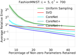
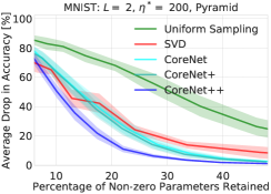
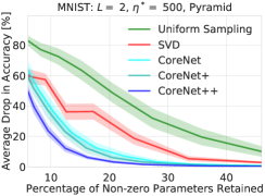
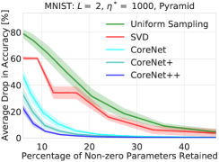
We compare against three variations of our compression algorithm: (i) sole edge sampling (CoreNet), (ii) edge sampling with neuron pruning (CoreNet+), and (iii) edge sampling with neuron pruning and amplification (CoreNet++). For comparison, we evaluated the average relative error in output (1subscript1\ell_{1}-norm) and average drop in classification accuracy relative to the accuracy of the uncompressed network. Both metrics were evaluated on a previously unseen test set.

Results

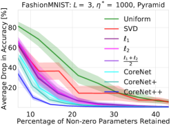
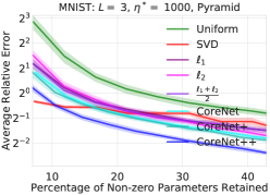
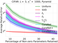
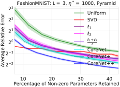
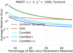
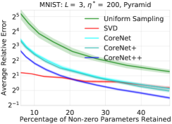
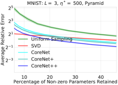
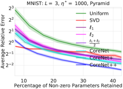
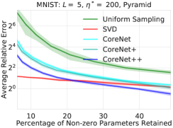
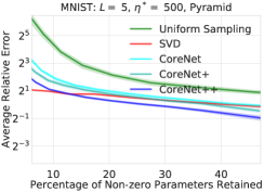
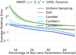
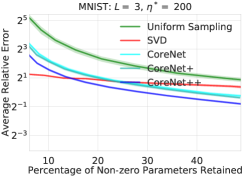
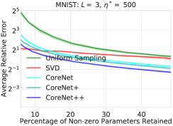
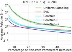
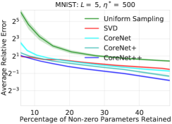
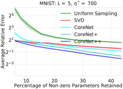
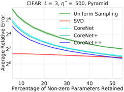
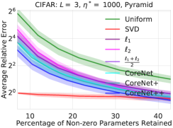
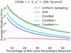
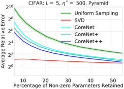
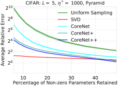
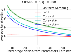
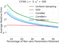
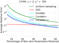
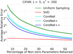
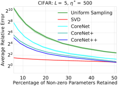
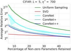
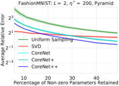
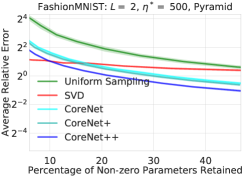
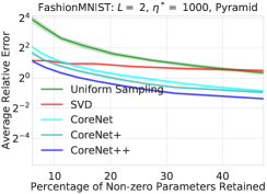
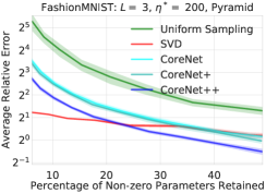
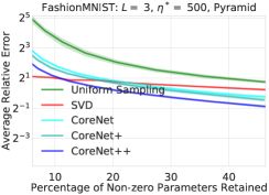
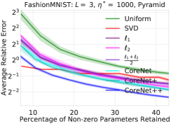
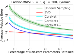
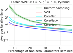
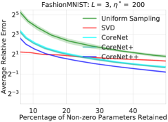
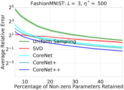
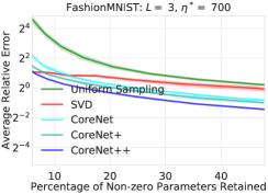
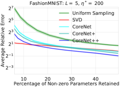
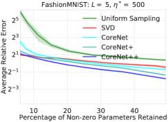
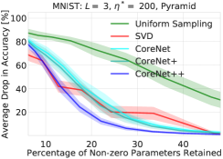
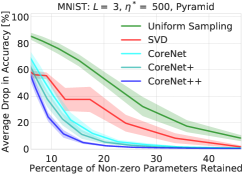
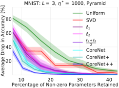
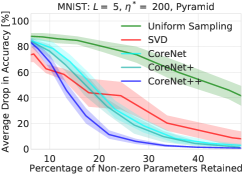
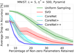
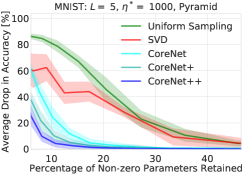
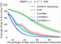
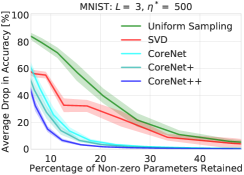
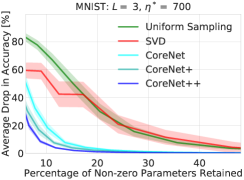
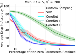
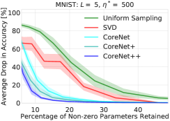
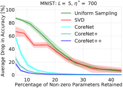
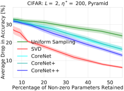
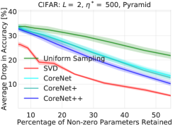
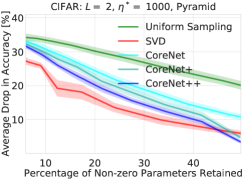
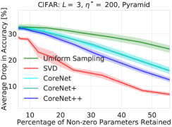
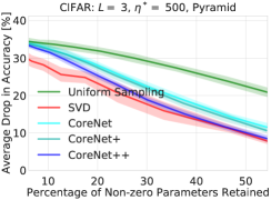
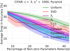
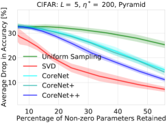
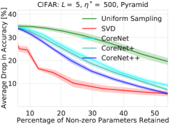
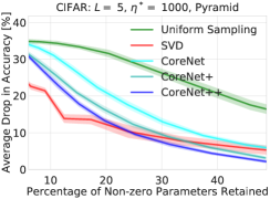
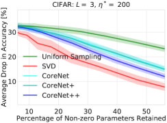
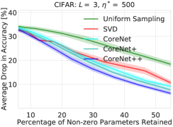
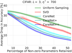
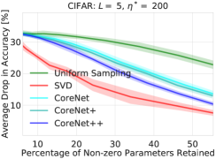
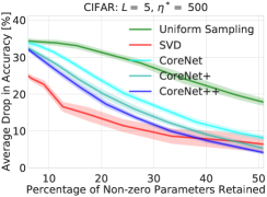
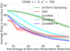
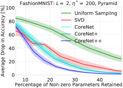
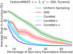
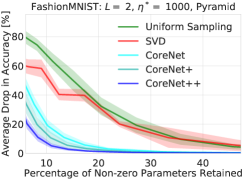
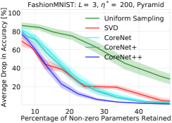
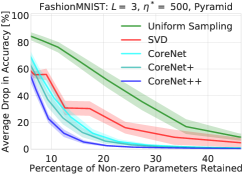
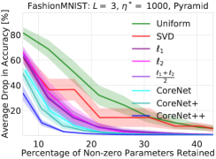
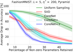
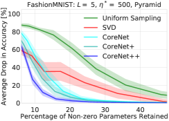
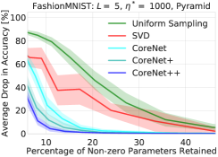
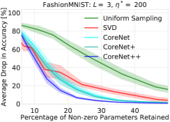
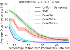
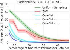
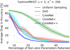
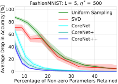
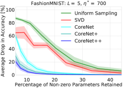
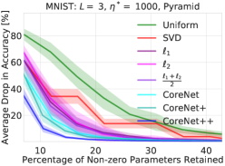
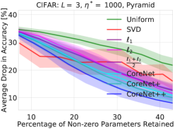
Results for varying architectures and datasets are depicted in Figures 1 and  2 for the average drop in classification accuracy and relative error (1subscript1\ell_{1}-norm), respectively. As apparent from Figure 1, we are able to compress networks to about 15% of their original size without significant loss of accuracy for networks trained on MNIST and FashionMNIST, and to about 50% of their original size for CIFAR.
Refer to caption
Refer to caption
Refer to caption
Figure 1: Evaluation of drop in classification accuracy after compression against the MNIST, CIFAR, and FashionMNIST datasets with varying number of hidden layers (L𝐿L) and number of neurons per hidden layer (ηsuperscript𝜂\eta^{*}). Shaded region corresponds to values within one standard deviation of the mean.
Refer to caption
Refer to caption
Refer to caption
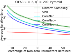
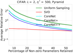
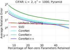
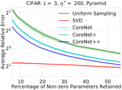
Figure 2: Evaluation of relative error after compression against the MNIST, CIFAR, and FashionMNIST datasets with varying number of hidden layers (L𝐿L) and number of neurons per hidden layer (ηsuperscript𝜂\eta^{*}).
Discussion

The simulation results presented in this section validate our theoretical results established in Sec. 5. In particular, our empirical results indicate that we are able to outperform networks compressed via competing methods in matrix sparsification across all considered experiments and trials. The results presented in this section further suggest that empirical sensitivity can effectively capture the relative importance of neural network parameters, leading to a more informed importance sampling scheme. Moreover, the relative performance of our algorithm tends to increase as we consider deeper architectures. These findings suggest that our algorithm may also be effective in compressing modern convolutional architectures, which tend to be very deep.

7 Conclusion

We presented a coresets-based neural network compression algorithm for compressing the parameters of a trained fully-connected neural network in a manner that approximately preserves the network’s output. Our method and analysis extend traditional coreset constructions to the application of compressing parameters, which may be of independent interest. Our work distinguishes itself from prior approaches in that it establishes theoretical guarantees on the approximation accuracy and size of the generated compressed network. As a corollary to our analysis, we obtain generalization bounds for neural networks, which may provide novel insights on the generalization properties of neural networks. We empirically demonstrated the practical effectiveness of our compression algorithm on a variety of neural network configurations and real-world data sets. In future work, we plan to extend our algorithm and analysis to compress Convolutional Neural Networks (CNNs) and other network architectures. We conjecture that our compression algorithm can be used to reduce storage requirements of neural network models and enable fast inference in practical settings.

Acknowledgments

This research was supported in part by the National Science Foundation award IIS-1723943. We thank Brandon Araki and Kiran Vodrahalli for valuable discussions and helpful suggestions. We would also like to thank Kasper Green Larsen, Alexander Mathiasen, and Allan Gronlund for pointing out an error in an earlier formulation of Lemma 6.

References

  • Achlioptas et al. (2013) Dimitris Achlioptas, Zohar Karnin, and Edo Liberty. Matrix entry-wise sampling: Simple is best. Submitted to KDD, 2013(1.1):1–4, 2013.
  • Agarwal et al. (2005) Pankaj K Agarwal, Sariel Har-Peled, and Kasturi R Varadarajan. Geometric approximation via coresets. Combinatorial and computational geometry, 52:1–30, 2005.
  • Aghasi et al. (2017) Alireza Aghasi, Afshin Abdi, Nam Nguyen, and Justin Romberg. Net-trim: Convex pruning of deep neural networks with performance guarantee. In Advances in Neural Information Processing Systems, pp. 3180–3189, 2017.
  • Alvarez & Salzmann (2017) Jose M Alvarez and Mathieu Salzmann. Compression-aware training of deep networks. In Advances in Neural Information Processing Systems, pp. 856–867, 2017.
  • Arora et al. (2018) Sanjeev Arora, Rong Ge, Behnam Neyshabur, and Yi Zhang. Stronger generalization bounds for deep nets via a compression approach. arXiv preprint arXiv:1802.05296, 2018.
  • Bachem et al. (2017) Olivier Bachem, Mario Lucic, and Andreas Krause. Practical coreset constructions for machine learning. arXiv preprint arXiv:1703.06476, 2017.
  • Badrinarayanan et al. (2015) Vijay Badrinarayanan, Alex Kendall, and Roberto Cipolla. Segnet: A deep convolutional encoder-decoder architecture for image segmentation. CoRR, abs/1511.00561, 2015. URL http://arxiv.org/abs/1511.00561.
  • Bartlett et al. (2017) Peter L Bartlett, Dylan J Foster, and Matus J Telgarsky. Spectrally-normalized margin bounds for neural networks. In Advances in Neural Information Processing Systems, pp. 6241–6250, 2017.
  • Braverman et al. (2016) Vladimir Braverman, Dan Feldman, and Harry Lang. New frameworks for offline and streaming coreset constructions. arXiv preprint arXiv:1612.00889, 2016.
  • Chen et al. (2015a) Wenlin Chen, James T. Wilson, Stephen Tyree, Kilian Q. Weinberger, and Yixin Chen. Compressing convolutional neural networks. CoRR, abs/1506.04449, 2015a. URL http://arxiv.org/abs/1506.04449.
  • Chen et al. (2015b) Wenlin Chen, James T. Wilson, Stephen Tyree, Kilian Q. Weinberger, and Yixin Chen. Compressing neural networks with the hashing trick. CoRR, abs/1504.04788, 2015b. URL http://arxiv.org/abs/1504.04788.
  • Cheng et al. (2015) Yu Cheng, Felix X Yu, Rogerio S Feris, Sanjiv Kumar, Alok Choudhary, and Shi-Fu Chang. An exploration of parameter redundancy in deep networks with circulant projections. In Proceedings of the IEEE International Conference on Computer Vision, pp.  2857–2865, 2015.
  • Choromanska et al. (2016) Anna Choromanska, Krzysztof Choromanski, Mariusz Bojarski, Tony Jebara, Sanjiv Kumar, and Yann LeCun. Binary embeddings with structured hashed projections. In International Conference on Machine Learning, pp. 344–353, 2016.
  • Denil et al. (2013) Misha Denil, Babak Shakibi, Laurent Dinh, Marc Aurelio Ranzato, and Nando de Freitas. Predicting parameters in deep learning. In C. J. C. Burges, L. Bottou, M. Welling, Z. Ghahramani, and K. Q. Weinberger (eds.), Advances in Neural Information Processing Systems 26, pp.  2148–2156. Curran Associates, Inc., 2013. URL http://papers.nips.cc/paper/5025-predicting-parameters-in-deep-learning.pdf.
  • Denton et al. (2014) Emily Denton, Wojciech Zaremba, Joan Bruna, Yann LeCun, and Rob Fergus. Exploiting linear structure within convolutional networks for efficient evaluation. CoRR, abs/1404.0736, 2014. URL http://arxiv.org/abs/1404.0736.
  • Doerr (2018) Benjamin Doerr. Probabilistic tools for the analysis of randomized optimization heuristics. arXiv preprint arXiv:1801.06733, 2018.
  • Dong et al. (2017) Xin Dong, Shangyu Chen, and Sinno Pan. Learning to prune deep neural networks via layer-wise optimal brain surgeon. In Advances in Neural Information Processing Systems, pp. 4860–4874, 2017.
  • Drineas & Zouzias (2011) Petros Drineas and Anastasios Zouzias. A note on element-wise matrix sparsification via a matrix-valued bernstein inequality. Information Processing Letters, 111(8):385–389, 2011.
  • Dziugaite & Roy (2017) Gintare Karolina Dziugaite and Daniel M Roy. Computing nonvacuous generalization bounds for deep (stochastic) neural networks with many more parameters than training data. arXiv preprint arXiv:1703.11008, 2017.
  • Feldman & Langberg (2011) Dan Feldman and Michael Langberg. A unified framework for approximating and clustering data. In Proceedings of the forty-third annual ACM symposium on Theory of computing, pp.  569–578. ACM, 2011.
  • Gong et al. (2014) Yunchao Gong, Liu Liu, Ming Yang, and Lubomir Bourdev. Compressing Deep Convolutional Networks using Vector Quantization. arXiv preprint arXiv:1412.6115, 2014.
  • Han et al. (2015) Song Han, Huizi Mao, and William J. Dally. Deep compression: Compressing deep neural network with pruning, trained quantization and huffman coding. CoRR, abs/1510.00149, 2015. URL http://arxiv.org/abs/1510.00149.
  • Huggins et al. (2016) Jonathan H Huggins, Trevor Campbell, and Tamara Broderick. Coresets for scalable bayesian logistic regression. arXiv preprint arXiv:1605.06423, 2016.
  • Iandola et al. (2016) Forrest N Iandola, Song Han, Matthew W Moskewicz, Khalid Ashraf, William J Dally, and Kurt Keutzer. Squeezenet: Alexnet-level accuracy with 50x fewer parameters and¡ 0.5 mb model size. arXiv preprint arXiv:1602.07360, 2016.
  • Ioannou et al. (2015) Yani Ioannou, Duncan Robertson, Jamie Shotton, Roberto Cipolla, and Antonio Criminisi. Training cnns with low-rank filters for efficient image classification. arXiv preprint arXiv:1511.06744, 2015.
  • Jaderberg et al. (2014) Max Jaderberg, Andrea Vedaldi, and Andrew Zisserman. Speeding up convolutional neural networks with low rank expansions. arXiv preprint arXiv:1405.3866, 2014.
  • Johnson & Lindenstrauss (1984) William B Johnson and Joram Lindenstrauss. Extensions of lipschitz mappings into a hilbert space. Contemporary mathematics, 26(189-206):1, 1984.
  • Kim et al. (2015) Yong-Deok Kim, Eunhyeok Park, Sungjoo Yoo, Taelim Choi, Lu Yang, and Dongjun Shin. Compression of deep convolutional neural networks for fast and low power mobile applications. arXiv preprint arXiv:1511.06530, 2015.
  • Krizhevsky & Hinton (2009) Alex Krizhevsky and Geoffrey Hinton. Learning multiple layers of features from tiny images. 2009.
  • Krizhevsky et al. (2012) Alex Krizhevsky, Ilya Sutskever, and Geoffrey E Hinton. Imagenet classification with deep convolutional neural networks. In F. Pereira, C. J. C. Burges, L. Bottou, and K. Q. Weinberger (eds.), Advances in Neural Information Processing Systems 25, pp. 1097–1105. Curran Associates, Inc., 2012. URL http://papers.nips.cc/paper/4824-imagenet-classification-with-deep-convolutional-neural-networks.pdf.
  • Kundu & Drineas (2014) Abhisek Kundu and Petros Drineas. A note on randomized element-wise matrix sparsification. arXiv preprint arXiv:1404.0320, 2014.
  • Langberg & Schulman (2010) Michael Langberg and Leonard J Schulman. Universal ε𝜀\varepsilon-approximators for integrals. In Proceedings of the twenty-first annual ACM-SIAM symposium on Discrete Algorithms, pp.  598–607. SIAM, 2010.
  • Lebedev & Lempitsky (2016) Vadim Lebedev and Victor Lempitsky. Fast convnets using group-wise brain damage. In Computer Vision and Pattern Recognition (CVPR), 2016 IEEE Conference on, pp.  2554–2564. IEEE, 2016.
  • LeCun et al. (1990) Yann LeCun, John S Denker, and Sara A Solla. Optimal brain damage. In Advances in neural information processing systems, pp. 598–605, 1990.
  • LeCun et al. (1998) Yann LeCun, Léon Bottou, Yoshua Bengio, and Patrick Haffner. Gradient-based learning applied to document recognition. Proceedings of the IEEE, 86(11):2278–2324, 1998.
  • Lin et al. (2017) Ji Lin, Yongming Rao, Jiwen Lu, and Jie Zhou. Runtime neural pruning. In Advances in Neural Information Processing Systems, pp. 2178–2188, 2017.
  • Long et al. (2015) Jonathan Long, Evan Shelhamer, and Trevor Darrell. Fully convolutional networks for semantic segmentation. In The IEEE Conference on Computer Vision and Pattern Recognition (CVPR), June 2015.
  • Molina et al. (2018) Alejandro Molina, Alexander Munteanu, and Kristian Kersting. Core dependency networks. In Proceedings of the 32nd AAAI Conference on Artificial Intelligence (AAAI). AAAI Press Google Scholar, 2018.
  • Munteanu & Schwiegelshohn (2018) Alexander Munteanu and Chris Schwiegelshohn. Coresets-methods and history: A theoreticians design pattern for approximation and streaming algorithms. KI-Künstliche Intelligenz, 32(1):37–53, 2018.
  • Neyshabur et al. (2017a) Behnam Neyshabur, Srinadh Bhojanapalli, David McAllester, and Nathan Srebro. A pac-bayesian approach to spectrally-normalized margin bounds for neural networks. arXiv preprint arXiv:1707.09564, 2017a.
  • Neyshabur et al. (2017b) Behnam Neyshabur, Srinadh Bhojanapalli, David McAllester, and Nati Srebro. Exploring generalization in deep learning. In Advances in Neural Information Processing Systems, pp. 5949–5958, 2017b.
  • Paszke et al. (2017) Adam Paszke, Sam Gross, Soumith Chintala, Gregory Chanan, Edward Yang, Zachary DeVito, Zeming Lin, Alban Desmaison, Luca Antiga, and Adam Lerer. Automatic differentiation in pytorch. In NIPS-W, 2017.
  • Shi et al. (2009) Qinfeng Shi, James Petterson, Gideon Dror, John Langford, Alex Smola, and SVN Vishwanathan. Hash kernels for structured data. Journal of Machine Learning Research, 10(Nov):2615–2637, 2009.
  • Sindhwani et al. (2015) Vikas Sindhwani, Tara Sainath, and Sanjiv Kumar. Structured transforms for small-footprint deep learning. In Advances in Neural Information Processing Systems, pp. 3088–3096, 2015.
  • Tai et al. (2015) Cheng Tai, Tong Xiao, Yi Zhang, Xiaogang Wang, et al. Convolutional neural networks with low-rank regularization. arXiv preprint arXiv:1511.06067, 2015.
  • Ullrich et al. (2017) Karen Ullrich, Edward Meeds, and Max Welling. Soft weight-sharing for neural network compression. arXiv preprint arXiv:1702.04008, 2017.
  • Vershynin (2016) Roman Vershynin. High-dimensional probability. An Introduction with Applications, 2016.
  • Weinberger et al. (2009) Kilian Q. Weinberger, Anirban Dasgupta, Josh Attenberg, John Langford, and Alexander J. Smola. Feature hashing for large scale multitask learning. CoRR, abs/0902.2206, 2009. URL http://arxiv.org/abs/0902.2206.
  • Wen et al. (2016) Wei Wen, Chunpeng Wu, Yandan Wang, Yiran Chen, and Hai Li. Learning structured sparsity in deep neural networks. In Advances in Neural Information Processing Systems, pp. 2074–2082, 2016.
  • Wu et al. (2016) Jiaxiang Wu, Cong Leng, Yuhang Wang, Qinghao Hu, and Jian Cheng. Quantized Convolutional Neural Networks for Mobile Devices. In Proceedings of the Inernational Conference on Computer Vision and Pattern Recognition (CVPR), 2016.
  • Xiao et al. (2017) Han Xiao, Kashif Rasul, and Roland Vollgraf. Fashion-mnist: a novel image dataset for benchmarking machine learning algorithms, 2017.
  • Yu et al. (2017) Xiyu Yu, Tongliang Liu, Xinchao Wang, and Dacheng Tao. On compressing deep models by low rank and sparse decomposition. In Proceedings of the IEEE Conference on Computer Vision and Pattern Recognition, pp.  7370–7379, 2017.
  • Zhao et al. (2017) Liang Zhao, Siyu Liao, Yanzhi Wang, Jian Tang, and Bo Yuan. Theoretical properties for neural networks with weight matrices of low displacement rank. CoRR, abs/1703.00144, 2017. URL http://arxiv.org/abs/1703.00144.
  • Zhou et al. (2017) Aojun Zhou, Anbang Yao, Yiwen Guo, Lin Xu, and Yurong Chen. Incremental Network Quantization: Towards Lossless CNNs with Low-Precision Weights. In Proceedings of the International Conference on Learning Representations (ICLR) 2017, feb 2017.
  • Zhou et al. (2018) Wenda Zhou, Victor Veitch, Morgane Austern, Ryan P Adams, and Peter Orbanz. Compressibility and generalization in large-scale deep learning. arXiv preprint arXiv:1804.05862, 2018.

Appendix A Proofs of the Analytical Results in Section 5

This section includes the full proofs of the technical results given in Sec. 5.

A.1 Analytical Results for Section 5.2 (Importance Sampling Bounds for Positive Weights)

A.1.1 Order Statistic Sampling

We now establish a couple of technical results that will quantify the accuracy of our approximations of edge importance (i.e., sensitivity).

Lemma 6.

Let K,K>0𝐾superscript𝐾0K,K^{\prime}>0 be universal constants and let 𝒟𝒟{\mathcal{D}} be a distribution with CDF F()𝐹F(\cdot) satisfying F(M/K)exp(1/K)𝐹𝑀𝐾1superscript𝐾F(\nicefrac{{M}}{{K}})\leq\exp(-1/K^{\prime}), where M=min{x[0,1]:F(x)=1}𝑀:𝑥01𝐹𝑥1M=\min\{x\in[0,1]:F(x)=1\}. Let 𝒫={X1,,Xn}𝒫subscript𝑋1subscript𝑋𝑛\mathcal{P}=\{X_{1},\ldots,X_{n}\} be a set of n=|𝒫|𝑛𝒫n=|\mathcal{P}| i.i.d. samples each drawn from the distribution 𝒟𝒟{\mathcal{D}}. Let Xn+1𝒟similar-tosubscript𝑋𝑛1𝒟X_{n+1}\sim{\mathcal{D}} be an i.i.d. sample. Then,

(KmaxX𝒫X<Xn+1)exp(n/K)𝐾subscript𝑋𝒫𝑋subscript𝑋𝑛1𝑛𝐾\displaystyle\operatorname*{\mathbb{P}}\left(K\,\max_{X\in\mathcal{P}}X<X_{n+1}\right)\leq\exp(-n/K)
Proof.

Let Xmax=maxX𝒫subscript𝑋maxsubscript𝑋𝒫X_{\mathrm{max}}=\max_{X\in\mathcal{P}}; then,

(KXmax<Xn+1)𝐾subscript𝑋maxsubscript𝑋𝑛1\displaystyle\operatorname*{\mathbb{P}}(K\,X_{\mathrm{max}}<X_{n+1}) =0M(Xmax<x/K|Xn+1=x)d(x)absentsuperscriptsubscript0𝑀subscript𝑋maxbra𝑥𝐾subscript𝑋𝑛1𝑥𝑑𝑥\displaystyle=\int_{0}^{M}\operatorname*{\mathbb{P}}(X_{\mathrm{max}}<\nicefrac{{x}}{{K}}|X_{n+1}=x)\,d\operatorname*{\mathbb{P}}(x)
=0M(X<x/K)nd(x)\displaystyle=\int_{0}^{M}\operatorname*{\mathbb{P}}\left(X<\nicefrac{{x}}{{K}}\right)^{n}\,d\operatorname*{\mathbb{P}}(x) since X1,,Xnsubscript𝑋1subscript𝑋𝑛X_{1},\ldots,X_{n} are i.i.d.
0MF(x/K)nd(x)absentsuperscriptsubscript0𝑀𝐹superscript𝑥𝐾𝑛𝑑𝑥\displaystyle\leq\int_{0}^{M}F(\nicefrac{{x}}{{K}})^{n}\,d\operatorname*{\mathbb{P}}(x) where F()𝐹F(\cdot) is the CDF of X𝒟similar-to𝑋𝒟X\sim{\mathcal{D}}
F(M/K)n0Md(x)absent𝐹superscript𝑀𝐾𝑛superscriptsubscript0𝑀𝑑𝑥\displaystyle\leq F(\nicefrac{{M}}{{K}})^{n}\int_{0}^{M}\,d\operatorname*{\mathbb{P}}(x) by monotonicity of F𝐹F
=F(M/K)nabsent𝐹superscript𝑀𝐾𝑛\displaystyle=F(\nicefrac{{M}}{{K}})^{n}
exp(n/K)absent𝑛superscript𝐾\displaystyle\leq\exp(-n/K^{\prime}) CDF Assumption,CDF Assumption\displaystyle\text{CDF Assumption},

and this completes the proof. ∎

We now proceed to establish that the notion of empirical sensitivity is a good approximation for the relative importance. For this purpose, let the relative importance g^j(x)subscript^𝑔𝑗𝑥\hat{g}_{j}(x) of an edge j𝑗j after the previous layers have already been compressed be

g^j(x)=wja^j(x)k𝒲wka^k(x).subscript^𝑔𝑗𝑥subscript𝑤𝑗subscript^𝑎𝑗𝑥subscript𝑘𝒲subscript𝑤𝑘subscript^𝑎𝑘𝑥\hat{g}_{j}(x)=\frac{w_{j}\,\hat{a}_{j}(x)}{\sum_{k\in\mathcal{W}}w_{k}\,\hat{a}_{k}(x)}.
Lemma 7 (Empirical Sensitivity Approximation).

Let ε(0,1/2),δ(0,1)formulae-sequence𝜀012𝛿01\varepsilon\in(0,1/2),\delta\in(0,1), {2,,L}2𝐿\ell\in\left\{2,\ldots,L\right\}, Consider a set SS={x1,,xn}𝒫SSsubscript𝑥1subscript𝑥𝑛𝒫\SS=\{x_{1},\ldots,x_{n}\}\subseteq\mathcal{P} of size |SS|Klog(8ηη/δ)SSsuperscript𝐾8𝜂superscript𝜂𝛿|\SS|\geq\left\lceil K^{\prime}\log\left(8\,\eta\,\eta^{*}/\delta\right)\right\rceil. Then, conditioned on the event 1/2subscript12\mathcal{E}_{\nicefrac{{1}}{{2}}} occurring, i.e., a^(x)(1±1/2)a(x)^𝑎𝑥plus-or-minus112𝑎𝑥\hat{a}(x)\in(1\pm\nicefrac{{1}}{{2}})a(x),

x𝒟(j𝒲:Csj<g^j(x)1/2)δ8η,subscriptsimilar-to𝑥𝒟:𝑗𝒲𝐶subscript𝑠𝑗brasubscript^𝑔𝑗𝑥subscript12𝛿8𝜂\operatorname*{\mathbb{P}}_{x\sim{\mathcal{D}}}\left(\exists{j\in\mathcal{W}}:C\,s_{j}<\hat{g}_{j}(x)\,\mid\,\mathcal{E}_{\nicefrac{{1}}{{2}}}\right)\leq\frac{\delta}{8\,\eta},

where C=3K𝐶3𝐾C=3\,K and 𝒲[η1]𝒲delimited-[]superscript𝜂1\mathcal{W}\subseteq[\eta^{\ell-1}].

Proof.

Consider an arbitrary j𝒲𝑗𝒲j\in\mathcal{W} and xSSsuperscript𝑥SSx^{\prime}\in\SS corresponding to gj(x)subscript𝑔𝑗superscript𝑥g_{j}(x^{\prime}) with CDF Fj()subscript𝐹𝑗F_{j}\left(\cdot\right) and recall that M=min{x[0,1]:Fj(x)=1}𝑀:𝑥01subscript𝐹𝑗𝑥1M=\min\{x\in[0,1]:F_{j}\left(x\right)=1\} as in Assumption 1. Note that by Assumption 1, we have

F(M/K)exp(1/K),𝐹𝑀𝐾1superscript𝐾F(\nicefrac{{M}}{{K}})\leq\exp(-1/K^{\prime}),

and so the random variables gj(x)subscript𝑔𝑗superscript𝑥g_{j}(x^{\prime}) for xSSsuperscript𝑥SSx^{\prime}\in\SS satisfy the CDF condition required by Lemma 6. Now let \mathcal{E} be the event that Ksj<gj(x)𝐾subscript𝑠𝑗subscript𝑔𝑗𝑥K\,s_{j}<g_{j}(x) holds. Applying Lemma 6, we obtain

()\displaystyle\operatorname*{\mathbb{P}}(\mathcal{E}) =(Ksj<gj(x))=(KmaxxSSgj(x)<gj(x))exp(|SS|/K).absent𝐾subscript𝑠𝑗subscript𝑔𝑗𝑥𝐾subscriptsuperscript𝑥SSsubscript𝑔𝑗superscript𝑥subscript𝑔𝑗𝑥SSsuperscript𝐾\displaystyle=\operatorname*{\mathbb{P}}(K\,s_{j}<g_{j}(x))=\operatorname*{\mathbb{P}}\left(K\,\max_{x^{\prime}\in\SS}g_{j}(x^{\prime})<g_{j}(x)\right)\leq\exp(-|\SS|/K^{\prime}).

Now let ^^\hat{\mathcal{E}} denote the event that the inequality Csj<g^j(x)=wja^j(x)k𝒲wka^k(x)𝐶subscript𝑠𝑗subscript^𝑔𝑗𝑥subscript𝑤𝑗subscript^𝑎𝑗𝑥subscript𝑘𝒲subscript𝑤𝑘subscript^𝑎𝑘𝑥Cs_{j}<\hat{g}_{j}(x)=\frac{w_{j}\,\hat{a}_{j}(x)}{\sum_{k\in\mathcal{W}}w_{k}\,\hat{a}_{k}(x)} holds and note that the right side of the inequality is defined with respect to g^j(x)subscript^𝑔𝑗𝑥\hat{g}_{j}(x) and not gj(x)subscript𝑔𝑗𝑥g_{j}(x). Observe that since we conditioned on the event 1/2subscript12\mathcal{E}_{\nicefrac{{1}}{{2}}}, we have that a^(x)(1±1/2)a(x).^𝑎𝑥plus-or-minus112𝑎𝑥\hat{a}(x)\in(1\pm\nicefrac{{1}}{{2}})a(x).

Now assume that event ^^\hat{\mathcal{E}} holds and note that by the implication above, we have

Csj<g^j(x)𝐶subscript𝑠𝑗subscript^𝑔𝑗𝑥\displaystyle C\,s_{j}<\hat{g}_{j}(x) =wja^j(x)k𝒲wka^k(x)(1+1/2)wjaj(x)(11/2)k𝒲wkak(x)absentsubscript𝑤𝑗subscript^𝑎𝑗𝑥subscript𝑘𝒲subscript𝑤𝑘subscript^𝑎𝑘𝑥112subscript𝑤𝑗subscript𝑎𝑗𝑥112subscript𝑘𝒲subscript𝑤𝑘subscript𝑎𝑘𝑥\displaystyle=\frac{w_{j}\,\hat{a}_{j}(x)}{\sum_{k\in\mathcal{W}}w_{k}\,\hat{a}_{k}(x)}\leq\frac{(1+\nicefrac{{1}}{{2}})w_{j}\,a_{j}(x)}{(1-\nicefrac{{1}}{{2}})\sum_{k\in\mathcal{W}}w_{k}\,a_{k}(x)}
3wjaj(x)k𝒲wkak(x)=3gj(x).absent3subscript𝑤𝑗subscript𝑎𝑗𝑥subscript𝑘𝒲subscript𝑤𝑘subscript𝑎𝑘𝑥3subscript𝑔𝑗𝑥\displaystyle\leq 3\cdot\frac{w_{j}\,a_{j}(x)}{\sum_{k\in\mathcal{W}}w_{k}\,a_{k}(x)}=3\,g_{j}(x).

where the second inequality follows from the fact that 1+1/2/11/231121123\nicefrac{{1+1/2}}{{1-1/2}}\leq 3. Moreover, since we know that C3K𝐶3𝐾C\geq 3K, we conclude that if event ^^\hat{\mathcal{E}} occurs, we obtain the inequality

3Ksj3gj(x)Ksjgj(x),3𝐾subscript𝑠𝑗3subscript𝑔𝑗𝑥𝐾subscript𝑠𝑗subscript𝑔𝑗𝑥3\,K\,s_{j}\leq 3\,g_{j}(x)\Leftrightarrow K\,s_{j}\leq g_{j}(x),

which is precisely the definition of event \mathcal{E}. Thus, we have shown the conditional implication (^1/2)conditional^subscript12\big{(}\hat{\mathcal{E}}\,\mid\,\mathcal{E}_{\nicefrac{{1}}{{2}}}\big{)}\Rightarrow\mathcal{E}, which implies that

(^1/2)conditional^subscript12\displaystyle\operatorname*{\mathbb{P}}(\hat{\mathcal{E}}\,\mid\,\mathcal{E}_{\nicefrac{{1}}{{2}}}) =(Csj<g^j(x)1/2)()absent𝐶subscript𝑠𝑗brasubscript^𝑔𝑗𝑥subscript12\displaystyle=\operatorname*{\mathbb{P}}(C\,s_{j}<\hat{g}_{j}(x)\,\mid\,\mathcal{E}_{\nicefrac{{1}}{{2}}})\leq\operatorname*{\mathbb{P}}(\mathcal{E})
exp(|SS|/K).absentSSsuperscript𝐾\displaystyle\leq\exp(-|\SS|/K^{\prime}).

Since our choice of j𝒲𝑗𝒲j\in\mathcal{W} was arbitrary, the bound applies for any j𝒲𝑗𝒲j\in\mathcal{W}. Thus, we have by the union bound

(j𝒲:Csj<g^j(x)1/2):𝑗𝒲𝐶subscript𝑠𝑗brasubscript^𝑔𝑗𝑥subscript12\displaystyle\operatorname*{\mathbb{P}}(\exists{j\in\mathcal{W}}\,:C\,s_{j}<\hat{g}_{j}(x)\,\mid\,\mathcal{E}_{\nicefrac{{1}}{{2}}}) j𝒲(Csj<g^j(x)1/2)|𝒲|exp(|SS|/K)absentsubscript𝑗𝒲𝐶subscript𝑠𝑗brasubscript^𝑔𝑗𝑥subscript12𝒲SSsuperscript𝐾\displaystyle\leq\sum_{j\in\mathcal{W}}\operatorname*{\mathbb{P}}(C\,s_{j}<\hat{g}_{j}(x)\,\mid\,\mathcal{E}_{\nicefrac{{1}}{{2}}})\leq\left|\mathcal{W}\right|\exp(-|\SS|/K^{\prime})
=(|𝒲|η)δ8ηδ8η.absent𝒲superscript𝜂𝛿8𝜂𝛿8𝜂\displaystyle=\left(\frac{|\mathcal{W}|}{\eta^{*}}\right)\frac{\delta}{8\eta}\leq\frac{\delta}{8\eta}.

In practice, the set SSSS\SS referenced above is chosen to be a subset of the original data points, i.e., SS𝒫SS𝒫\SS\subseteq\mathcal{P} (see Alg. 1, Line 2). Thus, we henceforth assume that the size of the input points |𝒫|𝒫|\mathcal{P}| is large enough (or the specified parameter δ(0,1)𝛿01\delta\in(0,1) is sufficiently large) so that |𝒫||SS|𝒫SS|\mathcal{P}|\geq|\SS|.

A.1.2 Proof of Lemma 1

We now state the proof of Lemma 1. In this subsection, we establish approximation guarantees under the assumption that the weights are strictly positive. The next subsection will then relax this assumption to conclude that a neuron’s value can be approximated well even when the weights are not all positive.

See 1

Proof.

Let ε,δ(0,1)𝜀𝛿01\varepsilon,\delta\in(0,1) be arbitrary. Moreover, let 𝒞𝒞\mathcal{C} be the coreset with respect to the weight indices 𝒲[η1]𝒲delimited-[]superscript𝜂1\mathcal{W}\subseteq[\eta^{\ell-1}] used to construct w^^𝑤{\hat{w}}. Note that as in Sparsify, 𝒞𝒞\mathcal{C} is a multiset sampled from 𝒲𝒲\mathcal{W} of size m=8SKlog(8η/δ)ε2,𝑚8𝑆𝐾8𝜂𝛿superscript𝜀2m=\left\lceil\frac{8\,S\,K\log({8\,\eta/\delta})}{{\varepsilon}^{2}}\right\rceil, where S=j𝒲sj𝑆subscript𝑗𝒲subscript𝑠𝑗S=\sum_{j\in\mathcal{W}}s_{j} and 𝒞𝒞\mathcal{C} is sampled according to the probability distribution q𝑞q defined by

qj=sjSj𝒲.formulae-sequencesubscript𝑞𝑗subscript𝑠𝑗𝑆for-all𝑗𝒲q_{j}=\frac{s_{j}}{S}\qquad\forall{j\in\mathcal{W}}.

Let 𝐚^()^𝐚\mathbf{\hat{a}}(\cdot) be an arbitrary realization of the random variable a^1()superscript^𝑎1\hat{a}^{\ell-1}(\cdot), let 𝐱𝐱\mathbf{x} be a realization of x𝒟similar-to𝑥𝒟x\sim{\mathcal{D}}, and let

z^=k𝒲w^k𝐚^k(𝐱)^𝑧subscript𝑘𝒲subscript^𝑤𝑘subscript^𝐚𝑘𝐱\hat{z}=\sum_{k\in\mathcal{W}}{\hat{w}_{k}}\,\mathbf{\hat{a}}_{k}(\mathbf{x})

be the approximate intermediate value corresponding to the sparsified matrix w^^𝑤{\hat{w}} and let

z~=k𝒲wk𝐚^k(𝐱).~𝑧subscript𝑘𝒲subscript𝑤𝑘subscript^𝐚𝑘𝐱\tilde{z}=\sum_{k\in\mathcal{W}}w_{k}\,\mathbf{\hat{a}}_{k}(\mathbf{x}).

Now define \mathcal{E} to be the (favorable) event that z^^𝑧\hat{z} ε𝜀\varepsilon-approximates z~~𝑧\tilde{z}, i.e., z^(1±ε)z~^𝑧plus-or-minus1𝜀~𝑧\hat{z}\in(1\pm\varepsilon)\tilde{z}, We will now show that the complement of this event, 𝖼superscript𝖼\mathcal{E}^{\mathsf{c}}, occurs with sufficiently small probability. Let 𝒵supp(𝒟)𝒵supp𝒟{\mathcal{Z}}\subseteq\mathrm{supp}({\mathcal{D}}) be the set of well-behaved points (defined implicitly with respect to neuron i[η]𝑖delimited-[]superscript𝜂i\in[\eta^{\ell}] and realization 𝐚^^𝐚\mathbf{\hat{a}}) and defined as follows:

𝒵={xsupp(𝒟):g^j(x)Csjj𝒲},𝒵conditional-setsuperscript𝑥supp𝒟subscript^𝑔𝑗superscript𝑥𝐶subscript𝑠𝑗for-all𝑗𝒲{\mathcal{Z}}=\left\{x^{\prime}\in\mathrm{supp}({\mathcal{D}})\,:\,\hat{g}_{j}(x^{\prime})\leq Cs_{j}\quad\forall{j\in\mathcal{W}}\right\},

where C=3K𝐶3𝐾C=3\,K. Let 𝒵subscript𝒵\mathcal{E}_{{\mathcal{Z}}} denote the event that 𝐱𝒵𝐱𝒵\mathbf{x}\in{\mathcal{Z}} where 𝐱𝐱\mathbf{x} is a realization of x𝒟similar-to𝑥𝒟x\sim{\mathcal{D}}.

Conditioned on 𝒵subscript𝒵\mathcal{E}_{\mathcal{Z}}, event 𝖼superscript𝖼\mathcal{E}^{\mathsf{c}} occurs with probability δ4ηabsent𝛿4𝜂\leq\frac{\delta}{4\eta}:

Let 𝐱𝐱\mathbf{x} be a realization of x𝒟similar-to𝑥𝒟x\sim{\mathcal{D}} such that 𝐱𝒵𝐱𝒵\mathbf{x}\in{\mathcal{Z}} and let 𝒞={c1,,cm}𝒞subscript𝑐1subscript𝑐𝑚\mathcal{C}=\{c_{1},\ldots,c_{m}\} be m𝑚m samples from 𝒲𝒲\mathcal{W} with respect to distribution q𝑞q as before. Define m𝑚m random variables Tc1,,Tcmsubscript𝑇subscript𝑐1subscript𝑇subscript𝑐𝑚T_{c_{1}},\ldots,T_{c_{m}} such that for all j𝒞𝑗𝒞j\in\mathcal{C}

Tjsubscript𝑇𝑗\displaystyle T_{j} =wj𝐚^j(𝐱)mqj=Swj𝐚^j(𝐱)msj.absentsubscript𝑤𝑗subscript^𝐚𝑗𝐱𝑚subscript𝑞𝑗𝑆subscript𝑤𝑗subscript^𝐚𝑗𝐱𝑚subscript𝑠𝑗\displaystyle=\frac{w_{j}\,\mathbf{\hat{a}}_{j}(\mathbf{x})}{m\,q_{j}}=\frac{S\,w_{j}\,\mathbf{\hat{a}}_{j}(\mathbf{x})}{m\,s_{j}}. (2)

For any j𝒞𝑗𝒞j\in\mathcal{C}, we have for the conditional expectation of Tjsubscript𝑇𝑗T_{j}:

𝔼[Tj𝐚^(),𝐱,𝒵,1/2]𝔼conditionalsubscript𝑇𝑗^𝐚𝐱subscript𝒵subscript12\displaystyle\operatorname*{\mathbb{E}\,}[T_{j}\,\mid\,\mathbf{\hat{a}}(\cdot),\mathbf{x},\mathcal{E}_{\mathcal{Z}},\mathcal{E}_{\nicefrac{{1}}{{2}}}] =k𝒲wk𝐚^k(𝐱)mqkqkabsentsubscript𝑘𝒲subscript𝑤𝑘subscript^𝐚𝑘𝐱𝑚subscript𝑞𝑘subscript𝑞𝑘\displaystyle=\sum_{k\in\mathcal{W}}\frac{w_{k}\,\mathbf{\hat{a}}_{k}(\mathbf{x})}{m\,q_{k}}\cdot q_{k}
=k𝒲wk𝐚^k(𝐱)mabsentsubscript𝑘𝒲subscript𝑤𝑘subscript^𝐚𝑘𝐱𝑚\displaystyle=\sum_{k\in\mathcal{W}}\frac{w_{k}\,\mathbf{\hat{a}}_{k}(\mathbf{x})}{m}
=z~m,absent~𝑧𝑚\displaystyle=\frac{\tilde{z}}{m},

where we use the expectation notation 𝔼[]𝔼\operatorname*{\mathbb{E}\,}[\cdot] with the understanding that it denotes the conditional expectation 𝔼𝒞a^l1(),x[]subscript𝔼conditional𝒞superscript^𝑎𝑙1𝑥\operatorname*{\mathbb{E}\,}\nolimits_{\mathcal{C}\,\mid\,\hat{a}^{l-1}(\cdot),\,x}\,[\cdot]. Moreover, we also note that conditioning on the event 𝒵subscript𝒵\mathcal{E}_{\mathcal{Z}} (i.e., the event that 𝐱𝒵𝐱𝒵\mathbf{x}\in{\mathcal{Z}}) does not affect the expectation of Tjsubscript𝑇𝑗T_{j}. Let T=j𝒞Tj=z^𝑇subscript𝑗𝒞subscript𝑇𝑗^𝑧T=\sum_{j\in\mathcal{C}}T_{j}=\hat{z} denote our approximation and note that by linearity of expectation,

𝔼[T𝐚^(),𝐱,𝒵,1/2]=j𝒞𝔼[Tj𝐚^(),𝐱,𝒵,1/2]=z~𝔼conditional𝑇^𝐚𝐱subscript𝒵subscript12subscript𝑗𝒞𝔼conditionalsubscript𝑇𝑗^𝐚𝐱subscript𝒵subscript12~𝑧\operatorname*{\mathbb{E}\,}[T\,\mid\,\mathbf{\hat{a}}(\cdot),\mathbf{x},\mathcal{E}_{\mathcal{Z}},\mathcal{E}_{\nicefrac{{1}}{{2}}}]=\sum_{j\in\mathcal{C}}\operatorname*{\mathbb{E}\,}[T_{j}\,\mid\,\mathbf{\hat{a}}(\cdot),\mathbf{x},\mathcal{E}_{\mathcal{Z}},\mathcal{E}_{\nicefrac{{1}}{{2}}}]=\tilde{z}

Thus, z^=T^𝑧𝑇\hat{z}=T is an unbiased estimator of z~~𝑧\tilde{z} for any realization 𝐚^()^𝐚\mathbf{\hat{a}}(\cdot) and 𝐱𝐱\mathbf{x}; thus, we will henceforth refer to 𝔼[T𝐚^(),𝐱]𝔼conditional𝑇^𝐚𝐱\operatorname*{\mathbb{E}\,}[T\,\mid\,\mathbf{\hat{a}}(\cdot),\,\mathbf{x}] as simply z~~𝑧\tilde{z} for brevity.

For the remainder of the proof we will assume that z~>0~𝑧0\tilde{z}>0, since otherwise, z~=0~𝑧0\tilde{z}=0 if and only if Tj=0subscript𝑇𝑗0T_{j}=0 for all j𝒞𝑗𝒞j\in\mathcal{C} almost surely, which follows by the fact that Tj0subscript𝑇𝑗0T_{j}\geq 0 for all j𝒞𝑗𝒞j\in\mathcal{C} by definition of 𝒲𝒲\mathcal{W} and the non-negativity of the ReLU activation. Therefore, in the case that z~=0~𝑧0\tilde{z}=0, it follows that

(|z^z~|>εz~𝐚^(),𝐱)=(z^>0𝐚^(),𝐱)=(0>0)=0,^𝑧~𝑧conditional𝜀~𝑧^𝐚𝐱^𝑧conditional0^𝐚𝐱000\operatorname*{\mathbb{P}}(|\hat{z}-\tilde{z}|>\varepsilon\tilde{z}\,\mid\,\mathbf{\hat{a}}(\cdot),\mathbf{x})=\operatorname*{\mathbb{P}}(\hat{z}>0\,\mid\,\mathbf{\hat{a}}(\cdot),\mathbf{x})=\operatorname*{\mathbb{P}}(0>0)=0,

which trivially yields the statement of the lemma, where in the above expression, ()\operatorname*{\mathbb{P}}(\cdot) is short-hand for the conditional probability w^a^l1(),x()subscriptconditional^𝑤superscript^𝑎𝑙1𝑥\operatorname*{\mathbb{P}}_{{\hat{w}}\,\mid\,\hat{a}^{l-1}(\cdot),\,x}(\cdot).

We now proceed with the case where z~>0~𝑧0\tilde{z}>0 and leverage the fact that 𝐱𝒵𝐱𝒵\mathbf{x}\in{\mathcal{Z}}333Since we conditioned on the event 𝒵subscript𝒵\mathcal{E}_{\mathcal{Z}}. to establish that for all j𝒲𝑗𝒲j\in\mathcal{W}:

Csj𝐶subscript𝑠𝑗\displaystyle Cs_{j} g^j(𝐱)=wj𝐚^j(𝐱)k𝒲wk𝐚^k(𝐱)=wj𝐚^j(𝐱)z~absentsubscript^𝑔𝑗𝐱subscript𝑤𝑗subscript^𝐚𝑗𝐱subscript𝑘𝒲subscript𝑤𝑘subscript^𝐚𝑘𝐱subscript𝑤𝑗subscript^𝐚𝑗𝐱~𝑧\displaystyle\geq\hat{g}_{j}(\mathbf{x})=\frac{w_{j}\,\mathbf{\hat{a}}_{j}(\mathbf{x})}{\sum_{k\in\mathcal{W}}w_{k}\,\mathbf{\hat{a}}_{k}(\mathbf{x})}=\frac{w_{j}\,\mathbf{\hat{a}}_{j}(\mathbf{x})}{\tilde{z}}
wj𝐚^j(𝐱)sjabsentsubscript𝑤𝑗subscript^𝐚𝑗𝐱subscript𝑠𝑗\displaystyle\Leftrightarrow\quad\frac{w_{j}\,\mathbf{\hat{a}}_{j}(\mathbf{x})}{s_{j}} Cz~.absent𝐶~𝑧\displaystyle\leq C\,\tilde{z}. (3)

Utilizing the inequality established above, we bound the conditional variance of each Tj,j𝒞subscript𝑇𝑗𝑗𝒞T_{j},\,j\in\mathcal{C} as follows

Var(Tj𝐚^(),𝐱,𝒵,1/2)Varconditionalsubscript𝑇𝑗^𝐚𝐱subscript𝒵subscript12\displaystyle\operatorname*{\text{Var}}(T_{j}\,\mid\,\mathbf{\hat{a}}(\cdot),\mathbf{x},\mathcal{E}_{\mathcal{Z}},\mathcal{E}_{\nicefrac{{1}}{{2}}}) 𝔼[(Tj)2𝐚^(),𝐱,𝒵,1/2]absent𝔼conditionalsuperscriptsubscript𝑇𝑗2^𝐚𝐱subscript𝒵subscript12\displaystyle\leq\operatorname*{\mathbb{E}\,}[(T_{j})^{2}\,\mid\,\mathbf{\hat{a}}(\cdot),\mathbf{x},\mathcal{E}_{\mathcal{Z}},\mathcal{E}_{\nicefrac{{1}}{{2}}}]
=k𝒲(wk𝐚^k(𝐱))2(mqk)2qkabsentsubscript𝑘𝒲superscriptsubscript𝑤𝑘subscript^𝐚𝑘𝐱2superscript𝑚subscript𝑞𝑘2subscript𝑞𝑘\displaystyle=\sum_{k\in\mathcal{W}}\frac{(w_{k}\,\mathbf{\hat{a}}_{k}(\mathbf{x}))^{2}}{(m\,q_{k})^{2}}\cdot q_{k}
=Sm2k𝒲(wk𝐚^k(𝐱))2skabsent𝑆superscript𝑚2subscript𝑘𝒲superscriptsubscript𝑤𝑘subscript^𝐚𝑘𝐱2subscript𝑠𝑘\displaystyle=\frac{S}{m^{2}}\,\sum_{k\in\mathcal{W}}\frac{(w_{k}\,\mathbf{\hat{a}}_{k}(\mathbf{x}))^{2}}{s_{k}}
Sm2(k𝒲wk𝐚^k(𝐱))Cz~absent𝑆superscript𝑚2subscript𝑘𝒲subscript𝑤𝑘subscript^𝐚𝑘𝐱𝐶~𝑧\displaystyle\leq\frac{S}{m^{2}}\,\left(\sum_{k\in\mathcal{W}}w_{k}\,\mathbf{\hat{a}}_{k}(\mathbf{x})\right)C\,\tilde{z}
=SCz~2m2,absent𝑆𝐶superscript~𝑧2superscript𝑚2\displaystyle=\frac{S\,C\,\tilde{z}^{2}}{m^{2}},

where Var()Var\operatorname*{\text{Var}}(\cdot) is short-hand for Var𝒞a^l1(),x()subscriptVarconditional𝒞superscript^𝑎𝑙1𝑥\operatorname*{\text{Var}}\nolimits_{\mathcal{C}\,\mid\,\hat{a}^{l-1}(\cdot),\,x}\,(\cdot). Since T𝑇T is a sum of (conditionally) independent random variables, we obtain

Var(T𝐚^(),𝐱,𝒵,1/2)Varconditional𝑇^𝐚𝐱subscript𝒵subscript12\displaystyle\operatorname*{\text{Var}}(T\,\mid\,\mathbf{\hat{a}}(\cdot),\mathbf{x},\mathcal{E}_{\mathcal{Z}},\mathcal{E}_{\nicefrac{{1}}{{2}}}) =mVar(Tj𝐚^(),𝐱,𝒵,1/2)absent𝑚Varconditionalsubscript𝑇𝑗^𝐚𝐱subscript𝒵subscript12\displaystyle=m\operatorname*{\text{Var}}(T_{j}\,\mid\,\mathbf{\hat{a}}(\cdot),\mathbf{x},\mathcal{E}_{\mathcal{Z}},\mathcal{E}_{\nicefrac{{1}}{{2}}}) (4)
SCz~2m.absent𝑆𝐶superscript~𝑧2𝑚\displaystyle\leq\frac{S\,C\,\tilde{z}^{2}}{m}.

Now, for each j𝒞𝑗𝒞j\in\mathcal{C} let

T~j=Tj𝔼[Tj𝐚^(),𝐱,𝒵,1/2]=Tjz~,subscript~𝑇𝑗subscript𝑇𝑗𝔼conditionalsubscript𝑇𝑗^𝐚𝐱subscript𝒵subscript12subscript𝑇𝑗~𝑧\widetilde{T}_{j}=T_{j}-\operatorname*{\mathbb{E}\,}[T_{j}\,\mid\,\mathbf{\hat{a}}(\cdot),\mathbf{x},\mathcal{E}_{\mathcal{Z}},\mathcal{E}_{\nicefrac{{1}}{{2}}}]=T_{j}-\tilde{z},

and let T~=j𝒞T~j~𝑇subscript𝑗𝒞subscript~𝑇𝑗\widetilde{T}=\sum_{j\in\mathcal{C}}\widetilde{T}_{j}. Note that by the fact that we conditioned on the realization 𝐱𝐱\mathbf{x} of x𝑥x such that 𝐱𝒵𝐱𝒵\mathbf{x}\in{\mathcal{Z}} (event 𝒵subscript𝒵\mathcal{E}_{\mathcal{Z}}), we obtain by definition of Tjsubscript𝑇𝑗T_{j} in (2) and the inequality (3):

Tj=Swj𝐚^j(𝐱)msjSCz~m.subscript𝑇𝑗𝑆subscript𝑤𝑗subscript^𝐚𝑗𝐱𝑚subscript𝑠𝑗𝑆𝐶~𝑧𝑚T_{j}=\frac{S\,w_{j}\,\mathbf{\hat{a}}_{j}(\mathbf{x})}{m\,s_{j}}\leq\frac{S\,C\,\tilde{z}}{m}. (5)

We also have that S1𝑆1S\geq 1 by definition. More specifically, using the fact that the maximum over a set is greater than the average and rearranging sums, we obtain

S𝑆\displaystyle S =j𝒲sj=j𝒲max𝐱SSgj(𝐱)absentsubscript𝑗𝒲subscript𝑠𝑗subscript𝑗𝒲subscriptsuperscript𝐱SSsubscript𝑔𝑗superscript𝐱\displaystyle=\sum_{j\in\mathcal{W}}s_{j}=\sum_{j\in\mathcal{W}}\max_{\mathbf{x}^{\prime}\in\SS}\,\,g_{j}(\mathbf{x}^{\prime})
1|SS|j𝒲𝐱SSgj(𝐱)=1|SS|𝐱SSj𝒲gj(𝐱)absent1SSsubscript𝑗𝒲subscriptsuperscript𝐱SSsubscript𝑔𝑗superscript𝐱1SSsubscriptsuperscript𝐱SSsubscript𝑗𝒲subscript𝑔𝑗superscript𝐱\displaystyle\geq\frac{1}{|\SS|}\sum_{j\in\mathcal{W}}\sum_{\mathbf{x}^{\prime}\in\SS}g_{j}(\mathbf{x}^{\prime})=\frac{1}{|\SS|}\sum_{\mathbf{x}^{\prime}\in\SS}\sum_{j\in\mathcal{W}}g_{j}(\mathbf{x}^{\prime})
=1|SS|𝐱SS1=1.absent1SSsubscriptsuperscript𝐱SS11\displaystyle=\frac{1}{|\SS|}\sum_{\mathbf{x}^{\prime}\in\SS}1=1.

Thus, the inequality established in (5) with the fact that S1𝑆1S\geq 1 we obtain an upper bound on the absolute value of the centered random variables:

|T~j|=|Tjz~m|SCz~m=M,subscript~𝑇𝑗subscript𝑇𝑗~𝑧𝑚𝑆𝐶~𝑧𝑚𝑀|\widetilde{T}_{j}|=\left|T_{j}-\frac{\tilde{z}}{m}\right|\leq\frac{S\,C\,\tilde{z}}{m}=M, (6)

which follows from the fact that:

if Tjz~msubscript𝑇𝑗~𝑧𝑚T_{j}\geq\frac{\tilde{z}}{m}:

Then, by our bound in (5) and the fact that z~m0~𝑧𝑚0\frac{\tilde{z}}{m}\geq 0, it follows that

|T~j|subscript~𝑇𝑗\displaystyle\left|\widetilde{T}_{j}\right| =Tjz~mSCz~mz~mSCz~m.absentsubscript𝑇𝑗~𝑧𝑚𝑆𝐶~𝑧𝑚~𝑧𝑚𝑆𝐶~𝑧𝑚\displaystyle=T_{j}-\frac{\tilde{z}}{m}\leq\frac{S\,C\,\tilde{z}}{m}-\frac{\tilde{z}}{m}\leq\frac{S\,C\,\tilde{z}}{m}.
if Tj<z~msubscript𝑇𝑗~𝑧𝑚T_{j}<\frac{\tilde{z}}{m}:

Then, using the fact that Tj0subscript𝑇𝑗0T_{j}\geq 0 and S1𝑆1S\geq 1, we obtain

|T~j|subscript~𝑇𝑗\displaystyle\left|\widetilde{T}_{j}\right| =z~mTjz~mSCz~m.absent~𝑧𝑚subscript𝑇𝑗~𝑧𝑚𝑆𝐶~𝑧𝑚\displaystyle=\frac{\tilde{z}}{m}-T_{j}\leq\frac{\tilde{z}}{m}\leq\frac{S\,C\,\tilde{z}}{m}.

Applying Bernstein’s inequality to both T~~𝑇\widetilde{T} and T~~𝑇-\widetilde{T} we have by symmetry and the union bound,

(𝖼𝐚^(),𝐱,𝒵,1/2)conditionalsuperscript𝖼^𝐚𝐱subscript𝒵subscript12\displaystyle\operatorname*{\mathbb{P}}(\mathcal{E}^{\mathsf{c}}\,\mid\,\mathbf{\hat{a}}(\cdot),\mathbf{x},\mathcal{E}_{\mathcal{Z}},\mathcal{E}_{\nicefrac{{1}}{{2}}}) =(|Tz~|εz~𝐚^(),𝐱,𝒵,1/2)absent𝑇~𝑧conditional𝜀~𝑧^𝐚𝐱subscript𝒵subscript12\displaystyle=\operatorname*{\mathbb{P}}\left(\left|T-\tilde{z}\right|\geq\varepsilon\tilde{z}\,\mid\,\mathbf{\hat{a}}(\cdot),\mathbf{x},\mathcal{E}_{\mathcal{Z}},\mathcal{E}_{\nicefrac{{1}}{{2}}}\right)
2exp(ε2z~22Var(T𝐚^(),𝐱)+2εz~M3)absent2superscript𝜀2superscript~𝑧22Varconditional𝑇^𝐚𝐱2𝜀~𝑧𝑀3\displaystyle\leq 2\exp\left(-\frac{\varepsilon^{2}\tilde{z}^{2}}{2\operatorname*{\text{Var}}(T\,\mid\,\mathbf{\hat{a}}(\cdot),\mathbf{x})+\frac{2\,\varepsilon\,\tilde{z}M}{3}}\right)
2exp(ε2z~22SCz~2m+2SCz~23m)absent2superscript𝜀2superscript~𝑧22𝑆𝐶superscript~𝑧2𝑚2𝑆𝐶superscript~𝑧23𝑚\displaystyle\leq 2\exp\left(-\frac{\varepsilon^{2}\tilde{z}^{2}}{\frac{2SC\,\tilde{z}^{2}}{m}+\frac{2S\,C\,\tilde{z}^{2}}{3m}}\right)
=2exp(3ε2m8SC)absent23superscript𝜀2𝑚8𝑆𝐶\displaystyle=2\exp\left(-\frac{3\,\varepsilon^{2}\,m}{8S\,C}\right)
δ4η,absent𝛿4𝜂\displaystyle\leq\frac{\delta}{4\eta},

where the second inequality follows by our upper bounds on Var(T𝐚^(),𝐱)Varconditional𝑇^𝐚𝐱\operatorname*{\text{Var}}(T\,\mid\,\mathbf{\hat{a}}(\cdot),\mathbf{x}) and |T~j|subscript~𝑇𝑗\left|\widetilde{T}_{j}\right| and the fact that ε(0,1)𝜀01\varepsilon\in(0,1), and the last inequality follows by our choice of m=8SKlog(8η/δ)ε2𝑚8𝑆𝐾8𝜂𝛿superscript𝜀2m=\left\lceil\frac{8\,S\,K\log({8\,\eta/\delta})}{{\varepsilon}^{2}}\right\rceil. This establishes that for any realization 𝐚^()^𝐚\mathbf{\hat{a}}(\cdot) of a^l1()superscript^𝑎𝑙1\hat{a}^{l-1}(\cdot) and a realization 𝐱𝐱\mathbf{x} of x𝑥x satisfying 𝐱𝒵𝐱𝒵\mathbf{x}\in{\mathcal{Z}}, the event 𝖼superscript𝖼\mathcal{E}^{\mathsf{c}} occurs with probability at most δ4η𝛿4𝜂\frac{\delta}{4\eta}.

Removing the conditioning on 𝒵subscript𝒵\mathcal{E}_{\mathcal{Z}}:

We have by law of total probability

(𝐚^(),1/2)conditional^𝐚subscript12\displaystyle\operatorname*{\mathbb{P}}(\mathcal{E}\,\mid\,\mathbf{\hat{a}}(\cdot),\,\mathcal{E}_{\nicefrac{{1}}{{2}}}) 𝐱𝒵(𝐚^(),𝐱,𝒵,1/2)x𝒟(x=𝐱𝐚^(),1/2)𝑑𝐱absentsubscript𝐱𝒵conditional^𝐚𝐱subscript𝒵subscript12subscriptsimilar-to𝑥𝒟𝑥conditional𝐱^𝐚subscript12differential-d𝐱\displaystyle\geq\int_{\mathbf{x}\in{\mathcal{Z}}}\operatorname*{\mathbb{P}}(\mathcal{E}\,\mid\,\mathbf{\hat{a}}(\cdot),\mathbf{x},\mathcal{E}_{\mathcal{Z}},\mathcal{E}_{\nicefrac{{1}}{{2}}})\operatorname*{\mathbb{P}}_{x\sim{\mathcal{D}}}(x=\mathbf{x}\,\mid\,\mathbf{\hat{a}}(\cdot),\,\mathcal{E}_{\nicefrac{{1}}{{2}}})\,d\mathbf{x}
(1δ4η)𝐱𝒵x𝒟(x=𝐱𝐚^(),1/2)𝑑𝐱absent1𝛿4𝜂subscript𝐱𝒵subscriptsimilar-to𝑥𝒟𝑥conditional𝐱^𝐚subscript12differential-d𝐱\displaystyle\geq\left(1-\frac{\delta}{4\eta}\right)\int_{\mathbf{x}\in{\mathcal{Z}}}\operatorname*{\mathbb{P}}_{x\sim{\mathcal{D}}}(x=\mathbf{x}\,\mid\,\mathbf{\hat{a}}(\cdot),\,\mathcal{E}_{\nicefrac{{1}}{{2}}})\,d\mathbf{x}
=(1δ4η)x𝒟(𝒵𝐚^(),1/2)absent1𝛿4𝜂subscriptsimilar-to𝑥𝒟conditionalsubscript𝒵^𝐚subscript12\displaystyle=\left(1-\frac{\delta}{4\eta}\right)\operatorname*{\mathbb{P}}_{x\sim{\mathcal{D}}}(\mathcal{E}_{\mathcal{Z}}\,\mid\,\mathbf{\hat{a}}(\cdot),\,\mathcal{E}_{\nicefrac{{1}}{{2}}})
(1δ4η)(1δ8η)absent1𝛿4𝜂1𝛿8𝜂\displaystyle\geq\left(1-\frac{\delta}{4\eta}\right)\left(1-\frac{\delta}{8\eta}\right)
13δ8ηabsent13𝛿8𝜂\displaystyle\geq 1-\frac{3\delta}{8\eta}

where the second-to-last inequality follows from the fact that (𝖼𝐚^(),𝐱,𝒵,1/2)δ4ηconditionalsuperscript𝖼^𝐚𝐱subscript𝒵subscript12𝛿4𝜂\operatorname*{\mathbb{P}}(\mathcal{E}^{\mathsf{c}}\,\mid\,\mathbf{\hat{a}}(\cdot),\mathbf{x},\mathcal{E}_{\mathcal{Z}},\mathcal{E}_{\nicefrac{{1}}{{2}}})\leq\frac{\delta}{4\eta} as was established above and the last inequality follows by Lemma 7.

Putting it all together

Finally, we marginalize out the random variable a^1()superscript^𝑎1\hat{a}^{\ell-1}(\cdot) to establish

(1/2)conditionalsubscript12\displaystyle\operatorname*{\mathbb{P}}(\mathcal{E}\,\mid\,\mathcal{E}_{\nicefrac{{1}}{{2}}}) =𝐚^()(𝐚^(),1/2)(𝐚^()1/2)d𝐚^()absentsubscript^𝐚conditional^𝐚subscript12conditional^𝐚subscript12𝑑^𝐚\displaystyle=\int_{\mathbf{\hat{a}}(\cdot)}\operatorname*{\mathbb{P}}(\mathcal{E}\,\mid\,\mathbf{\hat{a}}(\cdot),\,\mathcal{E}_{\nicefrac{{1}}{{2}}})\operatorname*{\mathbb{P}}(\mathbf{\hat{a}}(\cdot)\,\mid\,\mathcal{E}_{\nicefrac{{1}}{{2}}})\,d\mathbf{\hat{a}}(\cdot)
(13δ8η)𝐚^()(𝐚^()1/2)d𝐚^()absent13𝛿8𝜂subscript^𝐚conditional^𝐚subscript12𝑑^𝐚\displaystyle\geq\left(1-\frac{3\delta}{8\eta}\right)\int_{\mathbf{\hat{a}}(\cdot)}\operatorname*{\mathbb{P}}(\mathbf{\hat{a}}(\cdot)\,\mid\,\mathcal{E}_{\nicefrac{{1}}{{2}}})\,d\mathbf{\hat{a}}(\cdot)
=13δ8η.absent13𝛿8𝜂\displaystyle=1-\frac{3\delta}{8\eta}.

Consequently,

(𝖼1/2)conditionalsuperscript𝖼subscript12\displaystyle\operatorname*{\mathbb{P}}(\mathcal{E}^{\mathsf{c}}\,\mid\,\mathcal{E}_{\nicefrac{{1}}{{2}}}) 1(13δ8η)=3δ8η,absent113𝛿8𝜂3𝛿8𝜂\displaystyle\leq 1-\left(1-\frac{3\delta}{8\eta}\right)=\frac{3\delta}{8\eta},

and this concludes the proof. ∎

A.2 Analytical Results for Section 5.3 (Importance Sampling Bounds)

We begin by establishing an auxiliary result that we will need for the subsequent lemmas.

A.2.1 Empirical ΔisuperscriptsubscriptΔ𝑖\Delta_{i}^{\ell} Approximation

Lemma 8 (Empirical ΔisuperscriptsubscriptΔ𝑖\Delta_{i}^{\ell} Approximation).

Let δ(0,1)𝛿01\delta\in(0,1), let λ=K/2λsubscript𝜆superscript𝐾2𝜆\lambda_{*}=K^{\prime}/2\geq\lambda, where Ksuperscript𝐾K^{\prime} is from Asm. 1, and define

Δ^=(1|SS|maxi[η]xSSΔi(x))+κ,superscript^Δ1SSsubscript𝑖delimited-[]superscript𝜂subscriptsuperscript𝑥SSsuperscriptsubscriptΔ𝑖superscript𝑥𝜅\hat{\Delta}^{\ell}=\left(\frac{1}{|\SS|}\max_{i\in[\eta^{\ell}]}\,\sum_{x^{\prime}\in\SS}\Delta_{i}^{\ell}(x^{\prime})\right)+\kappa,

where κ=2λ(1+2λlog(8ηη/δ))𝜅2subscript𝜆12subscript𝜆8𝜂superscript𝜂𝛿\kappa=\sqrt{2\lambda_{*}}\left(1+\sqrt{2\lambda_{*}}\log\left(8\,\eta\,\eta^{*}/\delta\right)\right) and SS𝒫SS𝒫\SS\subseteq\mathcal{P} is as in Alg. 1. Then,

x𝒟(maxi[η]Δi(x)Δ^)1δ4η.subscriptsimilar-to𝑥𝒟subscript𝑖delimited-[]superscript𝜂superscriptsubscriptΔ𝑖𝑥superscript^Δ1𝛿4𝜂\operatorname*{\mathbb{P}}_{x\sim{\mathcal{D}}}\left(\max_{i\in[\eta^{\ell}]}\Delta_{i}^{\ell}(x)\leq\hat{\Delta}^{\ell}\right)\geq 1-\frac{\delta}{4\eta}.
Proof.

Define the random variables 𝒴x=𝔼[Δi(x)]Δi(x)subscript𝒴superscript𝑥𝔼superscriptsubscriptΔ𝑖superscript𝑥superscriptsubscriptΔ𝑖superscript𝑥\mathcal{Y}_{x^{\prime}}=\operatorname*{\mathbb{E}\,}[\Delta_{i}^{\ell}(x^{\prime})]-\Delta_{i}^{\ell}(x^{\prime}) for each xSSsuperscript𝑥SSx^{\prime}\in\SS and consider the sum

𝒴=xSS𝒴x=xSS(𝔼[Δi(x)]Δi(x)).𝒴subscriptsuperscript𝑥SSsubscript𝒴superscript𝑥subscriptsuperscript𝑥SS𝔼superscriptsubscriptΔ𝑖𝑥superscriptsubscriptΔ𝑖superscript𝑥\mathcal{Y}=\sum_{x^{\prime}\in\SS}\mathcal{Y}_{x^{\prime}}=\sum_{x^{\prime}\in\SS}\left(\operatorname*{\mathbb{E}\,}[\Delta_{i}^{\ell}(x)]-\Delta_{i}^{\ell}(x^{\prime})\right).

We know that each random variable 𝒴𝐱subscript𝒴superscript𝐱\mathcal{Y}_{\mathbf{x}^{\prime}} satisfies 𝔼[𝒴𝐱]=0𝔼subscript𝒴superscript𝐱0\operatorname*{\mathbb{E}\,}[\mathcal{Y}_{\mathbf{x}^{\prime}}]=0 and by Assumption 2, is subexponential with parameter λλ𝜆subscript𝜆\lambda\leq\lambda_{*}. Thus, 𝒴𝒴\mathcal{Y} is a sum of |SS|SS|\SS| independent, zero-mean λsubscript𝜆\lambda_{*}-subexponential random variables, which implies that 𝔼[𝒴]=0𝔼𝒴0\operatorname*{\mathbb{E}\,}[\mathcal{Y}]=0 and that we can readily apply Bernstein’s inequality for subexponential random variables (Vershynin, 2016) to obtain for t0𝑡0t\geq 0

(1|SS|𝒴t)exp(|SS|min{t24λ2,t2λ}).1SS𝒴𝑡SSsuperscript𝑡24superscriptsubscript𝜆2𝑡2subscript𝜆\operatorname*{\mathbb{P}}\left(\frac{1}{|\SS|}\mathcal{Y}\geq t\right)\leq\exp\left(-|\SS|\,\min\left\{\frac{t^{2}}{4\,\lambda_{*}^{2}},\frac{t}{2\,\lambda_{*}}\right\}\right).

Since SS=Klog(8ηη/δ)log(8ηη/δ) 2λSSsuperscript𝐾8𝜂superscript𝜂𝛿8𝜂superscript𝜂𝛿2superscript𝜆\SS=\left\lceil K^{\prime}\log\left(8\,\eta\,\eta^{*}/\delta\right)\right\rceil\geq\log\left(8\,\eta\,\eta^{*}/\delta\right)\,2\lambda^{*}, we have for t=2λ𝑡2subscript𝜆t=\sqrt{2\lambda_{*}},

(𝔼[Δi(x)]1|SS|xSSΔi(x)t)𝔼superscriptsubscriptΔ𝑖𝑥1SSsubscriptsuperscript𝑥SSsuperscriptsubscriptΔ𝑖superscript𝑥𝑡\displaystyle\operatorname*{\mathbb{P}}\left(\operatorname*{\mathbb{E}\,}[\Delta_{i}^{\ell}(x)]-\frac{1}{|\SS|}\sum_{x^{\prime}\in\SS}\Delta_{i}^{\ell}(x^{\prime})\geq t\right) =(1|SS|𝒴t)absent1SS𝒴𝑡\displaystyle=\operatorname*{\mathbb{P}}\left(\frac{1}{|\SS|}\mathcal{Y}\geq t\right)
exp(|SS|t24λ2)absentSSsuperscript𝑡24superscriptsubscript𝜆2\displaystyle\leq\exp\left(-|\SS|\frac{t^{2}}{4\lambda_{*}^{2}}\right)
exp(log(8ηη/δ))absent8𝜂superscript𝜂𝛿\displaystyle\leq\exp\left(-\log\left(8\,\eta\,\eta^{*}/\delta\right)\right)
=δ8ηη.absent𝛿8𝜂superscript𝜂\displaystyle=\frac{\delta}{8\,\eta\,\eta^{*}}.

Moreover, for a single 𝒴xsubscript𝒴𝑥\mathcal{Y}_{x}, we have by the equivalent definition of a subexponential random variable (Vershynin, 2016) that for u0𝑢0u\geq 0

(Δi(x)𝔼[Δi(x)]u)exp(min{u24λ2,u2λ}).superscriptsubscriptΔ𝑖𝑥𝔼superscriptsubscriptΔ𝑖𝑥𝑢superscript𝑢24superscriptsubscript𝜆2𝑢2subscript𝜆\operatorname*{\mathbb{P}}(\Delta_{i}^{\ell}(x)-\operatorname*{\mathbb{E}\,}[\Delta_{i}^{\ell}(x)]\geq u)\leq\exp\left(-\min\left\{-\frac{u^{2}}{4\,\lambda_{*}^{2}},\frac{u}{2\,\lambda_{*}}\right\}\right).

Thus, for u=2λlog(8ηη/δ)𝑢2subscript𝜆8𝜂superscript𝜂𝛿u=2\lambda_{*}\,\log\left(8\,\eta\,\eta^{*}/\delta\right) we obtain

(Δi(x)𝔼[Δi(x)]u)exp(log(8ηη/δ))=δ8ηη.superscriptsubscriptΔ𝑖𝑥𝔼superscriptsubscriptΔ𝑖𝑥𝑢8𝜂superscript𝜂𝛿𝛿8𝜂superscript𝜂\operatorname*{\mathbb{P}}(\Delta_{i}^{\ell}(x)-\operatorname*{\mathbb{E}\,}[\Delta_{i}^{\ell}(x)]\geq u)\leq\exp\left(-\log\left(8\,\eta\,\eta^{*}/\delta\right)\right)=\frac{\delta}{8\,\eta\,\eta^{*}}.

Therefore, by the union bound, we have with probability at least 1δ4ηη1𝛿4𝜂superscript𝜂1-\frac{\delta}{4\eta\,\eta^{*}}:

Δi(x)superscriptsubscriptΔ𝑖𝑥\displaystyle\Delta_{i}^{\ell}(x) 𝔼[Δi(x)]+uabsent𝔼superscriptsubscriptΔ𝑖𝑥𝑢\displaystyle\leq\operatorname*{\mathbb{E}\,}[\Delta_{i}^{\ell}(x)]+u
(1|SS|𝐱SSΔi(x)+t)+uabsent1SSsubscriptsuperscript𝐱SSsuperscriptsubscriptΔ𝑖superscript𝑥𝑡𝑢\displaystyle\leq\left(\frac{1}{|\SS|}\sum_{\mathbf{x}^{\prime}\in\SS}\Delta_{i}^{\ell}(x^{\prime})+t\right)+u
=1|SS|xSSΔi(x)+(2λ+2λlog(8ηη/δ))absent1SSsubscriptsuperscript𝑥SSsuperscriptsubscriptΔ𝑖superscript𝑥2subscript𝜆2subscript𝜆8𝜂superscript𝜂𝛿\displaystyle=\frac{1}{|\SS|}\sum_{x^{\prime}\in\SS}\Delta_{i}^{\ell}(x^{\prime})+\left(\sqrt{2\lambda_{*}}+2\lambda_{*}\,\log\left(8\,\eta\,\eta^{*}/\delta\right)\right)
=1|SS|xSSΔi(x)+κabsent1SSsubscriptsuperscript𝑥SSsuperscriptsubscriptΔ𝑖superscript𝑥𝜅\displaystyle=\frac{1}{|\SS|}\sum_{x^{\prime}\in\SS}\Delta_{i}^{\ell}(x^{\prime})+\kappa
Δ^,absentsuperscript^Δ\displaystyle\leq\hat{\Delta}^{\ell},

where the last inequality follows by definition of Δ^superscript^Δ\hat{\Delta}^{\ell}.

Thus, by the union bound, we have

x𝒟(maxi[η]Δi(x)>Δ^)subscriptsimilar-to𝑥𝒟subscript𝑖delimited-[]superscript𝜂superscriptsubscriptΔ𝑖𝑥superscript^Δ\displaystyle\operatorname*{\mathbb{P}}_{x\sim{\mathcal{D}}}\left(\max_{i\in[\eta^{\ell}]}\Delta_{i}^{\ell}(x)>\hat{\Delta}^{\ell}\right) =(i[η]:Δi(x)>Δ^)absent:𝑖delimited-[]superscript𝜂superscriptsubscriptΔ𝑖𝑥superscript^Δ\displaystyle=\operatorname*{\mathbb{P}}\left(\exists{i\in[\eta^{\ell}]}:\Delta_{i}^{\ell}(x)>\hat{\Delta}^{\ell}\right)
i[η](Δi(x)>Δ^)absentsubscript𝑖delimited-[]superscript𝜂superscriptsubscriptΔ𝑖𝑥superscript^Δ\displaystyle\leq\sum_{i\in[\eta^{\ell}]}\operatorname*{\mathbb{P}}\left(\Delta_{i}^{\ell}(x)>\hat{\Delta}^{\ell}\right)
η(δ4ηη)absentsuperscript𝜂𝛿4𝜂superscript𝜂\displaystyle\leq\eta^{\ell}\left(\frac{\delta}{4\eta\,\eta^{*}}\right)
δ4η,absent𝛿4𝜂\displaystyle\leq\frac{\delta}{4\,\eta},

where the last line follows by definition of ηηsuperscript𝜂superscript𝜂\eta^{*}\geq\eta^{\ell}. ∎

A.2.2 Notation for the Subsequent Analysis

Let w^i+superscriptsubscript^𝑤𝑖limit-from{\hat{w}_{i}}^{\ell+} and w^isuperscriptsubscript^𝑤𝑖limit-from{\hat{w}_{i}}^{\ell-} denote the sparsified row vectors generated when Sparsify is invoked with first two arguments corresponding to (𝒲+,wi)subscript𝒲superscriptsubscript𝑤𝑖(\mathcal{W}_{+},w_{i}^{\ell}) and (𝒲,wi)subscript𝒲superscriptsubscript𝑤𝑖(\mathcal{W}_{-},-w_{i}^{\ell}), respectively (Alg. 1, Line 12). We will at times omit including the variables for the neuron i𝑖i and layer \ell in the proofs for clarity of exposition, and for example, refer to w^i+superscriptsubscript^𝑤𝑖limit-from{\hat{w}_{i}}^{\ell+} and w^isuperscriptsubscript^𝑤𝑖limit-from{\hat{w}_{i}}^{\ell-} as simply w^+superscript^𝑤{\hat{w}}^{+} and w^superscript^𝑤{\hat{w}}^{-}, respectively.

Let x𝒟similar-to𝑥𝒟x\sim{\mathcal{D}} and define

z^+(x)=k𝒲+w^k+a^k(x)0andz^(x)=k𝒲(w^k)a^k(x)0formulae-sequencesuperscript^𝑧𝑥subscript𝑘subscript𝒲superscriptsubscript^𝑤𝑘subscript^𝑎𝑘𝑥0andsuperscript^𝑧𝑥subscript𝑘subscript𝒲superscriptsubscript^𝑤𝑘subscript^𝑎𝑘𝑥0\hat{z}^{+}(x)=\sum_{k\in\mathcal{W}_{+}}{\hat{w}_{k}}^{+}\,\hat{a}_{k}(x)\geq 0\qquad\text{and}\qquad\hat{z}^{-}(x)=\sum_{k\in\mathcal{W}_{-}}(-{\hat{w}_{k}}^{-})\,\hat{a}_{k}(x)\geq 0

be the approximate intermediate values corresponding to the sparsified matrices w^+superscript^𝑤{\hat{w}}^{+} and w^superscript^𝑤{\hat{w}}^{-}; let

z~+(x)=k𝒲+wka^k(x)0andz~(x)=k𝒲(wk)a^k(x)0formulae-sequencesuperscript~𝑧𝑥subscript𝑘subscript𝒲subscript𝑤𝑘subscript^𝑎𝑘𝑥0andsuperscript~𝑧𝑥subscript𝑘subscript𝒲subscript𝑤𝑘subscript^𝑎𝑘𝑥0\tilde{z}^{+}(x)=\sum_{k\in\mathcal{W}_{+}}w_{k}\,\hat{a}_{k}(x)\geq 0\qquad\text{and}\qquad\tilde{z}^{-}(x)=\sum_{k\in\mathcal{W}_{-}}(-w_{k})\,\hat{a}_{k}(x)\geq 0

be the corresponding intermediate values with respect to the the original row vector w𝑤w; and finally, let

z+(x)=k𝒲+wkak(x)0andz(x)=k𝒲(wk)ak(x)0formulae-sequencesuperscript𝑧𝑥subscript𝑘subscript𝒲subscript𝑤𝑘subscript𝑎𝑘𝑥0andsuperscript𝑧𝑥subscript𝑘subscript𝒲subscript𝑤𝑘subscript𝑎𝑘𝑥0z^{+}(x)=\sum_{k\in\mathcal{W}_{+}}w_{k}\,a_{k}(x)\geq 0\qquad\text{and}\qquad z^{-}(x)=\sum_{k\in\mathcal{W}_{-}}(-w_{k})\,a_{k}(x)\geq 0

be the true intermediate values corresponding to the positive and negative valued weights.

Note that in this context, we have by definition

z^i(x)superscriptsubscript^𝑧𝑖𝑥\displaystyle\hat{z}_{i}^{\ell}(x) =w^,a^(x)=z^+(x)z^(x),absent^𝑤^𝑎𝑥superscript^𝑧𝑥superscript^𝑧𝑥\displaystyle=\langle{\hat{w}},\hat{a}(x)\rangle=\hat{z}^{+}(x)-\hat{z}^{-}(x),
z~i(x)superscriptsubscript~𝑧𝑖𝑥\displaystyle\tilde{z}_{i}^{\ell}(x) =w,a^(x)=z~+(x)z~(x),andformulae-sequenceabsent𝑤^𝑎𝑥superscript~𝑧𝑥superscript~𝑧𝑥and\displaystyle=\langle w,\hat{a}(x)\rangle=\tilde{z}^{+}(x)-\tilde{z}^{-}(x),\quad\text{and}
zi(x)superscriptsubscript𝑧𝑖𝑥\displaystyle z_{i}^{\ell}(x) =w,a(x)=z+(x)z(x),absent𝑤𝑎𝑥superscript𝑧𝑥superscript𝑧𝑥\displaystyle=\langle w,a(x)\rangle=z^{+}(x)-z^{-}(x),

where we used the fact that w^=w^+w^1×η1^𝑤superscript^𝑤superscript^𝑤superscript1superscript𝜂1{\hat{w}}={\hat{w}}^{+}-{\hat{w}}^{-}\in\mathbb{R}^{1\times\eta^{\ell-1}}.

A.2.3 Proof of Lemma 2

See 2

Proof.

Let ε,δ(0,1)𝜀𝛿01\varepsilon,\delta\in(0,1) be arbitrary and let 𝒲+={j[η1]:wj>0}subscript𝒲conditional-set𝑗delimited-[]superscript𝜂1subscript𝑤𝑗0\mathcal{W}_{+}=\{j\in[\eta^{\ell-1}]:w_{j}>0\} and 𝒲={j[η1]:wj<0}subscript𝒲conditional-set𝑗delimited-[]superscript𝜂1subscript𝑤𝑗0\mathcal{W}_{-}=\{j\in[\eta^{\ell-1}]:w_{j}<0\} as in Alg. 1. Let εsubscript𝜀\varepsilon_{\ell} be defined as before, ε=εΔ^,subscript𝜀superscript𝜀superscript^Δabsent\varepsilon_{\ell}=\frac{\varepsilon^{\prime}}{\hat{\Delta}^{\ell\rightarrow}}, where Δ^=k=LΔ^ksuperscript^Δabsentsuperscriptsubscriptproduct𝑘𝐿superscript^Δ𝑘\hat{\Delta}^{\ell\rightarrow}=\prod_{k=\ell}^{L}\hat{\Delta}^{k} and Δ^=(1|SS|maxi[η]xSSΔi(x))+κsuperscript^Δ1SSsubscript𝑖delimited-[]superscript𝜂subscriptsuperscript𝑥SSsuperscriptsubscriptΔ𝑖superscript𝑥𝜅\hat{\Delta}^{\ell}=\left(\frac{1}{|\SS|}\max_{i\in[\eta^{\ell}]}\,\sum_{x^{\prime}\in\SS}\Delta_{i}^{\ell}(x^{\prime})\right)+\kappa.

Observe that wj>0j𝒲+subscript𝑤𝑗0for-all𝑗subscript𝒲w_{j}>0\,\,\forall{j\in\mathcal{W}_{+}} and similarly, for all (wj)>0j𝒲subscript𝑤𝑗0for-all𝑗subscript𝒲(-w_{j})>0\,\,\forall{j\in\mathcal{W}_{-}}. That is, each of index sets 𝒲+subscript𝒲\mathcal{W}_{+} and 𝒲subscript𝒲\mathcal{W}_{-} corresponds to strictly positive entries in the arguments wisuperscriptsubscript𝑤𝑖w_{i}^{\ell} and wisuperscriptsubscript𝑤𝑖-w_{i}^{\ell}, respectively passed into Sparsify. Observe that since we conditioned on the event 1superscript1\mathcal{E}^{\ell-1}, we have

2(2)ε22subscript𝜀\displaystyle 2\,(\ell-2)\,\varepsilon_{\ell} 2(2)ε2(L1)k=LΔ^kabsent22𝜀2𝐿1superscriptsubscriptproduct𝑘𝐿superscript^Δ𝑘\displaystyle\leq 2\,(\ell-2)\,\frac{\varepsilon}{2\,(L-1)\prod_{k=\ell}^{L}\hat{\Delta}^{k}}
εk=LΔ^kabsent𝜀superscriptsubscriptproduct𝑘𝐿superscript^Δ𝑘\displaystyle\leq\frac{\varepsilon}{\prod_{k=\ell}^{L}\hat{\Delta}^{k}}
ε2L+1absent𝜀superscript2𝐿1\displaystyle\leq\frac{\varepsilon}{2^{L-\ell+1}} Since Δ^k2k{,,L}superscript^Δ𝑘2for-all𝑘𝐿\hat{\Delta}^{k}\geq 2\quad\forall{k\in\{\ell,\ldots,L\}}
ε2,absent𝜀2\displaystyle\leq\frac{\varepsilon}{2},

where the inequality Δ^k2superscript^Δ𝑘2\hat{\Delta}^{k}\geq 2 follows from the fact that

Δ^ksuperscript^Δ𝑘\displaystyle\hat{\Delta}^{k} =(1|SS|maxi[η]𝐱SSΔi(𝐱))+κabsent1SSsubscript𝑖delimited-[]superscript𝜂subscriptsuperscript𝐱SSsuperscriptsubscriptΔ𝑖superscript𝐱𝜅\displaystyle=\left(\frac{1}{|\SS|}\max_{i\in[\eta^{\ell}]}\,\sum_{\mathbf{x}^{\prime}\in\SS}\Delta_{i}^{\ell}(\mathbf{x}^{\prime})\right)+\kappa
1+κabsent1𝜅\displaystyle\geq 1+\kappa Since Δi(𝐱)1𝐱supp(𝒟)superscriptsubscriptΔ𝑖superscript𝐱1for-allsuperscript𝐱supp𝒟\Delta_{i}^{\ell}(\mathbf{x}^{\prime})\geq 1\quad\forall{\mathbf{x}^{\prime}\in\mathrm{supp}({\mathcal{D}})} by definition
2.absent2\displaystyle\geq 2.

we obtain that a^(x)(1±ε/2)a(x)^𝑎𝑥plus-or-minus1𝜀2𝑎𝑥\hat{a}(x)\in(1\pm\nicefrac{{\varepsilon}}{{2}})a(x), where, as before, a^^𝑎\hat{a} and a𝑎a are shorthand notations for a^1η1×1superscript^𝑎1superscriptsuperscript𝜂11\hat{a}^{\ell-1}\in\mathbb{R}^{\eta^{\ell-1}\times 1} and a1η1×1superscript𝑎1superscriptsuperscript𝜂11a^{\ell-1}\in\mathbb{R}^{\eta^{\ell-1}\times 1}, respectively. This implies that 11/2superscript1subscript12\mathcal{E}^{\ell-1}\Rightarrow\mathcal{E}_{\nicefrac{{1}}{{2}}} and since m=8SKlog(8η/δ)ε2𝑚8𝑆𝐾8𝜂𝛿superscript𝜀2m=\left\lceil\frac{8\,S\,K\log({8\,\eta/\delta})}{{\varepsilon}^{2}}\right\rceil in Alg. 2 we can invoke Lemma 1 with ε=ε𝜀subscript𝜀\varepsilon=\varepsilon_{\ell} on each of the Sparsify invocations to conclude that

(z^+(x)(1±ε)z~+(x)1)(z^+(x)(1±ε)z~+(x)1/2)3δ8η,superscript^𝑧𝑥conditionalplus-or-minus1subscript𝜀superscript~𝑧𝑥superscript1superscript^𝑧𝑥conditionalplus-or-minus1subscript𝜀superscript~𝑧𝑥subscript123𝛿8𝜂\operatorname*{\mathbb{P}}\left(\hat{z}^{+}(x)\notin(1\pm\varepsilon_{\ell})\tilde{z}^{+}(x)\,\mid\,\mathcal{E}^{\ell-1}\right)\leq\operatorname*{\mathbb{P}}\left(\hat{z}^{+}(x)\notin(1\pm\varepsilon_{\ell})\tilde{z}^{+}(x)\,\mid\,\mathcal{E}_{\nicefrac{{1}}{{2}}}\right)\leq\frac{3\delta}{8\eta},

and

(z^(x)(1±ε)z~(x)1)3δ8η.superscript^𝑧𝑥conditionalplus-or-minus1subscript𝜀superscript~𝑧𝑥superscript13𝛿8𝜂\operatorname*{\mathbb{P}}\left(\hat{z}^{-}(x)\notin(1\pm\varepsilon_{\ell})\tilde{z}^{-}(x)\,\mid\,\mathcal{E}^{\ell-1}\right)\leq\frac{3\delta}{8\eta}.

Therefore, by the union bound, we have

(z^+(x)(1±ε)z~+(x) or z^(x)(1±ε)z~(x)1)superscript^𝑧𝑥plus-or-minus1subscript𝜀superscript~𝑧𝑥 or superscript^𝑧𝑥conditionalplus-or-minus1subscript𝜀superscript~𝑧𝑥superscript1\displaystyle\operatorname*{\mathbb{P}}\left(\hat{z}^{+}(x)\notin(1\pm\varepsilon_{\ell})\tilde{z}^{+}(x)\text{ or }\hat{z}^{-}(x)\notin(1\pm\varepsilon_{\ell})\tilde{z}^{-}(x)\,\mid\,\mathcal{E}^{\ell-1}\right) 3δ8η+3δ8η=3δ4η.absent3𝛿8𝜂3𝛿8𝜂3𝛿4𝜂\displaystyle\leq\frac{3\delta}{8\eta}+\frac{3\delta}{8\eta}=\frac{3\delta}{4\eta}.

Moreover, by Lemma 8, we have with probability at most δ4η𝛿4𝜂\frac{\delta}{4\eta} that

Δi(x)>Δ^.superscriptsubscriptΔ𝑖𝑥superscript^Δ\Delta_{i}^{\ell}(x)>\hat{\Delta}^{\ell}.

Thus, by the union bound over the failure events, we have that with probability at least 1(3δ/4η+δ/4η)=1δ/η13𝛿4𝜂𝛿4𝜂1𝛿𝜂1-\left(\nicefrac{{3\delta}}{{4\eta}}+\nicefrac{{\delta}}{{4\eta}}\right)=1-\nicefrac{{\delta}}{{\eta}} that both of the following events occur {fleqn}

1.z^+(x)(1±ε)z~+(x)andz^(x)(1±ε)z~(x)1.superscript^𝑧𝑥plus-or-minus1subscript𝜀superscript~𝑧𝑥andsuperscript^𝑧𝑥plus-or-minus1subscript𝜀superscript~𝑧𝑥\displaystyle\text{1.}\quad\hat{z}^{+}(x)\in(1\pm\varepsilon_{\ell})\tilde{z}^{+}(x)\ \ \text{and}\ \ \hat{z}^{-}(x)\in(1\pm\varepsilon_{\ell})\tilde{z}^{-}(x) (7)
2.Δi(x)Δ^2.superscriptsubscriptΔ𝑖𝑥superscript^Δ\displaystyle\text{2.}\quad\Delta_{i}^{\ell}(x)\leq\hat{\Delta}^{\ell} (8)

Recall that ε=ε2(L1)superscript𝜀𝜀2𝐿1\varepsilon^{\prime}=\frac{\varepsilon}{2\,(L-1)}, ε=εΔ^subscript𝜀superscript𝜀superscript^Δabsent\varepsilon_{\ell}=\frac{\varepsilon^{\prime}}{\hat{\Delta}^{\ell\rightarrow}}, and that event isubscriptsuperscript𝑖\mathcal{E}^{\ell}_{i} denotes the (desirable) event that

z^i(x)(1±2(1)ε+1)zi(x)superscriptsubscript^𝑧𝑖𝑥plus-or-minus121subscript𝜀1subscriptsuperscript𝑧𝑖𝑥\hat{z}_{i}^{\ell}(x)\left(1\pm 2\,(\ell-1)\,\varepsilon_{\ell+1}\right)z^{\ell}_{i}(x)

holds, and similarly, =i[η]isuperscriptsubscript𝑖delimited-[]superscript𝜂superscriptsubscript𝑖\mathcal{E}^{\ell}=\cap_{i\in[\eta^{\ell}]}\,\mathcal{E}_{i}^{\ell} denotes the vector-wise analogue where

z^(x)(1±2(1)ε+1)z(x).superscript^𝑧𝑥plus-or-minus121subscript𝜀1superscript𝑧𝑥\hat{z}^{\ell}(x)\left(1\pm 2\,(\ell-1)\,\varepsilon_{\ell+1}\right)z^{\ell}(x).

Let k=2(1)𝑘21k=2\,(\ell-1) and note that by conditioning on the event 1superscript1\mathcal{E}^{\ell-1}, i.e., we have by definition

a^1(x)superscript^𝑎1𝑥\displaystyle\hat{a}^{\ell-1}(x) (1±2(2)ε)a1(x)=(1±kε)a1(x),absentplus-or-minus122subscript𝜀superscript𝑎1𝑥plus-or-minus1𝑘subscript𝜀superscript𝑎1𝑥\displaystyle\in(1\pm 2\,(\ell-2)\varepsilon_{\ell})a^{\ell-1}(x)=(1\pm k\,\varepsilon_{\ell})a^{\ell-1}(x),

which follows by definition of the ReLU function. Recall that our overarching goal is to establish that

z^i(x)(1±2(1)ε+1)zi(x),superscriptsubscript^𝑧𝑖𝑥plus-or-minus121subscript𝜀1superscriptsubscript𝑧𝑖𝑥\hat{z}_{i}^{\ell}(x)\in\left(1\pm 2\,(\ell-1)\varepsilon_{\ell+1}\right)z_{i}^{\ell}(x),

which would immediately imply by definition of the ReLU function that

a^i(x)(1±2(1)ε+1)ai(x).superscriptsubscript^𝑎𝑖𝑥plus-or-minus121subscript𝜀1superscriptsubscript𝑎𝑖𝑥\hat{a}_{i}^{\ell}(x)\in\left(1\pm 2\,(\ell-1)\varepsilon_{\ell+1}\right)a_{i}^{\ell}(x).

Having clarified the conditioning and our objective, we will once again drop the index i𝑖i from the expressions moving forward.

Proceeding from above, we have with probability at least 1δ/η1𝛿𝜂1-\nicefrac{{\delta}}{{\eta}}

z^(x)^𝑧𝑥\displaystyle\hat{z}(x) =z^+(x)z^(x)absentsuperscript^𝑧𝑥superscript^𝑧𝑥\displaystyle=\hat{z}^{+}(x)-\hat{z}^{-}(x)
(1+ε)z~+(x)(1ε)z~(x)absent1subscript𝜀superscript~𝑧𝑥1subscript𝜀superscript~𝑧𝑥\displaystyle\leq(1+\varepsilon_{\ell})\,\tilde{z}^{+}(x)-(1-\varepsilon_{\ell})\,\tilde{z}^{-}(x) By Event (7) above
(1+ε)(1+kε)z+(x)(1ε)(1kε)z(x)absent1subscript𝜀1𝑘subscript𝜀superscript𝑧𝑥1subscript𝜀1𝑘subscript𝜀superscript𝑧𝑥\displaystyle\leq(1+\varepsilon_{\ell})(1+k\,\varepsilon_{\ell})\,z^{+}(x)-(1-\varepsilon_{\ell})(1-k\,\varepsilon_{\ell})\,z^{-}(x) Conditioning on event 1superscript1\mathcal{E}^{\ell-1}
=(1+ε(k+1)+kε2)z+(x)+(1+(k+1)εkε2)z(x)absent1subscript𝜀𝑘1𝑘superscriptsubscript𝜀2superscript𝑧𝑥1𝑘1subscript𝜀𝑘superscriptsubscript𝜀2superscript𝑧𝑥\displaystyle=\left(1+\varepsilon_{\ell}(k+1)+k\varepsilon_{\ell}^{2}\right)z^{+}(x)+\left(-1+(k+1)\varepsilon_{\ell}-k\varepsilon_{\ell}^{2}\right)z^{-}(x)
=(1+kε2)z(x)+(k+1)ε(z+(x)+z(x))absent1𝑘superscriptsubscript𝜀2𝑧𝑥𝑘1subscript𝜀superscript𝑧𝑥superscript𝑧𝑥\displaystyle=\left(1+k\,\varepsilon_{\ell}^{2}\right)z(x)+(k+1)\,\varepsilon_{\ell}\left(z^{+}(x)+z^{-}(x)\right)
=(1+kε2)z(x)+(k+1)εk=LΔ^k(z+(x)+z(x))absent1𝑘superscriptsubscript𝜀2𝑧𝑥𝑘1superscript𝜀superscriptsubscriptproduct𝑘𝐿superscript^Δ𝑘superscript𝑧𝑥superscript𝑧𝑥\displaystyle=\left(1+k\,\varepsilon_{\ell}^{2}\right)z(x)+\frac{(k+1)\,\varepsilon^{\prime}}{\prod_{k=\ell}^{L}\hat{\Delta}^{k}}\,\left(z^{+}(x)+z^{-}(x)\right)
(1+kε2)z(x)+(k+1)εΔi(x)k=+1LΔ^k(z+(x)+z(x))absent1𝑘superscriptsubscript𝜀2𝑧𝑥𝑘1superscript𝜀superscriptsubscriptΔ𝑖𝑥superscriptsubscriptproduct𝑘1𝐿superscript^Δ𝑘superscript𝑧𝑥superscript𝑧𝑥\displaystyle\leq\left(1+k\,\varepsilon_{\ell}^{2}\right)z(x)+\frac{(k+1)\,\varepsilon^{\prime}}{\Delta_{i}^{\ell}(x)\,\prod_{k=\ell+1}^{L}\hat{\Delta}^{k}}\,\left(z^{+}(x)+z^{-}(x)\right) By Event (8) above
=(1+kε2)z(x)+(k+1)εk=+1LΔ^k|z(x)|absent1𝑘superscriptsubscript𝜀2𝑧𝑥𝑘1superscript𝜀superscriptsubscriptproduct𝑘1𝐿superscript^Δ𝑘𝑧𝑥\displaystyle=\left(1+k\,\varepsilon_{\ell}^{2}\right)z(x)+\frac{(k+1)\,\varepsilon^{\prime}}{\prod_{k=\ell+1}^{L}\hat{\Delta}^{k}}\,\left|z(x)\right| By Δi(x)=z+(x)+z(x)|z(x)|superscriptsubscriptΔ𝑖𝑥superscript𝑧𝑥superscript𝑧𝑥𝑧𝑥\Delta_{i}^{\ell}(x)=\frac{z^{+}(x)+z^{-}(x)}{|z(x)|}
=(1+kε2)z(x)+(k+1)ε+1|z(x)|.absent1𝑘superscriptsubscript𝜀2𝑧𝑥𝑘1subscript𝜀1𝑧𝑥\displaystyle=\left(1+k\,\varepsilon_{\ell}^{2}\right)z(x)+(k+1)\,\varepsilon_{\ell+1}\,|z(x)|.

To upper bound the last expression above, we begin by observing that kε2ε𝑘superscriptsubscript𝜀2subscript𝜀k\varepsilon_{\ell}^{2}\leq\varepsilon_{\ell}, which follows from the fact that ε12(L1)1ksubscript𝜀12𝐿11𝑘\varepsilon_{\ell}\leq\frac{1}{2\,(L-1)}\leq\frac{1}{k} by definition. Moreover, we also note that εε+1subscript𝜀subscript𝜀1\varepsilon_{\ell}\leq\varepsilon_{\ell+1} by definition of Δ^1superscript^Δ1\hat{\Delta}^{\ell}\geq 1.

Now, we consider two cases.

Case of z(x)0𝑧𝑥0z(x)\geq 0:

In this case, we have

z^(x)^𝑧𝑥\displaystyle\hat{z}(x) (1+kε2)z(x)+(k+1)ε+1|z(x)|absent1𝑘superscriptsubscript𝜀2𝑧𝑥𝑘1subscript𝜀1𝑧𝑥\displaystyle\leq\left(1+k\,\varepsilon_{\ell}^{2}\right)z(x)+(k+1)\,\varepsilon_{\ell+1}\,|z(x)|
(1+ε)z(x)+(k+1)ε+1z(x)absent1subscript𝜀𝑧𝑥𝑘1subscript𝜀1𝑧𝑥\displaystyle\leq(1+\varepsilon_{\ell})z(x)+(k+1)\varepsilon_{\ell+1}z(x)
(1+ε+1)z(x)+(k+1)ε+1z(x)absent1subscript𝜀1𝑧𝑥𝑘1subscript𝜀1𝑧𝑥\displaystyle\leq(1+\varepsilon_{\ell+1})z(x)+(k+1)\varepsilon_{\ell+1}z(x)
=(1+(k+2)ε+1)z(x)absent1𝑘2subscript𝜀1𝑧𝑥\displaystyle=\left(1+(k+2)\,\varepsilon_{\ell+1}\right)z(x)
=(1+2(1)ε+1)z(x),absent121subscript𝜀1𝑧𝑥\displaystyle=\left(1+2\,(\ell-1)\varepsilon_{\ell+1}\right)z(x),

where the last line follows by definition of k=2(2)𝑘22k=2\,(\ell-2), which implies that k+2=2(1)𝑘221k+2=2(\ell-1). Thus, this establishes the desired upper bound in the case that z(x)0𝑧𝑥0z(x)\geq 0.

Case of z(x)<0𝑧𝑥0z(x)<0:

Since z(x)𝑧𝑥z(x) is negative, we have that (1+kε2)z(x)z(x)1𝑘superscriptsubscript𝜀2𝑧𝑥𝑧𝑥\left(1+k\,\varepsilon_{\ell}^{2}\right)z(x)\leq z(x) and |z(x)|=z(x)𝑧𝑥𝑧𝑥|z(x)|=-z(x) and thus

z^(x)^𝑧𝑥\displaystyle\hat{z}(x) (1+kε2)z(x)+(k+1)ε+1|z(x)|absent1𝑘superscriptsubscript𝜀2𝑧𝑥𝑘1subscript𝜀1𝑧𝑥\displaystyle\leq\left(1+k\,\varepsilon_{\ell}^{2}\right)z(x)+(k+1)\,\varepsilon_{\ell+1}\,|z(x)|
z(x)(k+1)ε+1z(x)absent𝑧𝑥𝑘1subscript𝜀1𝑧𝑥\displaystyle\leq z(x)-(k+1)\varepsilon_{\ell+1}z(x)
(1(k+1)ε+1)z(x)absent1𝑘1subscript𝜀1𝑧𝑥\displaystyle\leq\left(1-(k+1)\varepsilon_{\ell+1}\right)z(x)
(1(k+2)ε+1)z(x)absent1𝑘2subscript𝜀1𝑧𝑥\displaystyle\leq\left(1-(k+2)\varepsilon_{\ell+1}\right)z(x)
=(12(1)ε+1)z(x),absent121subscript𝜀1𝑧𝑥\displaystyle=\left(1-2\,(\ell-1)\varepsilon_{\ell+1}\right)z(x),

and this establishes the upper bound for the case of z(x)𝑧𝑥z(x) being negative.

Putting the results of the case by case analysis together, we have the upper bound of z^(x)z(x)+2(1)ε+1|z(x)|^𝑧𝑥𝑧𝑥21subscript𝜀1𝑧𝑥\hat{z}(x)\leq z(x)+2\,(\ell-1)\varepsilon_{\ell+1}|z(x)|. The proof for establishing the lower bound for z(x)𝑧𝑥z(x) is analogous to that given above, and yields z^(x)z(x)2(1)ε+1|z(x)|^𝑧𝑥𝑧𝑥21subscript𝜀1𝑧𝑥\hat{z}(x)\geq z(x)-2\,(\ell-1)\varepsilon_{\ell+1}|z(x)|. Putting both the upper and lower bound together, we have that with probability at least 1δη1𝛿𝜂1-\frac{\delta}{\eta}:

z^(x)(1±2(1)ε+1)z(x),^𝑧𝑥plus-or-minus121subscript𝜀1𝑧𝑥\hat{z}(x)\in\left(1\pm 2\,(\ell-1)\varepsilon_{\ell+1}\right)z(x),

and this completes the proof.

A.2.4 Remarks on Negative Activations

We note that up to now we assumed that the input a(x)𝑎𝑥a(x), i.e., the activations from the previous layer, are strictly nonnegative. For layers {3,,L}3𝐿\ell\in\{3,\ldots,L\}, this is indeed true due to the nonnegativity of the ReLU activation function. For layer 222, the input is a(x)=x𝑎𝑥𝑥a(x)=x, which can be decomposed into a(x)=apos(x)aneg(x)𝑎𝑥subscript𝑎pos𝑥subscript𝑎neg𝑥a(x)=a_{\mathrm{pos}}(x)-a_{\mathrm{neg}}(x), where apos(x)0η1subscript𝑎pos𝑥0superscriptsuperscript𝜂1a_{\mathrm{pos}}(x)\geq 0\in\mathbb{R}^{\eta^{\ell-1}} and aneg(x)0η1subscript𝑎neg𝑥0superscriptsuperscript𝜂1a_{\mathrm{neg}}(x)\geq 0\in\mathbb{R}^{\eta^{\ell-1}}. Furthermore, we can define the sensitivity over the set of points {apos(x),aneg(x)xSS}conditional-setsubscript𝑎pos𝑥subscript𝑎neg𝑥𝑥SS\{a_{\mathrm{pos}}(x),\,a_{\mathrm{neg}}(x)\,\mid\,x\in\SS\} (instead of {a(x)xSS}conditional-set𝑎𝑥𝑥SS\{a(x)\,\mid\,x\in\SS\}), and thus maintain the required nonnegativity of the sensitivities. Then, in the terminology of Lemma 2, we let

zpos+(x)=k𝒲+wkapos,k(x)0andzneg(x)=k𝒲(wk)aneg,k(x)0formulae-sequencesuperscriptsubscript𝑧pos𝑥subscript𝑘subscript𝒲subscript𝑤𝑘subscript𝑎pos𝑘𝑥0andsuperscriptsubscript𝑧neg𝑥subscript𝑘subscript𝒲subscript𝑤𝑘subscript𝑎neg𝑘𝑥0z_{\mathrm{pos}}^{+}(x)=\sum_{k\in\mathcal{W}_{+}}w_{k}\,a_{\mathrm{pos},k}(x)\geq 0\qquad\text{and}\qquad z_{\mathrm{neg}}^{-}(x)=\sum_{k\in\mathcal{W}_{-}}(-w_{k})\,a_{\mathrm{neg},k}(x)\geq 0

be the corresponding positive parts, and

zneg+(x)=k𝒲+wkaneg,k(x)0andzpos(x)=k𝒲(wk)apos,k(x)0formulae-sequencesuperscriptsubscript𝑧neg𝑥subscript𝑘subscript𝒲subscript𝑤𝑘subscript𝑎neg𝑘𝑥0andsuperscriptsubscript𝑧pos𝑥subscript𝑘subscript𝒲subscript𝑤𝑘subscript𝑎pos𝑘𝑥0z_{\mathrm{neg}}^{+}(x)=\sum_{k\in\mathcal{W}_{+}}w_{k}\,a_{\mathrm{neg},k}(x)\geq 0\qquad\text{and}\qquad z_{\mathrm{pos}}^{-}(x)=\sum_{k\in\mathcal{W}_{-}}(-w_{k})\,a_{\mathrm{pos},k}(x)\geq 0

be the corresponding negative parts of the preactivation of the considered layer, such that

z+(x)=zpos+(x)+zneg(x)andz(x)=zneg+(x)+zpos(x).formulae-sequencesuperscript𝑧𝑥superscriptsubscript𝑧pos𝑥superscriptsubscript𝑧neg𝑥andsuperscript𝑧𝑥superscriptsubscript𝑧neg𝑥superscriptsubscript𝑧pos𝑥z^{+}(x)=z_{\mathrm{pos}}^{+}(x)+z_{\mathrm{neg}}^{-}(x)\qquad\text{and}\qquad z^{-}(x)=z_{\mathrm{neg}}^{+}(x)+z_{\mathrm{pos}}^{-}(x).

We also let

Δi(x)=z+(x)+z(x)|z(x)|superscriptsubscriptΔ𝑖𝑥superscript𝑧𝑥superscript𝑧𝑥𝑧𝑥\Delta_{i}^{\ell}(x)=\frac{z^{+}(x)+z^{-}(x)}{|z(x)|}

be as before, with z+(x)superscript𝑧𝑥z^{+}(x) and z(x)superscript𝑧𝑥z^{-}(x) defined as above. Equipped with above definitions, we can rederive Lemma 2 analogously in the more general setting, i.e., with potentially negative activations. We also note that we require a slightly larger sample size now since we have to take a union bound over the failure probabilities of all four approximations (i.e. z^pos+(x)superscriptsubscript^𝑧pos𝑥\hat{z}_{\mathrm{pos}}^{+}(x), z^neg(x)superscriptsubscript^𝑧neg𝑥\hat{z}_{\mathrm{neg}}^{-}(x), z^neg+(x)superscriptsubscript^𝑧neg𝑥\hat{z}_{\mathrm{neg}}^{+}(x), and z^pos(x)superscriptsubscript^𝑧pos𝑥\hat{z}_{\mathrm{pos}}^{-}(x)) to obtain the desired overall failure probability of δ/η𝛿𝜂\nicefrac{{\delta}}{{\eta}}.

A.2.5 Proof of Theorem 4

The following corollary immediately follows from Lemma 2 and establishes a layer-wise approximation guarantee.

Corollary 9 (Conditional Layer-wise Approximation).

Let ε,δ(0,1)𝜀𝛿01\varepsilon,\delta\in(0,1), {2,,L}2𝐿\ell\in\left\{2,\ldots,L\right\}, and x𝒟similar-to𝑥𝒟x\sim{\mathcal{D}}. CoreNet generates a sparse weight matrix W^=(w^1,,w^η)η×η1superscript^𝑊superscriptsuperscriptsubscript^𝑤1superscriptsubscript^𝑤superscript𝜂topsuperscriptsuperscript𝜂superscript𝜂1\hat{W}^{\ell}=\big{(}{\hat{w}_{1}}^{\ell},\ldots,{\hat{w}_{\eta^{\ell}}}^{\ell}\big{)}^{\top}\in{\mathbb{R}}^{\eta^{\ell}\times\eta^{\ell-1}} such that

(1)=(z^(x)(1±2(1)ε+1)z(x)1)1δηη,conditionalsuperscriptsuperscript1superscript^𝑧𝑥conditionalplus-or-minus121subscript𝜀1superscript𝑧𝑥superscript11𝛿superscript𝜂𝜂\operatorname*{\mathbb{P}}(\mathcal{E}^{\ell}\,\mid\,\mathcal{E}^{\ell-1})=\operatorname*{\mathbb{P}}\left(\hat{z}^{\ell}(x)\in\left(1\pm 2\,(\ell-1)\,\varepsilon_{\ell+1}\right)z^{\ell}(x)\,\mid\,\mathcal{E}^{\ell-1}\right)\geq 1-\frac{\delta\,\eta^{\ell}}{\eta}, (9)

where ε=εΔ^subscript𝜀superscript𝜀superscript^Δabsent\varepsilon_{\ell}=\frac{\varepsilon^{\prime}}{\hat{\Delta}^{\ell\rightarrow}}, z^(x)=W^a^(x)superscript^𝑧𝑥superscript^𝑊superscript^𝑎𝑥\hat{z}^{\ell}(x)=\hat{W}^{\ell}\hat{a}^{\ell}(x), and z(x)=Wa(x)superscript𝑧𝑥superscript𝑊superscript𝑎𝑥z^{\ell}(x)=W^{\ell}a^{\ell}(x).

Proof.

Since (1) established by Lemma 2 holds for any neuron i[η]𝑖delimited-[]superscript𝜂i\in[\eta^{\ell}] in layer \ell and since ()𝖼=i[η](i)𝖼superscriptsuperscript𝖼subscript𝑖delimited-[]superscript𝜂superscriptsuperscriptsubscript𝑖𝖼(\mathcal{E}^{\ell})^{\mathsf{c}}=\cup_{i\in[\eta^{\ell}]}(\mathcal{E}_{i}^{\ell})^{\mathsf{c}}, it follows by the union bound over the failure events (i)𝖼superscriptsuperscriptsubscript𝑖𝖼(\mathcal{E}_{i}^{\ell})^{\mathsf{c}} for all i[η]𝑖delimited-[]superscript𝜂i\in[\eta^{\ell}] that with probability at least 1ηδη1superscript𝜂𝛿𝜂1-\frac{\eta^{\ell}\delta}{\eta}

z^(x)superscript^𝑧𝑥\displaystyle\hat{z}^{\ell}(x) =W^a^1(x)(1±2(1)ε+1)Wa1(x)=(1±2(1)ε+1)z(x).absentsuperscript^𝑊superscript^𝑎1𝑥plus-or-minus121subscript𝜀1superscript𝑊superscript𝑎1𝑥plus-or-minus121subscript𝜀1superscript𝑧𝑥\displaystyle=\hat{W}^{\ell}\hat{a}^{\ell-1}(x)\in\left(1\pm 2\,(\ell-1)\,\varepsilon_{\ell+1}\right)W^{\ell}a^{\ell-1}(x)=\left(1\pm 2\,(\ell-1)\,\varepsilon_{\ell+1}\right)z^{\ell}(x).

The following lemma removes the conditioning on 1superscript1\mathcal{E}^{\ell-1} and explicitly considers the (compounding) error incurred by generating coresets W^2,,W^superscript^𝑊2superscript^𝑊\hat{W}^{2},\ldots,\hat{W}^{\ell} for multiple layers.

See 3

Proof.

Invoking Corollary 9, we know that for any layer {2,,L}superscript2𝐿\ell^{\prime}\in\left\{2,\ldots,L\right\},

W^,x,a^1()(1)1δηη.subscriptsuperscript^𝑊superscript𝑥superscript^𝑎superscript1conditionalsuperscriptsuperscriptsuperscriptsuperscript11𝛿superscript𝜂superscript𝜂\displaystyle\operatorname*{\mathbb{P}}_{\hat{W}^{\ell^{\prime}},\,x,\,\hat{a}^{\ell^{\prime}-1}(\cdot)}(\mathcal{E}^{\ell^{\prime}}\,\mid\,\mathcal{E}^{\ell^{\prime}-1})\geq 1-\frac{\delta\,\eta^{\ell^{\prime}}}{\eta}. (10)

We also have by the law of total probability that

()superscriptsuperscript\displaystyle\operatorname*{\mathbb{P}}(\mathcal{E}^{\ell^{\prime}}) =(1)(1)+((1)𝖼)((1)𝖼)absentconditionalsuperscriptsuperscriptsuperscriptsuperscript1superscriptsuperscript1conditionalsuperscriptsuperscriptsuperscriptsuperscriptsuperscript1𝖼superscriptsuperscriptsuperscript1𝖼\displaystyle=\operatorname*{\mathbb{P}}(\mathcal{E}^{\ell^{\prime}}\,\mid\,\mathcal{E}^{\ell^{\prime}-1})\operatorname*{\mathbb{P}}(\mathcal{E}^{\ell^{\prime}-1})+\operatorname*{\mathbb{P}}(\mathcal{E}^{\ell^{\prime}}\,\mid\,(\mathcal{E}^{\ell^{\prime}-1})^{\mathsf{c}})\operatorname*{\mathbb{P}}((\mathcal{E}^{\ell^{\prime}-1})^{\mathsf{c}})
(1)(1)absentconditionalsuperscriptsuperscriptsuperscriptsuperscript1superscriptsuperscript1\displaystyle\geq\operatorname*{\mathbb{P}}(\mathcal{E}^{\ell^{\prime}}\,\mid\,\mathcal{E}^{\ell^{\prime}-1})\operatorname*{\mathbb{P}}(\mathcal{E}^{\ell^{\prime}-1}) (11)

Repeated applications of (10) and (11) in conjunction with the observation that (1)=1superscript11\operatorname*{\mathbb{P}}(\mathcal{E}^{1})=1444Since we do not compress the input layer. yield

()superscript\displaystyle\operatorname*{\mathbb{P}}(\mathcal{E}^{\ell}) (1)(1)absentconditionalsuperscriptsuperscriptsuperscriptsuperscript1superscriptsuperscript1\displaystyle\geq\operatorname*{\mathbb{P}}(\mathcal{E}^{\ell^{\prime}}\,\mid\,\mathcal{E}^{\ell^{\prime}-1})\operatorname*{\mathbb{P}}(\mathcal{E}^{\ell^{\prime}-1})
\displaystyle\,\,\,\vdots Repeated applications of (11)
=2(1)absentsuperscriptsubscriptproductsuperscript2conditionalsuperscriptsuperscriptsuperscriptsuperscript1\displaystyle\geq\prod_{\ell^{\prime}=2}^{\ell}\operatorname*{\mathbb{P}}(\mathcal{E}^{\ell^{\prime}}\,\mid\,\mathcal{E}^{\ell^{\prime}-1})
=2(1δηη)absentsuperscriptsubscriptproductsuperscript21𝛿superscript𝜂superscript𝜂\displaystyle\geq\prod_{\ell^{\prime}=2}^{\ell}\left(1-\frac{\delta\,\eta^{\ell^{\prime}}}{\eta}\right) By (10)
1δη=2ηabsent1𝛿𝜂superscriptsubscriptsuperscript2superscript𝜂superscript\displaystyle\geq 1-\frac{\delta}{\eta}\sum_{\ell^{\prime}=2}^{\ell}\eta^{\ell^{\prime}} By the Weierstrass Product Inequality,By the Weierstrass Product Inequality\displaystyle\text{By the Weierstrass Product Inequality},

where the last inequality follows by the Weierstrass Product Inequality555The Weierstrass Product Inequality (Doerr, 2018) states that for p1,,pn[0,1]subscript𝑝1subscript𝑝𝑛01p_{1},\ldots,p_{n}\in[0,1], i=1n(1pi)1i=1npi.superscriptsubscriptproduct𝑖1𝑛1subscript𝑝𝑖1superscriptsubscript𝑖1𝑛subscript𝑝𝑖\prod_{i=1}^{n}(1-p_{i})\geq 1-\sum_{i=1}^{n}p_{i}. and this establishes the lemma. ∎

Appropriately invoking Lemma 3, we can now establish the approximation guarantee for the entire neural network. This is stated in Theorem 4 and the proof can be found below.

See 4

Proof.

Invoking Lemma 3 with =L𝐿\ell=L, we have that for θ^=(W^2,,W^L)^𝜃superscript^𝑊2superscript^𝑊𝐿\hat{\theta}=(\hat{W}^{2},\ldots,\hat{W}^{L}),

θ^,x(fθ^(x)2(L1)εL+1fθ(x))subscript^𝜃𝑥subscript𝑓^𝜃𝑥2𝐿1subscript𝜀𝐿1subscript𝑓𝜃𝑥\displaystyle\operatorname*{\mathbb{P}}_{\hat{\theta},\,x}\left(f_{\hat{\theta}}(x)\in 2\,(L-1)\,\varepsilon_{L+1}f_{\theta}(x)\right) =θ^,x(z^L(x)2(L1)εL+1zL(x))absentsubscript^𝜃𝑥superscript^𝑧𝐿𝑥2𝐿1subscript𝜀𝐿1superscript𝑧𝐿𝑥\displaystyle=\operatorname*{\mathbb{P}}_{\hat{\theta},\,x}(\hat{z}^{L}(x)\in 2\,(L-1)\,\varepsilon_{L+1}z^{L}(x))
=(L)absentsuperscript𝐿\displaystyle=\operatorname*{\mathbb{P}}(\mathcal{E}^{L})
1δ=2Lηηabsent1𝛿superscriptsubscriptsuperscript2𝐿superscript𝜂superscript𝜂\displaystyle\geq 1-\frac{\delta\,\sum_{\ell^{\prime}=2}^{L}\eta^{\ell^{\prime}}}{\eta}
=1δ,absent1𝛿\displaystyle=1-\delta,

where the last equality follows by definition of η==2Lη𝜂superscriptsubscript2𝐿superscript𝜂\eta=\sum_{\ell=2}^{L}\eta^{\ell}. Note that by definition,

εL+1subscript𝜀𝐿1\displaystyle\varepsilon_{L+1} =ε2(L1)k=L+1LΔ^kabsent𝜀2𝐿1superscriptsubscriptproduct𝑘𝐿1𝐿superscript^Δ𝑘\displaystyle=\frac{\varepsilon}{2\,(L-1)\prod_{k=L+1}^{L}\hat{\Delta}^{k}}
=ε2(L1),absent𝜀2𝐿1\displaystyle=\frac{\varepsilon}{2\,(L-1)},

where the last equality follows by the fact that the empty product k=L+1LΔ^ksuperscriptsubscriptproduct𝑘𝐿1𝐿superscript^Δ𝑘\prod_{k=L+1}^{L}\hat{\Delta}^{k} is equal to 1.

Thus, we have

2(L1)εL+12𝐿1subscript𝜀𝐿1\displaystyle 2\,(L-1)\varepsilon_{L+1} =ε,absent𝜀\displaystyle=\varepsilon,

and so we conclude

θ^,x(fθ^(x)(1±ε)fθ(x))1δ,subscript^𝜃𝑥subscript𝑓^𝜃𝑥plus-or-minus1𝜀subscript𝑓𝜃𝑥1𝛿\operatorname*{\mathbb{P}}_{\hat{\theta},\,x}\left(f_{\hat{\theta}}(x)\in(1\pm\varepsilon)f_{\theta}(x)\right)\geq 1-\delta,

which, along with the sampling complexity of Alg. 2 (Line 6), establishes the approximation guarantee provided by the theorem.

For the computational time complexity, we observe that the most time consuming operation per iteration of the loop on Lines 7-13 is the weight sparsification procedure. The asymptotic time complexity of each Sparsify invocation for each neuron i[η]𝑖delimited-[]superscript𝜂i\in[\eta^{\ell}] in layers {2,,L}2𝐿\ell\in\left\{2,\ldots,L\right\} (Alg. 1, Line 12) is dominated by the relative importance computation for incoming edges (Alg. 2, Lines 1-2). This can be done by evaluating wikak1(x)superscriptsubscript𝑤𝑖𝑘superscriptsubscript𝑎𝑘1𝑥w_{ik}^{\ell}a_{k}^{\ell-1}(x) for all k𝒲𝑘𝒲k\in\mathcal{W} and xSS𝑥SSx\in\SS, for a total computation time that is bounded above by 𝒪(|SS|η1)𝒪SSsuperscript𝜂1\mathcal{O}\left(|\SS|\,\eta^{\ell-1}\right) since |𝒲|η1𝒲superscript𝜂1|\mathcal{W}|\leq\eta^{\ell-1} for each i[η]𝑖delimited-[]superscript𝜂i\in[\eta^{\ell}]. Thus, Sparsify takes 𝒪(|SS|η1)𝒪SSsuperscript𝜂1\mathcal{O}\left(\left|\SS\right|\,\eta^{\ell-1}\right) time. Summing the computation time over all layers and neurons in each layer, we obtain an asymptotic time complexity of 𝒪(|SS|=2Lη1η)𝒪(|SS|ηη)𝒪SSsuperscriptsubscript2𝐿superscript𝜂1superscript𝜂𝒪SSsuperscript𝜂𝜂\mathcal{O}\big{(}\left|\SS\right|\,\sum_{\ell=2}^{L}\eta^{\ell-1}\eta^{\ell}\big{)}\subseteq\mathcal{O}\left(\left|\SS\right|\,\eta^{*}\,\eta\right). Since |SS|𝒪(log(ηη/δ))SS𝒪𝜂superscript𝜂𝛿\left|\SS\right|\in\mathcal{O}(\log(\eta\,\eta^{*}/\delta)), we conclude that the computational complexity our neural network compression algorithm is

𝒪(ηηlog(ηη/δ)).𝒪𝜂superscript𝜂𝜂superscript𝜂𝛿\mathcal{O}\left(\eta\,\,\eta^{*}\,\log\big{(}\eta\,\eta^{*}/\delta\big{)}\right). (12)

A.2.6 Proof of Theorem 11

In order to ensure that the established sampling bounds are non-vacuous in terms of the sensitivity, i.e., not linear in the number of incoming edges, we show that the sum of sensitivities per neuron S𝑆S is small. The following lemma establishes that the sum of sensitivities can be bounded instance-independent by a term that is logarithmic in roughly the total number of edges (ηη𝜂superscript𝜂\eta\cdot\eta^{*}).

Lemma 10 (Sensitivity Bound).

For any {2,,L}2𝐿\ell\in\left\{2,\ldots,L\right\} and i[η]𝑖delimited-[]superscript𝜂i\in[\eta^{\ell}], the sum of sensitivities S=S++S𝑆subscript𝑆subscript𝑆S=S_{+}+S_{-} is bounded by

S2|SS|=2Klog(8ηη/δ).𝑆2SS2superscript𝐾8𝜂superscript𝜂𝛿S\leq 2\,|\SS|=2\,\left\lceil K^{\prime}\log\left(8\,\eta\,\eta^{*}/\delta\right)\right\rceil.
Proof.

Consider S+subscript𝑆S_{+} for an arbitrary {2,,L}2𝐿\ell\in\{2,\ldots,L\} and i[η]𝑖delimited-[]superscript𝜂i\in[\eta^{\ell}]. For all j𝒲𝑗𝒲j\in\mathcal{W} we have the following bound on the sensitivity of a single j𝒲𝑗𝒲j\in\mathcal{W},

sjsubscript𝑠𝑗\displaystyle s_{j} =maxxSSgj(x)xSSgj(x)=xSSwjaj(x)k𝒲wkak(x),absentsubscript𝑥SSsubscript𝑔𝑗𝑥subscript𝑥SSsubscript𝑔𝑗𝑥subscript𝑥SSsubscript𝑤𝑗subscript𝑎𝑗𝑥subscript𝑘𝒲subscript𝑤𝑘subscript𝑎𝑘𝑥\displaystyle=\max_{x\in\SS}\,\,g_{j}(x)\leq\sum_{x\in\SS}\,\,g_{j}(x)=\sum_{x\in\SS}\,\,\frac{w_{j}\,a_{j}(x)}{\sum_{k\in\mathcal{W}}w_{k}\,a_{k}(x)},

where the inequality follows from the fact that we can upper bound the max by a summation over xSS𝑥SSx\in\SS since gj(x)0subscript𝑔𝑗𝑥0g_{j}(x)\geq 0, j𝒲for-all𝑗𝒲\forall j\in\mathcal{W}. Thus,

S+subscript𝑆\displaystyle S_{+} =j𝒲sjj𝒲xSSgj(x)absentsubscript𝑗𝒲subscript𝑠𝑗subscript𝑗𝒲subscript𝑥SSsubscript𝑔𝑗𝑥\displaystyle=\sum_{j\in\mathcal{W}}s_{j}\leq\sum_{j\in\mathcal{W}}\sum_{x\in\SS}\,\,g_{j}(x)
=xSSj𝒲wjaj(x)k𝒲wkak(x)=|SS|,absentsubscript𝑥SSsubscript𝑗𝒲subscript𝑤𝑗subscript𝑎𝑗𝑥subscript𝑘𝒲subscript𝑤𝑘subscript𝑎𝑘𝑥SS\displaystyle=\sum_{x\in\SS}\frac{\sum_{j\in\mathcal{W}}w_{j}\,a_{j}(x)}{\sum_{k\in\mathcal{W}}w_{k}\,a_{k}(x)}=|\SS|,

where we used the fact that the sum of sensitivities is finite to swap the order of summation.

Using the same argument as above, we obtain S=j𝒲sj|SS|subscript𝑆subscript𝑗subscript𝒲subscript𝑠𝑗SSS_{-}=\sum_{j\in\mathcal{W}_{-}}s_{j}\leq|\SS|, which establishes the lemma. ∎

Note that the sampling complexities established above have a linear dependence on the sum of sensitivities, =2Li=1ηSisuperscriptsubscript2𝐿superscriptsubscript𝑖1superscript𝜂superscriptsubscript𝑆𝑖\sum_{\ell=2}^{L}\sum_{i=1}^{\eta^{\ell}}S_{i}^{\ell}, which is instance-dependent, i.e., depends on the sampled SS𝒫SS𝒫\SS\subseteq\mathcal{P} and the actual weights of the trained neural network. By applying Lemma 10, we obtain a bound on the size of the compressed network that is independent of the sensitivity.

Theorem 11 (Sensitivity-Independent Network Compression).

For any given ε,δ(0,1)𝜀𝛿01\varepsilon,\delta\in(0,1) our sampling scheme (Alg. 1) generates a set of parameters θ^^𝜃\hat{\theta} of size

nnz(θ^)𝒪(log(η/δ)log(ηη/δ)log2(ηη)ηL2ε2=2L(Δ^)2),nnz^𝜃𝒪𝜂𝛿𝜂superscript𝜂𝛿superscript2𝜂superscript𝜂𝜂superscript𝐿2superscript𝜀2superscriptsubscript2𝐿superscriptsuperscript^Δabsent2\displaystyle\mathrm{nnz}(\hat{\theta})\in\mathcal{O}\left(\frac{\log(\eta/\delta)\,\log(\eta\,\eta^{*}/\delta)\log^{2}(\eta\,\eta^{*})\,\eta\,L^{2}}{\varepsilon^{2}}\,\sum_{\ell=2}^{L}(\hat{\Delta}^{\ell\rightarrow})^{2}\,\right),

in 𝒪(ηηlog(ηη/δ))𝒪𝜂superscript𝜂𝜂superscript𝜂𝛿\mathcal{O}\left(\eta\,\,\eta^{*}\,\log\big{(}\eta\,\eta^{*}/\delta\big{)}\right) time, such that θ^,x𝒟(fθ^(x)(1±ε)fθ(x))1δsubscriptsimilar-to^𝜃𝑥𝒟subscript𝑓^𝜃𝑥plus-or-minus1𝜀subscript𝑓𝜃𝑥1𝛿\operatorname*{\mathbb{P}}_{\hat{\theta},\,x\sim{\mathcal{D}}}\left(f_{\hat{\theta}}(x)\in(1\pm\varepsilon)f_{\theta}(x)\right)\geq 1-\delta.

Proof.

Combining Lemma 10 and Theorem 4 establishes the theorem. ∎

A.2.7 Generalized Network Compression

Theorem 4 gives us an approximation guarantee with respect to one randomly drawn point x𝒟similar-to𝑥𝒟x\sim{\mathcal{D}}. The following corollary extends this approximation guarantee to any set of n𝑛n randomly drawn points using a union bound argument, which enables approximation guarantees for, e.g., a test data set composed of n𝑛n i.i.d. points drawn from the distribution. We note that the sampling complexity only increases by roughly a logarithmic term in n𝑛n.

Corollary 12 (Generalized Network Compression).

For any ε,δ(0,1)𝜀𝛿01\varepsilon,\delta\in(0,1) and a set of i.i.d. input points 𝒫superscript𝒫\mathcal{P}^{\prime} of cardinality |𝒫|+superscript𝒫subscript|\mathcal{P}^{\prime}|\in\mathbb{N}_{+}, i.e., 𝒫i.i.d.𝒟|𝒫|\mathcal{P}^{\prime}\stackrel{{\scriptstyle i.i.d.}}{{\sim}}{\mathcal{D}}^{|\mathcal{P}^{\prime}|}, consider the reparameterized version of Alg. 1 with

  1. 1.

    SS𝒫SS𝒫\SS\subseteq\mathcal{P} of size |SS|log(16|𝒫|ηη/δ)KSS16superscript𝒫𝜂superscript𝜂𝛿superscript𝐾|\SS|\geq\left\lceil\log\left(16\,|\mathcal{P}^{\prime}|\,\eta\,\eta^{*}/\delta\right)K^{\prime}\right\rceil,

  2. 2.

    Δ^=(1|SS|maxi[η]xSSΔi(x))+κsuperscript^Δ1SSsubscript𝑖delimited-[]superscript𝜂subscriptsuperscript𝑥SSsuperscriptsubscriptΔ𝑖superscript𝑥𝜅\hat{\Delta}^{\ell}=\left(\frac{1}{|\SS|}\max_{i\in[\eta^{\ell}]}\,\sum_{x^{\prime}\in\SS}\Delta_{i}^{\ell}(x^{\prime})\right)+\kappa as before, but κ𝜅\kappa is instead defined as

    κ=2λ(1+2λlog(16|𝒫|ηη/δ)),and𝜅2subscript𝜆12subscript𝜆16superscript𝒫𝜂superscript𝜂𝛿and\kappa=\sqrt{2\lambda_{*}}\left(1+\sqrt{2\lambda_{*}}\log\left(16\,|\mathcal{P}^{\prime}|\,\eta\,\eta^{*}/\delta\right)\right),\qquad\text{and}
  3. 3.

    m8SKlog(16|𝒫|η/δ)ε2𝑚8𝑆𝐾16superscript𝒫𝜂𝛿superscriptsubscript𝜀2m\geq\left\lceil\frac{8\,S\,K\log({16|\mathcal{P}^{\prime}|\,\eta/\delta})}{{\varepsilon_{\ell}}^{2}}\right\rceil in the sample complexity in SparsifyWeights.

Then, Alg. 1 generates a set of neural network parameters θ^^𝜃\hat{\theta} of size at most

nnz(θ^)nnz^𝜃\displaystyle\mathrm{nnz}(\hat{\theta}) =2Li=1η(32(L1)2(Δ^)2SiKlog(16|𝒫|η/δ)ε2+1)absentsuperscriptsubscript2𝐿superscriptsubscript𝑖1superscript𝜂32superscript𝐿12superscriptsuperscript^Δabsent2superscriptsubscript𝑆𝑖𝐾16superscript𝒫𝜂𝛿superscript𝜀21\displaystyle\leq\sum_{\ell=2}^{L}\sum_{i=1}^{\eta^{\ell}}\left(\left\lceil\frac{32\,(L-1)^{2}\,(\hat{\Delta}^{\ell\rightarrow})^{2}\,S_{i}^{\ell}\,K\,\log(16\,|\mathcal{P}^{\prime}|\,\eta/\delta)}{\varepsilon^{2}}\right\rceil+1\right)
𝒪(Klog(η|𝒫|/δ)L2ε2=2L(Δ^)2i=1ηSi),absent𝒪𝐾𝜂superscript𝒫𝛿superscript𝐿2superscript𝜀2superscriptsubscript2𝐿superscriptsuperscript^Δabsent2superscriptsubscript𝑖1superscript𝜂superscriptsubscript𝑆𝑖\displaystyle\in\mathcal{O}\left(\frac{K\,\log(\eta\,|\mathcal{P}^{\prime}|/\delta)\,L^{2}}{\varepsilon^{2}}\,\sum_{\ell=2}^{L}(\hat{\Delta}^{\ell\rightarrow})^{2}\,\sum_{i=1}^{\eta^{\ell}}S_{i}^{\ell}\,\right),

in 𝒪(ηηlog(ηη|𝒫|/δ))𝒪𝜂superscript𝜂𝜂superscript𝜂superscript𝒫𝛿\mathcal{O}\left(\eta\,\,\eta^{*}\,\log\big{(}\eta\,\eta^{*}\,|\mathcal{P}^{\prime}|/\delta\big{)}\right) time such that

θ^,x(x𝒫:fθ^(x)(1±ε)fθ(x))1δ2.subscript^𝜃𝑥:for-all𝑥superscript𝒫subscript𝑓^𝜃𝑥plus-or-minus1𝜀subscript𝑓𝜃𝑥1𝛿2\operatorname*{\mathbb{P}}_{\hat{\theta},\,x}\left(\forall{x\in\mathcal{P}^{\prime}}:f_{\hat{\theta}}(x)\in(1\pm\varepsilon)f_{\theta}(x)\right)\geq 1-\frac{\delta}{2}.
Proof.

The reparameterization enables us to invoke Theorem 4 with δ=δ/2|𝒫|superscript𝛿𝛿2superscript𝒫\delta^{\prime}=\nicefrac{{\delta}}{{2\,|\mathcal{P}^{\prime}|}}; applying the union bound over all |𝒫|superscript𝒫|\mathcal{P}^{\prime}| i.i.d. samples in 𝒫superscript𝒫\mathcal{P}^{\prime} establishes the corollary. ∎

Appendix B Additional Results

In this section, we give more details on the evaluation of our compression algorithm on popular benchmark data sets and varying fully-connected neural network configurations. In the experiments, we compare the effectiveness of our sampling scheme in reducing the number of non-zero parameters of a network to that of uniform sampling and the singular value decomposition (SVD). All algorithms were implemented in Python using the PyTorch library (Paszke et al., 2017) and simulations were conducted on a computer with a 2.60 GHz Intel i9-7980XE processor (18 cores total) and 128 GB RAM.

For training and evaluating the algorithms considered in this section, we used the following off-the-shelf data sets:

  • MNIST (LeCun et al., 1998)70,0007000070,000 images of handwritten digits between 0 and 9 in the form of 28×28282828\times 28 pixels per image.

  • CIFAR-10 (Krizhevsky & Hinton, 2009)60,0006000060,000 32×32323232\times 32 color images, a subset of the larger CIFAR-100 dataset, each depicting an object from one of 10 classes, e.g., airplanes.

  • FashionMNIST (Xiao et al., 2017) — A recently proposed drop-in replacement for the MNIST data set that, like MNIST, contains 60,0006000060,000, 28×28282828\times 28 grayscale images, each associated with a label from 10 different categories.

We considered a diverse set of network configurations for each of the data sets. We varied the number of hidden layers between 2 and 5 and used either a constant width across all hidden layers between 200 and 1000 or a linearly decreasing width (denoted by ”Pyramid” in the figures). Training was performed for 30 epochs on the normalized data sets using an Adam optimizer with a learning rate of 0.001 and a batch size of 300. The test accuracies were roughly 98% (MNIST), 45% (CIFAR10), and 96% (FashionMNIST), depending on the network architecture. To account for the randomness in the training procedure, for each data set and neural network configuration, we averaged our results across 4 trained neural networks.

B.1 Details on the Compression Algorithms

We evaluated and compared the performance of the following algorithms on the aforementioned data sets.

  1. 1.

    Uniform (Edge) Sampling — A uniform distribution is used, rather than our sensitivity-based importance sampling distribution, to sample the incoming edges to each neuron in the network. Note that like our sampling scheme, uniform sampling edges generates an unbiased estimator of the neuron value. However, unlike our approach which explicitly seeks to minimize estimator variance using the bounds provided by empirical sensitivity, uniform sampling is prone to exhibiting large estimator variance.

  2. 2.

    Singular Value Decomposition (SVD) — The (truncated) SVD decomposition is used to generate a low-rank (rank-r𝑟r) approximation for each of the weight matrices (W^2,,W^L)superscript^𝑊2superscript^𝑊𝐿(\hat{W}^{2},\ldots,\hat{W}^{L}) to obtain the corresponding parameters θ^=(W^r2,,W^rL)^𝜃subscriptsuperscript^𝑊2𝑟subscriptsuperscript^𝑊𝐿𝑟\hat{\theta}=(\hat{W}^{2}_{r},\ldots,\hat{W}^{L}_{r}) for various values of r+𝑟subscriptr\in{\mathbb{N}}_{+}. Unlike the compared sampling-based methods, SVD does not sparsify the weight matrices. Thus, to achieve fair comparisons of compression rates, we compute the size of the rank-r𝑟r matrices constituting θ^^𝜃\hat{\theta} as,

    nnz(θ^)==2Li=1r(nnz(ui)+nnz(vi)),nnz^𝜃superscriptsubscript2𝐿superscriptsubscript𝑖1𝑟nnzsuperscriptsubscript𝑢𝑖nnzsuperscriptsubscript𝑣𝑖\mathrm{nnz}(\hat{\theta})=\sum_{\ell=2}^{L}\sum_{i=1}^{r}\left(\mathrm{nnz}(u_{i}^{\ell})+\mathrm{nnz}(v_{i}^{\ell})\right),

    where W=UΣ(V)superscript𝑊superscript𝑈superscriptΣsuperscriptsuperscript𝑉topW^{\ell}=U^{\ell}\Sigma^{\ell}(V^{\ell})^{\top} for each {2,,L}2𝐿\ell\in\left\{2,\ldots,L\right\}, with σ1σ2ση1subscript𝜎1subscript𝜎2subscript𝜎superscript𝜂1\sigma_{1}\geq\sigma_{2}\ldots\geq\sigma_{\eta^{\ell-1}} and uisuperscriptsubscript𝑢𝑖u_{i}^{\ell} and visuperscriptsubscript𝑣𝑖v_{i}^{\ell} denote the i𝑖ith columns of Usuperscript𝑈U^{\ell} and Vsuperscript𝑉V^{\ell} respectively.

  3. 3.

    1subscript1\ell_{1} Sampling (Achlioptas et al., 2013) — An entry-wise sampling distribution based on the ratio between the absolute value of a single entry and the (entry-wise) 1subscript1\ell_{1} - norm of the weight matrix is computed, and the weight matrix is subsequently sparsified by sampling accordingly. In particular, entry wijsubscript𝑤𝑖𝑗w_{ij} of some weight matrix W𝑊W is sampled with probability

    pij=|wij|W1,subscript𝑝𝑖𝑗subscript𝑤𝑖𝑗subscriptnorm𝑊subscript1p_{ij}=\frac{\left|w_{ij}\right|}{\left\|W\right\|_{\ell_{1}}},

    and reweighted to ensure the unbiasedness of the resulting estimator.

  4. 4.

    2subscript2\ell_{2} Sampling (Drineas & Zouzias, 2011) — The entries (i,j)𝑖𝑗(i,j) of each weight matrix W𝑊W are sampled with distribution

    pij=wij2WF2,subscript𝑝𝑖𝑗superscriptsubscript𝑤𝑖𝑗2superscriptsubscriptnorm𝑊𝐹2p_{ij}=\frac{w_{ij}^{2}}{\left\|W\right\|_{F}^{2}},

    where F\left\|\cdot\right\|_{F} is the Frobenius norm of W𝑊W, and reweighted accordingly.

  5. 5.

    1+22subscript1subscript22\frac{\ell_{1}+\ell_{2}}{2} Sampling (Kundu & Drineas, 2014) – The entries (i,j)𝑖𝑗(i,j) of each weight matrix W𝑊W are sampled with distribution

    pij=12(wij2WF2+|wij|W1),subscript𝑝𝑖𝑗12superscriptsubscript𝑤𝑖𝑗2superscriptsubscriptnorm𝑊𝐹2subscript𝑤𝑖𝑗subscriptnorm𝑊subscript1p_{ij}=\frac{1}{2}\left(\frac{w_{ij}^{2}}{\left\|W\right\|_{F}^{2}}+\frac{|w_{ij}|}{\left\|W\right\|_{\ell_{1}}}\right),

    where F\left\|\cdot\right\|_{F} is the Frobenius norm of W𝑊W, and reweighted accordingly. We note that Kundu & Drineas (2014) constitutes the current state-of-the-art in data-oblivious matrix sparsification algorithms.

  6. 6.

    CoreNet (Edge Sampling) — Our core algorithm for edge sampling shown in Alg. 2, but without the neuron pruning procedure.

  7. 7.

    CoreNet+ (CoreNet & Neuron Pruning) — Our algorithm shown in Alg. 1 that includes the neuron pruning step.

  8. 8.

    CoreNet++ (CoreNet+ & Amplification) — In addition to the features of Corenet+, multiple coresets 𝒞1,,𝒞τsubscript𝒞1subscript𝒞𝜏\mathcal{C}_{1},\ldots,\mathcal{C}_{\tau} are constructed over τ+𝜏subscript\tau\in{\mathbb{N}}_{+} trials, and the best one is picked by evaluating the empirical error on a subset 𝒯𝒫SS𝒯𝒫SS\mathcal{T}\subseteq\mathcal{P}\setminus\SS (see Sec. 4 for details).

B.2 Preserving the Output of a Neural Network

We evaluated the accuracy of our approximation by comparing the output of the compressed network with that of the original one and compute the 1subscript1\ell_{1}-norm of the relative error vector. We computed the error metric for both the uniform sampling scheme as well as our compression algorithm (Alg. 1). Our results were averaged over 50 trials, where for each trial, the relative approximation error was averaged over the entire test set. In particular, for a test set 𝒫testdsubscript𝒫testsuperscript𝑑\mathcal{P}_{\mathrm{test}}\subseteq\mathbb{R}^{d} consisting of d𝑑d dimensional points, the average relative error of with respect to the fθ^subscript𝑓^𝜃f_{\hat{\theta}} generated by each compression algorithm was computed as

error𝒫test(fθ^)=1|𝒫test|x𝒫testfθ^(x)fθ(x)1.subscripterrorsubscript𝒫testsubscript𝑓^𝜃1subscript𝒫testsubscript𝑥subscript𝒫testsubscriptnormsubscript𝑓^𝜃𝑥subscript𝑓𝜃𝑥1\mathrm{error}_{\mathcal{P}_{\mathrm{test}}}(f_{\hat{\theta}})=\frac{1}{|\mathcal{P}_{\mathrm{test}}|}\sum_{x\in\mathcal{P}_{\mathrm{test}}}\left\|f_{\hat{\theta}}(x)-f_{\theta}(x)\right\|_{1}.

Figures 34, and 5 depict the average performance of the compared algorithms for various network architectures trained on MNIST, CIFAR-10, and FashionMNIST, respectively. Our algorithm is able to compress networks trained on MNIST and FashionMNIST to about 10% of their original size without significant loss of accuracy. On CIFAR-10, a compression rate of 50% yields classification results comparable to that of uncompressed networks. The shaded region corresponding to each curve represents the values within one standard deviation of the mean.

B.3 Preserving the Classification Performance

We also evaluated the accuracy of our approximation by computing the loss of prediction accuracy on a test data set, 𝒫testsubscript𝒫test\mathcal{P}_{\mathrm{test}}. In particular, let acc𝒫test(fθ)subscriptaccsubscript𝒫testsubscript𝑓𝜃\mathrm{acc}_{\mathcal{P}_{\mathrm{test}}}(f_{\theta}) be the average accuracy of the neural network fθsubscript𝑓𝜃f_{\theta}, i.e,.

acc𝒫test(fθ)=1|𝒫test|x𝒫test𝟙(argmaxi[ηL]fθ(x)y(x)),subscriptaccsubscript𝒫testsubscript𝑓𝜃1subscript𝒫testsubscript𝑥subscript𝒫test1subscript𝑖delimited-[]superscript𝜂𝐿subscript𝑓𝜃𝑥𝑦𝑥\mathrm{acc}_{\mathcal{P}_{\mathrm{test}}}(f_{\theta})=\frac{1}{|\mathcal{P}_{\mathrm{test}}|}\sum_{x\in\mathcal{P}_{\mathrm{test}}}\operatorname*{\mathbbm{1}}\left(\operatorname*{\arg\!\max}_{i\in[\eta^{L}]}f_{\theta}(x)\neq y(x)\right),

where y(x)𝑦𝑥y(x) denotes the (true) label associated with x𝑥x. Then the drop in accuracy is computed as

acc𝒫test(fθ)acc𝒫test(fθ^).subscriptaccsubscript𝒫testsubscript𝑓𝜃subscriptaccsubscript𝒫testsubscript𝑓^𝜃\mathrm{acc}_{\mathcal{P}_{\mathrm{test}}}(f_{\theta})-\mathrm{acc}_{\mathcal{P}_{\mathrm{test}}}(f_{\hat{\theta}}).

Figures 67, and 8 depict the average performance of the compared algorithms for various network architectures trained on MNIST, CIFAR-10, and FashionMNIST respectively. The shaded region corresponding to each curve represents the values within one standard deviation of the mean.

B.4 Preliminary Results with Retraining

We compared the performance of our approach with that of the popular weight thresholding heuristic – henceforth denoted by WT – of Han et al. (2015) when retraining was allowed after the compression, i.e., pruning, procedure. Our comparisons with retraining for the networks and data sets mentioned in Sec. 6 are as follows. For MNIST, WT required 5.8% of the number of parameters to obtain the classification accuracy of the original model (i.e., 0% drop in accuracy), whereas for the same percentage (5.8%) of the parameters retained, CoreNet++ incurred a classification accuracy drop of 1%. For CIFAR, the approach of Han et al. (2015) matched the original model’s accuracy using  3% of the parameters, whereas CoreNet++ reported an accuracy drop of 9.5% for 3% of the parameters retained. Finally, for FashionMNIST, the corresponding numbers were 4.1% of the parameters to achieve 0% loss for WT, and a loss of 4.7% in accuracy for CoreNet++ with the same percentage of parameters retained.

B.5 Discussion

As indicated in Sec. 6, the simulation results presented here validate our theoretical results and suggest that empirical sensitivity can lead to effective, more informed sampling compared to other methods. Moreover, we are able to outperform networks that are compressed via state-of-the-art matrix sparsification algorithms. We also note that there is a notable difference in the performance of our algorithm between different datasets. In particular, the difference in performance of our algorithm compared to the other method for networks trained on FashionMNIST and MNIST is much more significant than for networks trained on CIFAR. We conjecture that this is partially due to considering only fully-connected networks as these network perform fairly poorly on CIFAR (around 45% classification accuracy) and thus edges have more uniformly distributed sensitivity as the information content in the network is limited. We envision that extending our guarantees to convolutional neural networks may enable us to further reason about the performance on data sets such as CIFAR.
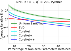
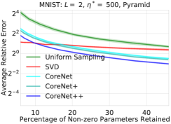
Refer to caption
Refer to caption
Refer to caption
Refer to caption
Refer to caption
Refer to caption
Refer to caption
Refer to caption
Refer to caption
Refer to caption
Refer to caption
Refer to caption
Refer to caption
Refer to caption
Refer to caption
Figure 3: Evaluations against the MNIST dataset with varying number of hidden layers (L𝐿L) and number of neurons per hidden layer (ηsuperscript𝜂\eta^{*}). Shaded region corresponds to values within one standard deviation of the mean. The figures show that our algorithm’s relative performance increases as the number of layers (and hence the number of redundant parameters) increases.
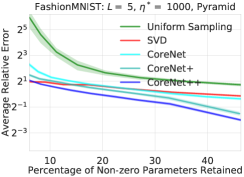
Refer to caption
Refer to caption
Refer to caption
Refer to caption
Refer to caption
Refer to caption
Refer to caption
Refer to caption
Refer to caption
Refer to caption
Refer to caption
Refer to caption
Refer to caption
Refer to caption
Refer to caption
Figure 4: Evaluations against the CIFAR-10 dataset with varying number of hidden layers (L𝐿L) and number of neurons per hidden layer (ηsuperscript𝜂\eta^{*}). The trend of our algorithm’s improved relative performance as the number of parameters increases (previously depicted in Fig. 3) also holds for the CIFAR-10 data set.
Refer to caption
Refer to caption
Refer to caption
Refer to caption
Refer to caption
Refer to caption
Refer to caption
Refer to caption
Refer to caption
Refer to caption
Refer to caption
Refer to caption
Refer to caption
Refer to caption
Refer to caption
Figure 5: Evaluations against the FashionMNIST dataset with varying number of hidden layers (L𝐿L) and number of neurons per hidden layer (ηsuperscript𝜂\eta^{*}).
Refer to caption
Refer to caption
Refer to caption
Refer to caption
Refer to caption
Refer to caption
Refer to caption
Refer to caption
Refer to caption
Refer to caption
Refer to caption
Refer to caption
Refer to caption
Refer to caption
Refer to caption
Figure 6: Evaluations against the MNIST dataset with varying number of hidden layers (L𝐿L) and number of neurons per hidden layer (ηsuperscript𝜂\eta^{*}). Shaded region corresponds to values within one standard deviation of the mean. The figures show that our algorithm’s relative performance increases as the number of layers (and hence the number of redundant parameters) increases.
Refer to caption
Refer to caption
Refer to caption
Refer to caption
Refer to caption
Refer to caption
Refer to caption
Refer to caption
Refer to caption
Refer to caption
Refer to caption
Refer to caption
Refer to caption
Refer to caption
Refer to caption
Figure 7: Evaluations against the CIFAR-10 dataset with varying number of hidden layers (L𝐿L) and number of neurons per hidden layer (ηsuperscript𝜂\eta^{*}). The trend of our algorithm’s improved relative performance as the number of parameters increases (previously depicted in Fig. 6) also holds for the CIFAR-10 data set.
Refer to caption
Refer to caption
Refer to caption
Refer to caption
Refer to caption
Refer to caption
Refer to caption
Refer to caption
Refer to caption
Refer to caption
Refer to caption
Refer to caption
Refer to caption
Refer to caption
Refer to caption
Figure 8: Evaluations against the FashionMNIST dataset with varying number of hidden layers (L𝐿L) and number of neurons per hidden layer (ηsuperscript𝜂\eta^{*}).