Abundance of peaks and dips in three-dimensional mass and halo density fields: a test for cosmology

Abstract

Using cosmological N-body simulations, we study the abundance of local maxima (peaks) and minima (dips) identified in the smoothed distribution of halos and dark matter (DM) on scales of $10-100$s Mpcs. The simulations include Gaussian and local-type $f_{{}_{\rm NL}}$ non-Gaussian initial conditions. The expression derived in the literature for the abundance (irrespective of height) of peaks for Gaussian fields is surprisingly accurate for the evolved halo and DM density fields for all initial conditions considered. Furthermore, the height distribution is very well fitted by a log-normal on quasi-linear scales. The abundance as a function of scale depends on the cosmological parameters ($H_{0}$ and background matter densities) through the shape of the power spectrum, but it is insensitive to the clustering amplitude. Further, the abundance in the smoothed halo distribution is substantially different in the non-Gaussian from the Gaussian simulations. The interpretation of this effect is straightforward in terms of the scale dependence of halo bias in non-Gaussian models. The abundance of extrema extracted from three-dimensional large galaxy redshift surveys could be a competitive probe of the cosmological parameters and initial non-Gaussianity. It breaks the degeneracy between $f_{{}_{\rm NL}}$ and the clustering amplitude, making it complementary to counts of galaxy clusters and peaks in weak-lensing maps.

1 Introduction

Peaks in the underlying mass density field are the most likely sites for the formation of halos where gas is expected to accrete and form galaxies (White & Rees, 1978). In the classical picture of Press & Schechter (1974), matter in regions with linear density contrast above a threshold $\delta_{c}$ is assigned to halos of mass larger than $M$, where $M$ defines the smoothing of the density field. This implies that halos of mass $M$ form at peaks with $\delta=\delta_{c}$ in the smoothed density contrast $\delta$.

Naturally, most studies have focused on peaks associated with halos. Indeed, statistical properties of local extrema (e.g. Adler, 1981) have gained a great deal of attention in cosmology (Bardeen et al., 1986) (hereafter BBKS). Correlations of halos and their distribution in relation to the mass density field of the gravitationally dominant dark matter (DM), i.e. biasing (Kaiser & N., 1984), have been studied extensively with analytic methods and numerical simulations. For Gaussian initial conditions and on sufficiently large scales, halos follow a linear biasing relation, $\delta_{\mathrm{h}}=b\delta$ between the halo number density contrast, $\delta_{\mathrm{h}}$ and the mass density contrast $\delta$. The bias factor $b$ depends on the height of the peaks associated with halos and on their mass. An important result obtained in simulations (Dalal et al., 2008), and confirmed by analytic techniques (Grinstein & Wise, 1986; Dalal et al., 2008; Matarrese & Verde, 2008; Slosar et al., 2008), is that the presence of initial local-type non-Gaussianity introduces a peculiar scale dependence in the bias factor dubbed “non-Gaussian bias”. The specific form of $b(k)$ ($k$ is the wavenumber of a given scale) opens the window for probing initial non-Gaussianity based on the clustering properties of galaxies in planned large redshift surveys, e.g. Euclid (Laureijs et al., 2011) and DESI (DESI Collaboration et al., 2016).

It is well known that non-Gaussianity strongly affects the tails of density probability distributions (Adler, 1981; Catelan et al., 1988a). Several authors have further specialized these results to local density maxima of non-Gaussian density fields, where the non-Gaussianity is either of a generic form (e.g. Catelan et al., 1988b; Gay et al., 2012; Codis et al., 2013; Uhlemann et al., 2018) or developed via non-linear gravitational evolution of initial gaussian conditions (e.g. Suginohara, 1991; Matsubara, 1994). In particular, Gay et al. (2012); Codis et al. (2013) considered the effect of a generic non-Gaussianity on extrema counts and Minkowski functionals of the dark matter density field. In this work, we consider peaks and dips in cosmological density field smoothed on scales much larger than those of galactic and galaxy cluster halos ($\lower 2.15277pt\hbox{$\;\buildrel<\over{\sim}\;$}10$ Mpcs). Using N-body simulations in large cosmological boxes, we focus on the total number of local extrema for density fields constructed from the halo distribution, as a proxy for a galaxy catalogue. Earlier analyses (Croft & Gaztanaga (1998); De & Croft (2007, 2010)) have used this type of statistics for constraining parameters related to the linear matter power spectrum on smaller scales ($\lower 2.15277pt\hbox{$\;\buildrel<\over{\sim}\;$}10$ Mpcs). Our goal is to assess the extent to which the abundance of extrema in three-dimensional (3D) fields inferred from current and forthcoming large galaxy redshift surveys can be used as a cosmological tool and, more specifically, a probe of local primordial non-Gaussianity. As we shall see, our main findings have a straightforward interpretation in terms of the non-Gaussian bias.

We adopt standard notation. The mean total and baryonic mass densities (in units of the critical density) are denoted by $\Omega_{\mathrm{m}}$ and $\Omega_{\mathrm{b}}$, respectively. The Hubble constant is $H_{0}$ and $h=H_{0}/[100\mathrm{\,{\rm km}\,{\rm s}^{-1}\;Mpc^{-1}}]$. The linear growth factor (normalized to unity at the present time) at redshift, $z$, is $D(z)$. The outline of the paper is as follows. In §2 we lay out known relations between the number of extrema and the underlying power spectrum for Gaussian fields. A description of the N-body simulations is provided in §3 and the corresponding results for the abundance of local extrema identified in smoothed density fields derived from the DM and halo distributions are in §4. In §5 we discuss the prospects for the application of the number of extrema as a test of cosmological parameters and conclude with a summary in §6.

2 Definitions and Theoretical Expectations

We define local maxima (peaks) in a smoothed random field, $f$, as points in space where the spatial gradient is $\partial_{\alpha}f=0$ and the Hessian $\partial_{\alpha}\partial_{\beta}f$ is negative definite. Local minima (dips) are defined similarly but with a positive definite Hessian. For a random Gaussian field, peaks and dips have an equal total number per unit volume, which was computed by BBKS to be

$$n_{0}\approx 0.016R_{*}^{-3}\;,$$ (1)

where

$$R_{*}=\sqrt{3}{\textstyle{\sigma_{1}\over\sigma_{2}}}\;,$$ (2)

and the spectral moments

$$\sigma^{2}_{j}=\int{\textstyle{k^{2}\textrm{d}k\over 2\pi^{2}}}P(k)W_{R}^{2}(k)k^{2j}\;.$$ (3)

The expression for $n_{0}$ is independent of the clustering amplitude and it depends only on the shape of the power spectrum, $P(k)$ of the field, and the smoothing Kernel $W_{R}(k)$. For $P(k)\sim k^{n}$, and a Gaussian smoothing window $W_{R}^{2}(k)=\exp(-k^{2}R^{2})$, it is easy to see that,

$${\textstyle{R\over R_{*}}}=\left({\textstyle{n+5\over 6}}\right)^{1/2}\;.$$ (4)

The total number of peaks is preserved under a local monotonous one-to-one mapping, $F(\delta)$, of the density field. Thus we expect this quantity to be independent of time in the quasi-linear scales. On smaller scales, local extrema tend to merge and diffuse, leading to deviations from expression Eq. (1) above.

In addition to the DM density field, we also examine peaks and dips in the smoothed distribution of halos. The corresponding spectral moments $\sigma_{j}\equiv\sigma_{j,h}$ are given by

$$\sigma_{j,h}^{2}=\int{\textstyle{k^{2}dk\over 2\pi^{2}}}\,k^{2j}W_{R}^{2}(k)\Big{[}b^{2}(k)P(k)+{\textstyle{1\over\bar{n}_{h}}}\Big{]}\;.$$ (5)

The expression in square brackets is a model for the power spectrum of the halo distribution where $P(k)$ here refers to the underlying density field and $b(k)$ describes the scale-dependent halo bias. The term $1/{\bar{n}_{h}}$ is due to the finite number of halos and approximated as a Poisson discreteness noise. Using the simulations described below we have found that the added discreteness variance is strongly suppressed for large smoothing and is actually sub-Poissonian, in agreement with the findings of Casas-Miranda et al. (2002); Hamaus et al. (2010). On linear scales, the halo bias $b(k)$ is constant for Gaussian initial conditions but depends on the halo mass i.e. $b(k)=b^{\mathrm{G}}(M)$.

We also consider local-type non-Gaussianity (Salopek & Bond, 1990; Gangui et al., 1993; Komatsu & Spergel, 2001) for which the Bardeen potential $\Phi$ deep in matter domination is expanded around a random Gaussian field $\phi$ as

$$\Phi(\mathbf{x})=\phi(\mathbf{x})+f_{\rm NL}\left(\left[\phi(\mathbf{x})\right]^{2}-\langle\phi^{2}\rangle\right)\;.$$ (6)

The bispectrum of $\Phi$ induces the following scale dependence in the bias factor,

$$b(k)=b^{\mathrm{G}}(M)+{\textstyle{\alpha(f_{{}_{\rm NL}})\over k^{2}T(k)}}\;,$$ (7)

where

$$\alpha(f_{{}_{\rm NL}})\equiv 3f_{{}_{\rm NL}}{\textstyle{\partial{\rm ln}\,\bar{n}_{h}\over\partial{\rm ln}\,\sigma_{8}}}{\textstyle{\Omega_{m}H_{0}^{2}\over D(z)c^{2}}}\;,$$ (8)

and $\bar{n}_{h}(M)$ is the abundance of halos (per unit $M$) computed for the Gaussian field without the $f_{{}_{\rm NL}}$ terms. When implementing Eq. (5) to compare it to data (see Section §4), we use the following approximation

$${\textstyle{\partial{\rm ln}\,\bar{n}_{h}\over\partial{\rm ln}\,\sigma_{8}}}\approx\delta_{c}(b^{\rm G}(M)-1),$$ (9)

with $\delta_{c}=1.687$, which is valid for universal mass functions and the spherical collapse model . We do not include expressions (e.g. Gay et al., 2012) for the theoretical corrections to Eq. (1) due to $f_{{}_{\rm NL}}$ non-Gaussianity. Indeed, we will see below that the expression remains accurate provided that the appropriate $\sigma_{i}$ is used.

3 Simulations

Two sets of simulations, respectively in a $2h^{-1}\,{\rm Gpc}$ and a $3h^{-1}\,{\rm Gpc}$ box, are available for initial conditions generated from $\Lambda$CDM initial power spectra with slightly different cosmological parameters, as described in the Table. The simulations were run with the Gadget2 (Springel, 2005) N-body code on the Baobab cluster at the University of Geneva. The initial particle displacements were implemented at $z_{i}=99$ using the public code 2LPTic (Crocce et al., 2006) for realizations with Gaussian initial conditions and its modified version (Scoccimarro et al., 2012) for non-Gaussian initial conditions of the local type. The transfer function for the smaller box (simulations 1, see Table) was obtained using the CLASS code (Blas et al., 2011). This set contains runs for Gaussian initial conditions and two for local-type non-Gaussianity respectively, with $f_{{}_{\rm NL}}=250$ and $f_{{}_{\rm NL}}=-250$. For each of these initial conditions, we obtain 8 random realizations corresponding to different random seeds.

The transfer function of the second set, simulations 2, was obtained using the CAMB code (Lewis et al., 2000). This set includes 3 types of models: Gaussian initial conditions ($f_{{}_{\rm NL}}=0$) and non-Gaussian initial conditions, respectively, with $f_{{}_{\rm NL}}=100$ and $f_{{}_{\rm NL}}=-100$. For each type of models, we have 3 simulations corresponding to different random realizations of the initial conditions. The Rockstar (Behroozi et al., 2013) algorithm is employed to identify halos, with linking length $\lambda=0.28$.

	$L$	$N_{\mathrm{p}}$	$M_{\mathrm{halo}}$	$\sigma_{8}$	$\Omega_{m}$	$\Omega_{b}$
sim 1	2	$1536^{3}$	$3.67$	0.85	0.3	0.0455
sim 2	3	$1024^{3}$	$37.9$	0.81	0.272	0.0455

Table 1: Simulation parameters, where $L$ is the box size (in unit of $h^{-1}\,{\rm Gpc}$), $N_{\mathrm{p}}$ number of simulation particles, and $M_{\mathrm{halo}}$ is the minimum halo mass identified in the simulation (in unit of $10^{12}h^{-1}{\rm M}_{\odot}$). Both, simulations 1&2, include Gaussian and two choices for non-Gaussian initial conditions. Outputs of simulations 1 are available at $z=0$ and $z=1$, while only the output at $z=0$ is available for simulations 2. In all simulations the Hubble parameter is $h=0.7$ and the spectral index of the initial power spectrum at large scales is $n_{s}=0.967$.

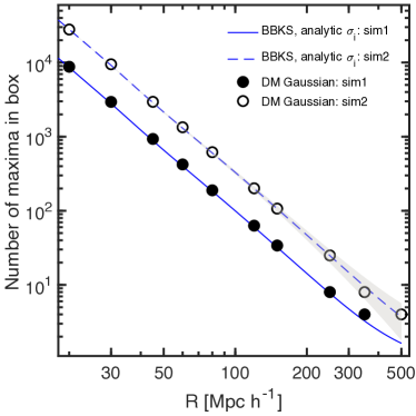
Density fields are interpolated from the DM and halo distributions in the simulation box on a $512^{3}$ cubic grid using the Clouds-in-Cells (CIC) scheme. The grid spacing is thus $3.9h^{-1}\,{\rm Mpc}$ and $5.85h^{-1}\,{\rm Mpc}$, for simulations 1 & 2, respectively. The density fields were additionally smoothed with a Gaussian window of 8 different widths in the range $20h^{-1}\,{\rm Mpc}$ to $500h^{-1}\,{\rm Mpc}$. For each smoothed field, local maxima (minima) were identified as grid points surrounded by grid points with lower (higher) density values. Fig. 1 shows the total number of maxima in the smoothed DM density field in the full boxes of simulations 1 & 2 at $z=0$. The theoretical predictions obtained from the BBKS expression (Eqs. 1-2) using the linear power spectrum $P(k)=P_{\mathrm{L}}(k)$ for the two models are also shown, as indicated in the figure. The shaded area encompasses the expected range of (1$\sigma$) shot-noise for simulations 2. The number drops like $R^{-3}$, consistently with Eq. (1) since $R_{*}\propto R$ upto a factor of $\mathcal{O}(1)$ which depends on the shape of the power spectrum at scale $R$ (cf. Eq. 4). The figure refers to the Gaussian simulations only. A similar figure can be found in (Ludlow & Porciani, 2011), but for comparison of the theoretical expression with peaks identified in the initial conditions of their simulations.

Figure 1: Total number of maxima versus the smoothing length, from the DM distribution in simulations 1 & 2 for Gaussian initial conditions at redshift $z=0$ The lines represent the corresponding theoretical prediction using eq. 1 and the shaded area represents the $1\sigma$ shot-noise for the larger simulation.

4 Results

4.1 Total number of minima and maxima

Gaussian initial conditions imply equal probability of producing peaks and dips, up-to fluctuations due to the finite box size. However, on scales $\lower 2.15277pt\hbox{$\;\buildrel<\over{\sim}\;$}10$s of Mpcs, non-linear gravitational evolution breaks the initial symmetry through the merging and smearing of dips and peaks. For non-Gaussian initial conditions, the statistical symmetry between maxima and minima is already broken initially.

We choose to first analyze the (total) number $n_{\mathrm{1}}$, per unit volume, of minima, $n_{\mathrm{min}}$, and maxima, $n_{\mathrm{max}}$ in the simulations. The differences between the abundance of minima and maxima will be discussed at a later stage. More precisely, we consider

$$n_{\mathrm{1}}={\textstyle{1\over 2}}\big{(}n_{\mathrm{min}}+n_{\mathrm{max}}\big{)}\;,$$ (10)

which is computed from the smoothed density fields for the various simulations. An advantage of $n_{1}$ is that it boosts the statistical significance of the measured abundance. For a Gaussian field, $n_{1}=n_{0}$ given in Eq. (1). Inclusion of non-Gaussian terms modify the abundance of either the minima or maxima by a leading-order correction proportional to the skewness of the density field and its derivatives (Gay et al., 2012). The combined leading order correction for both minima and maxima cancel out in the expression of $n_{\mathrm{1}}$. Consequently, the BBKS prediction Eq. (1) remains valid up to a small correction of order $f_{{}_{\rm NL}}^{2}$.

According to Fig. 1, differences in $n_{1}$ between the simulations are visually hard to examine directly. Thus, we consider the statistic,

$$\Upsilon\equiv{\textstyle{n_{1}R^{3}\over 0.016}}$$ (11)

where $R$ is the width of the smoothing window. According to Eq. (1), for a Gaussian field $\Upsilon=({R}/{R_{*}})^{3}$. The three-panel Fig. 2 summarizes the main results. The top panel plots $\Upsilon$, averaged over the 8 random realizations in simulations 1, against the smoothing length, $R$, for the DM density field. The shaded area represents the 1$\sigma$ shot-noise in $n_{1}$ corresponding to the finite number of peaks and dips in the simulation box. It is estimated as $\sqrt{n_{0}L^{3}/2}$ where $n_{0}$ is the theoretical value according to Eq. (1) and the factor of $1/2$ arises from the definition of $n_{1}$ which involves both minima and maxima. We have checked that the scatter from the 8 individual runs (not shown for clarity) is consistent with this estimate of the shot-noise. For our Gaussian as well as non-Gaussian simulations, the results in the top panel for $z=1$ and $z=0$ are almost identical. The dotted line shows $(R/R_{*})^{3}$ computed according to the theoretical expression Eq. (2) derived for Gaussian fields, where $\sigma_{i}$ are computed using Eq. (3) with the initial power spectrum $P_{\mathrm{L}}(k)$. There is a reasonable match between the dotted curve and $(R/R_{*})^{3}$ derived from $n_{1}$ for the Gaussian simulations (black and red solid curves). Overall, the impact of $f_{{}_{\rm NL}}$ is very small, in agreement with the fact that, for dark matter, $n_{1}$ depends on $f_{{}_{\rm NL}}$ only at order $f_{{}_{\rm NL}}^{2}$.

The middle panel refers to results obtained from the halo distribution in simulations 1. The solid curves corresponding to the Gaussian simulations at $z=1$ and $z=0$ are similar. In great contrast to the upper panel, both $f_{{}_{\rm NL}}=250$ and $f_{{}_{\rm NL}}=-250$ models (dashed and dash-dotted lines) at the two redshifts are substantially different. It is interesting to check how well the BBKS expression in Eq. (2) fits the $\Upsilon$ computed from the halos in the non-Gaussian simulations. To do that we compute $(R/R_{*})^{3}$ using Eq. (2) for $\sigma_{1}$ and $\sigma_{2}$ computed directly from the halo density fields. The results are plotted as the plus signs and circles, respectively, for the $f_{{}_{\rm NL}}=250$ and $f_{{}_{\rm NL}}=-250$ simulations. We present the $z=1$ case only but the excellent agreement of $\Upsilon$ with $(R/R_{*})^{3}$ computed from $n_{\mathrm{1}}$ also holds at $z=0$ . The bottom panel summarizes results for simulations 2 ($z=0$) of the larger box. The halos in these simulations have a larger mass and therefore follow a different biasing relation than halos in simulations 1, yielding different quantitative results. For these simulations also, the BBKS expression (computed with $\sigma_{i}$ measured in the simulations), shown as the plus signs and circles, furnishes an excellent match. Therefore, despite the fact that relations Eqs. (1) and (2) are formally obtained for Gaussian fields, they remain accurate for the non-Gaussian fields considered here, provided the actual $\sigma_{i}$ are used.

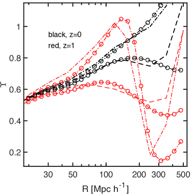
In Fig. 3 we compare the theoretical expectation of Eq. (5) against $\Upsilon$ measured from the non-Gaussian simulations. The theoretical curve fits good the data on scales $R\lesssim 100$Mpc/h and provides a qualitatively good description at all scales. Deviations may be due in part to our approximation Eq. (9) and, especially at large scales, to the finite box size of the simulations.

Figure 2: The quantity $\Upsilon$ as estimated from Eq. (11). Top: from the number of peaks and throughs in the dark matter distribution of simulations 1. Middle: The same the Top, but for the halo distribution. Bottom: For DM and halos for simulations 2, at $z=0$ only. In all panels, the grey area represents the shot-noise estimated from the expression with using the theoretical linear power spectrum.

Figure 3: A test of the analytic prediction for the non-Gaussian model. The dashed and dash-dotted curves are taken from the middle panel in the previous figure. The curves with the circles plot $(R/R_{*})^{3}$ computed with the approximate $\sigma_{i}$ given in Eqs. (5-7)

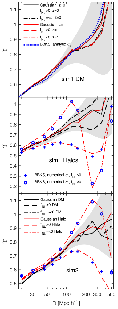
To conclude this Section, we note that the effect of $f_{{}_{\rm NL}}$ on $\Upsilon$ is only weakly degenerate with that of $\sigma_{8}$ because $n_{1}$ primarily depends on the ratio of spectral moments $\sigma_{1,h}/\sigma_{2,h}$.

4.2 Asymmetry and height distribution

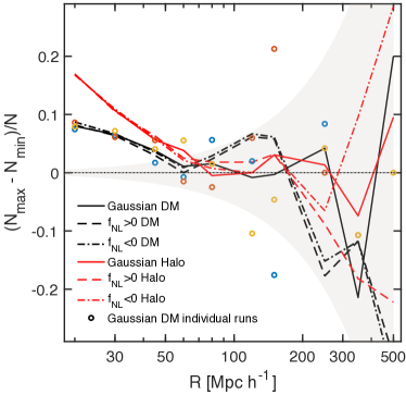
So far we have considered $n_{1}$, without distinguishing between minima and maxima. In Fig. 4, we examine the asymmetry between the abundances of minima and maxima as a function of the smoothing width for simulations 2 at redshift $z=0$. There is a clear excess of $N_{\mathrm{max}}$, which is significantly above the level of the shot-noise (grey area). The trend is reversed at larger scales for both DM non-Gaussian models, but it becomes immersed in the shot-noise. Results of the three individual runs for the Gaussian DM simulation are also shown. It is clear that the shot-noise estimated theoretically as described above (grey area) is consistent with the scatter in the individual runs.

We explore the probability density distribution (PDF) of the value of the densities at the minima and maxima. We define,

$$\nu={\textstyle{\delta\over\sigma_{0}}}\quad{\rm and}\quad\nu_{\mathrm{ln}}={\textstyle{{\rm ln}\,(1+\delta)-\mu\over\sigma_{\mathrm{ln}}}}$$ (12)

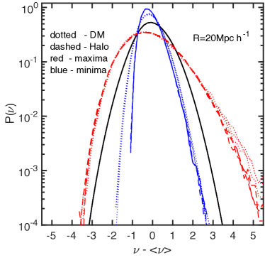
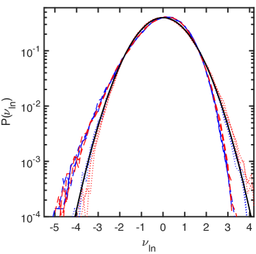
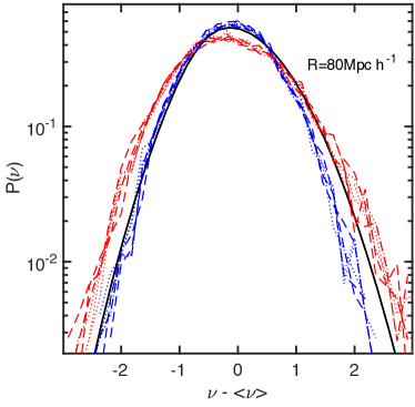
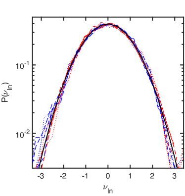
where $\sigma_{0}$ is the rms of density field all over space while $\mu$ and $\sigma_{\mathrm{ln}}$ are the mean and rms of the values of ${\rm ln}\,(1+\delta)$ at either the minima or maxima. The quantity $\nu_{\mathrm{ln}}$ is motivated by the result that the PDF of the density field is well approximated by a log-normal distribution (e.g. Coles & Jones, 1991; Kofman et al., 1994). In Fig. 5 and 6 we plot the PDF of $\nu$ (top) and $\nu_{\mathrm{ln}}$ (bottom) for a smoothing of $R=20h^{-1}\,{\rm Mpc}$ and $80h^{-1}\,{\rm Mpc}$ for simulations 2. The 3 curves of each line-style correspond to the Gaussian and 2 non-Gaussian simulations. It is evident that the PDF of densities at either maxima or minima is weakly sensitive to whether the initial conditions were Gaussian or not. This is expected given that corrections arise at order $f_{\rm NL}^{2}$ as noted above. Thus, for clarity, the plot does not indicate which of the simulations is shown. For $R=20h^{-1}\,{\rm Mpc}$, the BBKS theoretical prediction for $P(\nu)$ (expression 4.3 in their paper) shown as the black in the top panel, is a poor fit to any of the PDFs measured in the simulations. However, $P(\nu_{\mathrm{ln}})$ for the DM density field (dotted), exhibit only minor differences at the tails, where the PDF for maxima is slightly skewed to positive values relative to the Gaussian (black in the bottom panel), the distribution at minima is negatively skewed. The rather small differences between the PDF from the halos and the corresponding DM are due to deviations from linear biasing. Fig. 6 shows the same results, but for $R=80h^{-1}\,{\rm Mpc}$. This large smoothing greatly reduces the effect of non-linear evolution, bringing the BBKS theoretical PDF (black curve, top panels) closer to the measured PDF than it is for $R=20h^{-1}\,{\rm Mpc}$. The log-normal curve (black, bottom) remains a good fit to $P(\nu_{\mathrm{ln}}$ for the DM although not as good as in the smaller smoothing. It is interesting that the log-normal describes the halo PDF fairly well for this smoothing. At $R=20h^{-1}\,{\rm Mpc}$ and $80h^{-1}\,{\rm Mpc}$ the halo bias in the Gaussian and non-Gaussian simulations are small (cf. Eq. (7). This explains the similarity between the halo PDFs in the simulations irrespective of the initial statistic.

Figure 4: The relative difference between the total number of maxima and minima in simulations 2, versus the smoothing width, at redshift $z=0$.

Figure 5: Top: The PDF of $\nu$ at minima and maxima in simulations 2, as indicated in the figure. The black curve is the theoretical prediction for $P(\nu)$ given in BBKS. Bottom: The PDF of $\nu_{\mathrm{ln}}$ at minima and maxima for simulations 2. Here the black line is a Gaussian with zero mean and unit variance.

Figure 6: The same as the previous figure, but for $R=80h^{-1}\,{\rm Mpc}$.

5 Abundance of extrema as a cosmological test

We offer a preliminary assessment of using total number of peaks and dips as a test of cosmological models. A proper analysis should take into account the covariance between the abundances corresponding to different smoothing scales. However, this task is beyond the scope of the current paper. Instead, we will focus on the expected discriminatory power of extrema abundance at distinct scales. As an example, we consider the Euclid mission (Laureijs et al., 2011), which will target emision line galaxies in the redfshift range $0.9<z<1.8$ across $\sim 35\%$ of the sky. For Planck’s cosmological parameters, the corresponding survey volume is $48(h^{-1}\,{\rm Gpc})^{3}$. Furthermore, the typical host halo mass is $\sim 10^{11-12}h^{-1}{\rm M}_{\odot}$, in broad agreement with the minimum halo mass resolved in simulations 1.

We wish to assess the ability that a measured total number $N$ of extrema in a survey can reject a certain model given the hypothesis of an assumed fiducial underlying model. For this purpose, we assume that $N$ follows a Poisson distribution

$$P_{\bar{N}}(N)={\textstyle{{\bar{N}}^{N}\over N!}}\mathrm{e}^{-\bar{N}}\;,$$ (13)

where $\bar{N}$ is the mean number expected in a particular given model. Given an observed $N$, the preferred of two competing models with expected mean numbers ${\bar{N}}_{1}$ and ${\bar{N}}_{2}$, respectively, is determined by

$$D_{{}_{\bar{N}_{1}\bar{N}_{2}}} = -2{\rm ln}\,{\textstyle{P_{{\bar{N}}_{1}}\over P_{{\bar{N}}_{2}}}}$$ (14)

$$= 2N{\rm ln}\,{\textstyle{\bar{N}_{2}\over\bar{N}_{1}}}+2({\bar{N}_{1}-\bar{N}_{2}})\;.$$

The mean value of $D$ over all measurements, which we loosely denote by $\Delta\chi^{2}$ is

$$\Delta\chi^{2} = \sum_{N}P_{\bar{N}}D_{{}_{\bar{N}_{1}\bar{N}_{2}}}$$ (15)

$$= 2\bar{N}{\rm ln}\,{\textstyle{\bar{N}_{2}\over\bar{N}_{1}}}+2({\bar{N}_{1}-\bar{N}_{2}})\;,$$

where we have used $\sum_{N}P_{\bar{N}}(N)=1$ and $\sum_{N}NP_{\bar{N}}(N)=\bar{N}$. For $\bar{N}_{2}=\bar{N}$, the quantity $\Delta\chi^{2}$ yields the confidence level with which a model with $\bar{N}_{1}$ can be rejected if the underlying model is $\bar{N}$. We use this statistic to assess whether the abundance of dips and peaks can be used to reject certain models given a Gaussian cosmological model with fiducial cosmological parameter. We focus on $\Omega_{m}$ and $f_{{}_{\rm NL}}$, separately.

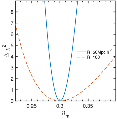
Fig. 7 examines $\Delta\chi^{2}$ as a function of the matter density $\Omega_{\mathrm{m}}$. Here, $\bar{N}$ is computed using Eq. (1-3) for fiducial DM linear power spectrum with the cosmological parameters corresponding to simulations 1. The same parameters with the exception of $\Omega_{\mathrm{m}}$ are used in the same expression to derive $\bar{N}_{1}$. This figure, therefore, refers to a Gaussian model ($f_{{}_{\rm NL}}=0$) and, in addition to DM density fields, it is also relevant for halos with linear constant bias with respect to the DM. Only two filtering scales are considered, as indicated in the figure. It is remarkable that for $R=50h^{-1}\,{\rm Mpc}$ the $1\sigma$ level ($\Delta\chi^{2}=1$) is at $\Delta\Omega\approx\pm 0.01$ from the fiducial $\Omega_{m}=0.3$. It should be pointed out that for the $\Lambda$CDM linear power spectrum the abundance on a filtering scale given in $h^{-1}\,{\rm Mpc}$ is degenerate with respect to $\Omega_{m}h$ and $\Omega_{b}h$. This sensitivity to $\Omega_{m}$ declines rapidly at $R=100h^{-1}\,{\rm Mpc}$ due to the $1/R^{3}$ dependence of the number of dips and peaks.

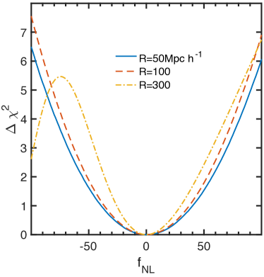
The sensitivity to $f_{{}_{\rm NL}}$ is demonstrated in Fig. 8 plotting $\Delta\chi^{2}$ with $\bar{N}$ from the fiducial model and $\bar{N}_{1}$ for $f_{{}_{\rm NL}}\neq 0$ but with all other parameters fixed at the fiducial values. These curves refer to filtered halo distribution where the theoretical expressions in Eqs. (5-7) are used in Eq. (1) to derive the mean number of dips and peaks $\bar{N}$ in a Euclid volume survey at $z=1$. In these calculations, we consider a halo mass distribution consistent with simulations 1, with a minimum mass of $3.67\times 10^{12}h^{-1}M_{\odot}$. For this mass threshold, we have seen in the previous section that the theoretical predictions are in reasonable agreement with the simulations. The sensitivity to $f_{{}_{\rm NL}}$ is improved for the larger filtering widths, $R$ thanks to the stronger $f_{{}_{\rm NL}}$-dependence of halo bias on larger scales. For $R=300h^{-1}\,{\rm Mpc}$, we find $\Delta\chi^{2}=1$ for deviations $\Delta f_{{}_{\rm NL}}\approx\pm 25$. This is encouraging especially if combined with measurements as a function of filtering scales and different halo masses.

Figure 7: Abundance of dips and peaks as a cosmological test for estimating $\Omega_{\mathrm{m}}$ from a survey like Euclid. Values of $\Delta\chi^{2}=1$ correspond to $1\sigma$ limits from the fiducial value of $\Omega_{\mathrm{m}}$.

Figure 8: The same as the previous figure but for $f_{{}_{\rm NL}}$ instead of $\Omega_{\mathrm{m}}$.

6 Discussion and Conclusions

Locating points of maxima and minima is straightforward even for 3D density fields estimated from realistic galaxy redshift surveys. Since the total abundance is computed irrespective of height, it should be robust against the details of how the density field is estimated from the data. The total abundance is also insensitive to redshift space distortions, which in any case can be modeled with standard perturbation theory for smoothing widths $R\gtrsim 50h^{-1}\,{\rm Mpc}$ (Codis et al., 2013) (see also Lam et al., 2010). Further, it depends explicitly only on the shape of the power spectrum. Any dependence on the amplitude (e.g. $\sigma_{8}$) is indirectly encoded in non-linear corrections to the shape of the gravitationally evolved power spectrum. The lack of sensitivity of this abundance statistics on the amplitude thereby implies that it breaks most of the degeneracy between $f_{{}_{\rm NL}}$ and the primordial amplitude of scalar perturbations, which arises in measurements of galaxy clusters counts and shear peaks in weak lensing maps for instance (this degeneracy can also be broken by combining clusters and voids, see Kamionkowski et al., 2009). We have demonstrated that a primordial non-Gaussianity of the local-$f_{{}_{\rm NL}}$ type imprints a strong signal in the abundance of peaks and dips of the halo density field owing to the non-Gaussian bias. An important result of the current paper is that the BBKS prediction derived for Gaussian density field can account for this effect reasonably well, provided that the matter power spectrum is replaced by the halo power spectrum. Therefore, the abundance of peaks and dips (a 1-point statistics) is sensitive to the scale-dependent bias in the halo power spectrum (a 2-point statistics), like the covariance of cluster counts (Cunha et al., 2010). This effect disappears when the density field perfectly traces the matter distribution as is the case for shear peaks for instance.

We have made a preliminary assessment of the applicability of the total abundance statistics as a test of $f_{{}_{\rm NL}}$ for a survey with specifications similar to those of the Euclid mission (Laureijs et al., 2011). From a measurement at a single smoothing scale $R$, we obtain an uncertainty of $\Delta f_{{}_{\rm NL}}=25$ (for $R=300h^{-1}\,{\rm Mpc}$) and 40 (for $R=50h^{-1}\,{\rm Mpc}$). This suggests that a measurement combining different smoothing scales and halo masses should be able to achieve a sensitivity of $\Delta f_{{}_{\rm NL}}\lesssim 10$. While the sensitivity of this approach will likely be worse than the limits set by the latest CMB measurements from Planck, $f_{{}_{\rm NL}}=0.8\pm 5$ (Planck Collaboration et al., 2016), this approach should be competitive with galaxy clusters and shear peak counts in weak-lensing maps, for which the forecasted uncertainty is $\Delta f_{{}_{\rm NL}}\sim 9$ (e.g. Pillepich et al., 2012, for a galaxy survey like eROSITA) and $\Delta f_{{}_{\rm NL}}\sim 13$ (e.g., Marian et al., 2011, for a weak-lensing survey with Euclid specifications), respectively. However, our approach may also be affected by the Eddington bias that plagues galaxy cluster counts or shear peaks. Namely, additive noise in the data will presumably increase the number of peaks while reducing the number of dips, which would mimic a small positive $f_{{}_{\rm NL}}$. We will defer a more detailed study of this effect to future work.

The abundance of extrema depends on the cosmological parameters of the background cosmology. Here we explored the dependence on $\Omega_{m}$ alone with very encouraging results of an accuracy at the level of $\Delta\Omega_{\mathrm{m}}\sim 0.01$. For a given filtering scale given in $h^{-1}\,{\rm Mpc}$, the abundance depends is nearly degenerate with the combination $\Omega_{\mathrm{m}}h$. Thus, this result regarding $\Omega_{\mathrm{m}}$ could alternatively by expressed as an accuracy of $0.7\,{\rm km}\,{\rm s}^{-1}$ on $H_{0}$ if all other parameters are fixed.

References

- Adler (1981) Adler R. J., 1981, The Geometry of Random Fields. Chichester: Wiley, doi:10.1137/1.9780898718980
- Bardeen et al. (1986) Bardeen J. M., Bond J. R., Kaiser N., Szalay A. S., 1986, ApJ, 304, 15
- Behroozi et al. (2013) Behroozi P. S., Wechsler R. H., Wu H. Y., 2013, ApJ, 762
- Biagetti et al. (2017) Biagetti M., Lazeyras T., Baldauf T., Desjacques V., Schmidt F., 2017, Mon. Not. Roy. Astron. Soc., 468, 3277
- Blas et al. (2011) Blas D., Lesgourgues J., Tram T., 2011, JCAP, 2011
- Casas-Miranda et al. (2002) Casas-Miranda R., Mo H. J., Sheth R. K., Boerner G., 2002, MNRAS, 333, 730
- Catelan et al. (1988a) Catelan P., Lucchin F., Matarrese S., 1988a, Physical Review Letters, 61, 267
- Catelan et al. (1988b) Catelan P., Lucchin F., Matarrese S., 1988b, PRL, 61, 267
- Codis et al. (2013) Codis S., Pichon C., Pogosyan D., Bernardeau F., Matsubara T., 2013, MNRAS, 435, 531
- Coles & Jones (1991) Coles P., Jones B., 1991, MNRAS, 248, 1
- Crocce et al. (2006) Crocce M., Pueblas S., Scoccimarro R., 2006, MNRAS, 373, 369
- Croft & Gaztanaga (1998) Croft R. A. C., Gaztanaga E., 1998, Astrophys. J., 495, 554
- Cunha et al. (2010) Cunha C., Huterer D., Doré O., 2010, Phys. Rev. D, 82, 023004
- DESI Collaboration et al. (2016) DESI Collaboration et al., 2016, preprint (arXiv:1611.00036)
- Dalal et al. (2008) Dalal N., Doré O., Huterer D., Shirokov A., 2008, Phys. Rev., D77, 123514
- De & Croft (2007) De S., Croft R. A. C., 2007, Mon. Not. Roy. Astron. Soc., 382, 1591
- De & Croft (2010) De S., Croft R. A. C., 2010, Mon. Not. Roy. Astron. Soc., 401, 1989
- Gangui et al. (1993) Gangui A., Lucchin F., Matarrese S., Mollerach S., 1993, ApJ, 430, 447
- Gay et al. (2012) Gay C., Pichon C., Pogosyan D., 2012, PRD, 85, 0
- Grinstein & Wise (1986) Grinstein B., Wise M. B., 1986, ApJ, 310, 19
- Hamaus et al. (2010) Hamaus N., Seljak U., Desjacques V., Smith R. E., Baldauf T., 2010, Phys. Rev., D82, 043515
- Kaiser & N. (1984) Kaiser N., N. 1984, ApJ, 284, L9
- Kamionkowski et al. (2009) Kamionkowski M., Verde L., Jimenez R., 2009, J. Cosmology Astropart. Phys, 1, 010
- Kofman et al. (1994) Kofman L., Bertschinger E., Gelb J. M., Nusser A., Dekel A., 1994, ApJ, 420, 44
- Komatsu & Spergel (2001) Komatsu E., Spergel D. N., 2001, PRD, 63, 13
- Lam et al. (2010) Lam T. Y., Desjacques V., Sheth R. K., 2010, MNRAS, 402, 2397
- Laureijs et al. (2011) Laureijs R., et al., 2011, preprint (arXiv:1110.3193)
- Lewis et al. (2000) Lewis A., Challinor A., Lasenby A., 2000, Astrophys. J., 538, 473
- Ludlow & Porciani (2011) Ludlow A. D., Porciani C., 2011, MNRAS, 413, 1961
- Marian et al. (2011) Marian L., Hilbert S., Smith R. E., Schneider P., Desjacques V., 2011, ApJ, 728, L13
- Matarrese & Verde (2008) Matarrese S., Verde L., 2008, Astrophys. J., 677, L77
- Matsubara (1994) Matsubara T., 1994, ApJ, 434, L43
- Pillepich et al. (2012) Pillepich A., Porciani C., Reiprich T. H., 2012, MNRAS, 422, 44
- Planck Collaboration et al. (2016) Planck Collaboration et al., 2016, A&A, 594, A17
- Press & Schechter (1974) Press W. H., Schechter P., 1974, ApJ, 187, 425
- Salopek & Bond (1990) Salopek D. S., Bond J. R., 1990, PRD, 42, 3936
- Scoccimarro et al. (2012) Scoccimarro R., Hui L., Manera M., Chan K. C., 2012, PRD, 85
- Slosar et al. (2008) Slosar A., Hirata C., Seljak U., Ho S., Padmanabhan N., 2008, JCAP, 0808, 031
- Springel (2005) Springel V., 2005, MNRAS, 364, 1105
- Suginohara (1991) Suginohara T., 1991, ApJ, 371, 470
- Uhlemann et al. (2018) Uhlemann C., Pajer E., Pichon C., Nishimichi T., Codis S., Bernardeau F., 2018, MNRAS, 474, 2853
- White & Rees (1978) White S. D. M., Rees M. J., 1978, MNRAS, 183, 341