Unveiling the ZGB model with $CO$ desorption: a single model with two universality classes?

Abstract

We study the behavior of the phase transitions of the Ziff-Gullari-Barshad (ZGB) model when the $CO$ molecules are adsorbed on the catalytic surface with a rate $y$ and desorbed from the surface with a rate $k$. We employ large-scale nonequilibrium Monte Carlo simulations along with an optimization technique based on the coefficient of determination, in order to obtain an overview of the phase transitions of the model in the whole spectrum of $y$ and $k$: ($0\leq y\leq 1$ and $0\leq k\leq 1$) with precision $\Delta y=\Delta k=0.001$. Sucessive refinements reveal a region of points belonging to the directed percolation universality class whereas the exponents $\theta$ and $\beta/\nu_{\parallel}$ obtained agree with those of this universality class. On the other hand, the effects of allowing the $CO$ desorption from the lattice on the discontinuous phase transition point of the original ZGB model suggest the emergence of an Ising-like point previously predicted in Ref. tome1993 . We show that such a point appears after a sequence of two lines of pseudo-critical points which leads to a unique peak of the coefficient of determination curve in $y_{c}=0.554$ and $k_{c}=0.064$. In this point, the exponent $\theta$ agrees with the value found for Ising model.

I Introduction

Over several decades, the study of the critical behavior of many-body systems has been mainly carried out through Monte Carlo simulations which makes it one of the most important methods in statistical mechanics. At the very beginning, to circumvent the critical slowing down (characteristic of the long-time regime) of systems close to their critical point was not a simple task. However, nowadays, with the advances in computational technology and with the discovery of new techniques, this is not anymore the main concern when studying phase transitions and critical phenomena of those systems. In 1989, Janssen, Schaub, and Schmittmann janssen1989 , and Huse huse1989 proposed a method which avoids the critical slowing down and is known as short-time (nonequilibrium) Monte Carlo simulations. They discovered, by using renormalization group techniques and numerical calculations, respectively, that there is universality and scaling behavior even at the early stage of the time evolution of dynamical systems zheng1998 . Since then, this method has been successfully applied to a wide variety of problems ranging from systems with defined Hamiltonian zheng2001 ; albano2001a ; silva2002a ; silva2002b ; arashiro2003 ; silva2004a ; grandi2004 ; fernandes2005 ; hadjiagapiou2005 ; fernandes2006a ; fernandes2006b ; fernandes2006c ; prudnikov2010 ; silva2013a ; silva2013b ; silva2014 ; chiocchetta2016 to models based on generalized Tsallis statistics silva2012 , protein folding models arashiro2007 , and models without defined Hamiltonian such as polymers luo2006 , contact process and cellular automaton silva2004b , epidemic models silva2015 , driven lattice gases basu2017 , model of liquids loscar2016 ; loscar2017 , and even for surface reaction models albano2001b ; fernandes2016 . (An interesting review on the progress of this method was published by Albano et. al albano2011 .)

The surface reaction models evans1991a ; albano1994 ; andrade2010 ; andrade2012 have attracted considerable interest whereas they possess phase transitions and critical phenomena and, in addition, can be used to explain several experimental observations in catalysis ehsasi1989 ; christmann1991 ; imbhil1995 . One such model was proposed in 1986 by Ziff, Gulari, and Barshad ziff1986 to describe some nonequilibrium aspects of the catalytic reaction of carbon monoxide $CO$ and oxygen $O$ on a surface to produce carbon dioxide $CO_{2}$ ($CO+O\longrightarrow CO_{2}$). In this model, also known as ZGB model, the surface is represented by a two-dimensional regular square lattice. Both $CO$ and $O_{2}$ molecules in the gas phase impinge the surface at rates $y$ and $1-y$, respectively. Each $CO$ molecule which impinges the surface needs only one vacant site to be adsorbed on it. However, the $O_{2}$ molecule dissociates into two $O$ atoms during its adsorption process. The atoms are both adsorbed on the surface when there exists two vacant nearest-neighbor sites. The production of $CO_{2}$ molecules occur when, after the adsorption processes, a nearest-neighbor pair of $CO$ and $O$ is found. In this case, the $CO_{2}$ molecule desorbs and returns to the gas phase, leaving the surface with two vacant sites. This model possesses only one control parameter, the $CO$ adsorption rate $y$ (the partial pressure of $CO$ in the gas phase), and exhibits three distinct states and two irreversible phase transitions: one continuous and another discontinuous. The continuous phase transition occurs at $y=y_{1}\sim 0.3874$ voigt1997 and separates the $O$ poisoned state ($0\leq y<y_{1}$) from the reactive state ($y_{1}<y<y_{2}$) where both $CO$, $O$, and vacant sites coexist on the catalytic surface, and there is sustainable production of $CO_{2}$ molecules. The discontinuous phase transition occurs at $y=y_{2}\sim 0.5256$ ziff1992 and separates the reactive state from the $CO$ poisoned state ($y_{2}<y\leq 1$). So, despite the simplicity of this model, its rich phase diagram, experimental observations, and industrial applications have made the ZGB model one of the most proeminent examples in the study of reaction processes on catalytic surfaces meakin1987 ; dickman1986 ; fischer1989 ; marro1999 . Several modified versions of the model have been proposed in order to obtain more realistic systems of actual catalytic processes, for instance, by including $CO$ desorption tome1993 ; fischer1989 ; dumont1990 ; albano1992 ; kaukonen1989 ; jensen1990 ; brosilow1992 ; matsushima1979 ; buendia2013 ; buendia2015 ; chan2015 , diffusion ehsasi1989 ; fischer1989 ; kaukonen1989 ; jensen1990 ; grandi2002 ; buendia2015 , impurities hoenicke2000 ; buendia2012 ; buendia2013 ; buendia2015 ; hoenicke2014 , attractive and repulsive interactions between the adsorbed molecules buendia2015 ; satulovsky1992 , surfaces of different geometries meakin1987 ; albano1990 , and with hard oxygen boundary conditions brosilow1993 , etc.

The ZGB model has been studied through several techniques. One of them was considered recently by the authors and will be also employed in this work to study the ZGB model with desorption of $CO$ molecules. In that work fernandes2016 , we studied the original ZGB model through short-time Monte Carlo simulations and considered a method which is based on optimization of the coefficient of determination of the order parameter, in order to locate its nonequilibrium phase transitions. This amount, which measures the quality of a linear fit, is widely employed in Statistics and was proposed for the first time in Statistical Mechanics by one of the authors of this current work and other collaborators to optimize the critical temperature of spin systems silva2012 . Since then, this method has been successfully applied in other systems with and without defined Hamiltonian (see, for example: silva2013a ; silva2013b ; silva2014 ; silva2015 ; Fernandes2017 )

As shown in Ref. fernandes2016 , this method was able to characterize the the continuous phase transition of the original ZGB model and its upper spinodal point, as well as estimate the static and dynamic critical exponents which are in complete agreement with results found in literature.

By taking into consideration those unambiguous results obtained through short-time Monte Carlo simulations along with the coefficient of determination, we decided to study a modified version of the ZGB model to include the desorption of $CO$ molecules kaukonen1989 ; brosilow1992 ; albano1992 ; tome1993 from the catalytic surface in order to obtain a detailed framework of the phase diagram of the model. We do not consider the desorption of $O$ molecules whereas one has been shown that the desorption rate $k$ of $CO$ molecules is much higher than that of $O$ atoms ehsasi1989 . Physically, the desorption of $CO$ molecules can be thought of as the temperature effect which is a very important parameter in catalytic processes. In addition, the desorption of $CO$ molecules from the surface also prevents the appearance of the $CO$ poisoned phase, which turns the discontinuous phase transition reversible matsushima1979 ; buendia2013 . Although thinking of the desorption of $CO$ molecules as an effect of temperature, in this work we do not include other correlated effects such as the diffusion of $CO$ molecules and/or $O$ atoms on the surface since we are only concerned with the analysis of the ZGB model with the desorption process. So, this model has now two control parameters, the $CO$ adsorption rate $y$ and the $CO$ desorption rate $k$. Our results show a unprecedented coexistence of two universality classes in the same model: the directed percolation (DP) universality class in the region of the continuous phase transition of the original model, as well as a single point that apparently has Ising-like characteristics as suggested by T. Tomé and R. Dickman tome1993 .

The rest of this paper is organized as follows. In Sec. II, we present the modified version of the ZGB model to include the desorption of $CO$ molecules from the surface and describe the short-time Monte Carlo simulations as well as the technique known as coefficient of determination (see, for example, Ref. trivedi2002 ). In Sec. III, we present our main results by showing how these techniques can be used to obtain a framework of the phase diagram of the model. In that section, as additional results, we also estimate some critical exponents for some specific critical points ($y_{c},k_{c}$). Finally, a brief summary is given in Sec. IV.

II Model and simulation method

The ZGB model ziff1986 simulates the catalytic oxidation obtained with the reaction between carbon monoxide ($CO$) molecules and oxigen ($O$) atoms on a surface which, in turn, is in contact with a gas phase composed by $CO$ and $O_{2}$ molecules.

This catalytic surface can be modelled as a regular square lattice and its sites might be occupied by $CO$ molecules or by $O$ atoms or may be vacant ($V$). The reactions presented in the previous section follow the Langmuir-Hinshelwood mechanism ziff1986 ; evans1991b and are schematically represented by the following reaction equations:

$$CO(g)+V\longrightarrow CO(a)$$ (1)

$$O_{2}(g)+2V\longrightarrow 2O(a)$$ (2)

$$CO(a)+O(a)\longrightarrow CO_{2}(g)+2V$$ (3)

where $g$ and $a$ refer, respectively, to the gas and adsorbed phases of the atoms and molecules. The Eq. (1) takes into account the adsorption process of $CO$ molecules on the surface, i.e., if a $CO$ molecule is selected in the gas phase (with a rate $y$), a site on the surface is chosen at random and, if it is vacant $V$, the molecule is immediately adsorbed at this site. Otherwise, if the chosen site is occupied, the $CO$ molecule returns to the gas phase and the trial ends. The Eq. (2) considers the adsorption process of $O_{2}$ molecules, i.e., if an $O_{2}$ molecule is selected in the gas phase (with a rate $1-y$), then a nearest-neighbor pair of sites is chosen at random. If both sites are empty, the $O_{2}$ molecule dissociates into a pair of $O$ atoms which are adsorbed on these sites. However, if one or both sites are occupied, the $O_{2}$ molecule returns to the gas phase and the trial ends. Finally, after each adsorption event, all nearest-neighbor sites of the newly occupied site are checked randomly. If one $O-CO$ pair is found, they react immediately forming a $CO_{2}$ molecule which desorbs leaving behind two vacant sites (Eq. (3)).

In this work, we modified the ZGB model by including the desorption of $CO$ molecules with a rate $k$ whose equation is given by

$$CO(a)\longrightarrow CO(g)+V.$$ (4)

This equation accounts for the possibility, observed in experiments, of the desorption of $CO$ molecules adsorbed on the catalytic surface without reacting. Here, we do not consider the desorption of $O$ atoms since, as shown in Ref. ehsasi1989 , its desorption rate is much smaller than $k$. As pointed out above, the desorption can be thought of as an effect of the temperature, i.e., the higher the temperature, the bigger the energy of the molecule and so, the bigger the probability of desorption.

The study is carried out via short-time Monte Carlo (MC) simulations in order to obtain a framework of the phase diagram of the ZGB model with desorption of $CO$ molecules. To perform the numerical simulations, we take into consideration that, for systems with absorbing states, the finite size scaling near criticality can be described by the following general scaling relation hinrichsen2000 :

$$\left\langle\rho(t)\right\rangle\sim t^{-\beta/\nu_{\parallel}}f((y-y_{c})t^{1/\nu_{\parallel}},t^{d/z}L^{-d},\rho_{0}t^{\beta/\nu_{\parallel}+\theta}),$$ (5)

where $\rho$ is the density of vacant sites (the order parameter of the model), $\left\langle\cdots\right\rangle$ stands for the average on different evolutions of the system, $d$ is the dimension of the system, $L$ is the linear size of a regular square lattice, and $t$ is the time. The indexes $z=\nu_{\parallel}/\nu_{\perp}$ and $\theta=\frac{d}{z}-\frac{2\beta}{\nu_{\parallel}}$ are dynamic critical exponents, and $\beta$, $\nu_{\parallel}$, and $\nu_{\perp}$ are static ones. Here, $y-y_{c}$ is the distance of a point $y$ to the critical point, $y_{c}$, which governs the algebraic behaviors of the two independent correlation lengths: the spatial one, $\xi_{\perp}\sim(y-y_{c})^{-\nu_{\perp}}$, and the temporal one, $\xi_{\parallel}\sim(y-y_{c})^{-\nu_{\parallel}}$.

The density of vacant sites is given by

$$\rho(t)=\frac{1}{L^{d}}\sum_{i=1}^{L^{d}}s_{i},$$ (6)

and $s_{i}=1$ when the sites $i$ are vacant, otherwise, it is equal to zero.

The critical exponents of the model can be estimated through the Eq. (5) and from nonequilibrium Monte Carlo simulations by taking into account three different initial conditions at criticality. When all sites of the lattice are initially vacant (with initial density $\rho_{0}=1$), it is expected that the density of vacant sites decays algebraically as

$$\left\langle\rho(t)\right\rangle\sim t^{-\beta/\nu_{\parallel}}=t^{-\delta},$$ (7)

and when the simulation starts with all sites filled with $CO$ molecules ($\rho_{0}=0$), or with $O$ atoms, except for a single empty site located in the center of the lattice, i.e., $\rho_{0}=1/L^{2}$, we expect

$$\left\langle\rho(t)\right\rangle\sim\rho_{0}t^{\frac{d}{z}-2\frac{\beta}{\nu_{\parallel}}}=\rho_{0}t^{\theta}.$$ (8)

So, the exponents $\delta$ and $\theta$ are given by the slope of the power laws in $\log\times\log$ scale, respectively.

The algebraic behavior presented above along with other power laws found at the critical point (see, for example, Ref. silva2004b ; fernandes2016 ), both obtained via the short-time MC method, allows us to find the whole set of critical exponents of the model without the problem of critical slowing down. So, instead of waiting the system to achieve the steady state to perform the statistics, which in turn takes between $10^{4}$ to $10^{8}$ MC steps depending on the lattice size and other parameters, we consider only a few hundreds of MC steps at the beginning of the time evolution of dynamical systems to obtain our estimates. In addition, this technique also is used to estimate the critical points whereas the Eqs. (7) and (8) hold only at the criticality. So, out of criticality, those equations are not straight lines in $\log\times\log$ scale. This is the main reason for the use of the coefficient of determination to estimate the critical points of the model. This coefficient is given by

$$r=\frac{\sum\limits_{t=N_{\min}}^{N_{MC}}(\overline{\ln\left\langle\rho(t)\right\rangle}-a-b\ln t)^{2}}{\sum\limits_{t=N_{\min}}^{N_{MC}}(\overline{\ln\left\langle\rho(t)\right\rangle}-\ln\left\langle\rho\right\rangle(t))^{2}},$$ (9)

where $N_{MC}$ is the number of MC steps, $\rho(t)$ is obtained for each pair of the control parameters of the model ($y,k$), $a$ is the intercept and $b$ the slope of a linear function, and $\overline{\ln\left\langle\rho(t)\right\rangle}=(1/N_{MC})\sum\nolimits_{t=N_{\min}}^{N_{MC}}\ln\left\langle\rho\right\rangle(t)$, and $N_{\min}$ is the number of MC steps discarded at the beginning (the first steps). The coefficient $r$ has a very simple interpretation: it is the ratio (expected variation)/(total variation) and ranges from 0 to 1. So, the bigger the $r$ ($r\simeq 1$), the better the linear fit in $\log\times\log$ scale, and therefore, the better the power law which corresponds to the critical point ($y_{c},k_{c}$). On the other hand, when the system is out of criticality, there is no power law and $r\simeq 0$. Thus, we can obtain the coefficient of determination for several pairs ($y,k$) by using, for instance, the Eqs. (7) or (8).

In this work, we consider the Eq. (7) and obtain the coefficient of determination $r$ for $10^{6}$ pairs ($y,k$), i.e., we perform simulations in the whole spectrum of values of $y$ and $k$ ($0\leq y\leq 1$ and $0\leq k\leq 1$ with $\Delta y=\Delta k=0.001$) in order to have a framework of the phase diagram of the model, as well as a clue of what happens with the continuous and discontinuous phase transitions of the original model when $CO$ desorption is allowed.

III Results

In this section, we present our main results by using large-scale short-time MC simulations. First, we consider the coefficient of determination to obtain the framework of the phase diagram of the model. The results allow us to observe in detail the changes caused by the inclusion of the $CO$ desorption in the original ZGB model by obtain its possible critical points ($y_{c},k_{c}$). With these points in hand, we estimate some critical exponents and compare our results with those ones found in literature.

III.1 Coefficient of determination

Figure 1 shows a framework of the phase diagram of the ZGB model with $CO$ desorption obtained through the coefficient of determination $r$ given by Eq. (9) and by taking into consideration the Eq. (7).

Figure 1: Coefficient of determination $r$ as function of $y$ and $k$ for the ZGB model with desorption of $CO$ molecules.

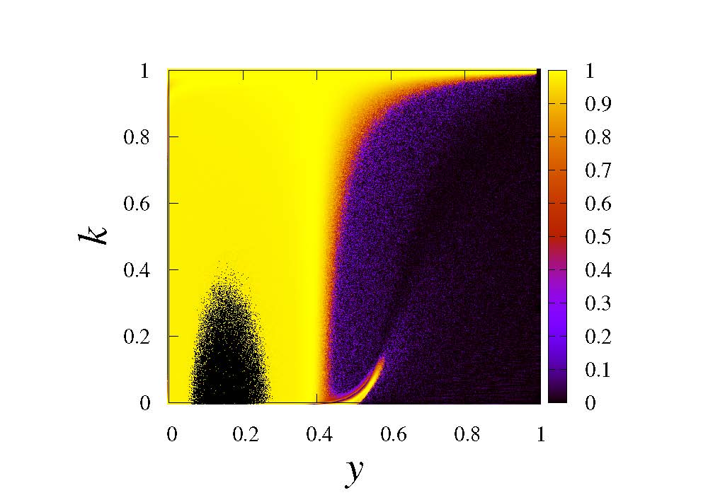
To construct this figure, we needed to perform $10^{6}$ independent simulations. Each simulation was carried out on square lattices of linear size $L=80$ with periodic boundary conditions and returned the value of $r$ obtained for a given set of the control parameters, $y$ and $k$. Here, we considered the system starting with a lattice fully ocuppied by $CO$ molecules, which means $\rho_{0}=0$ since we are using the density of empty sites as the order parameter of the model. Each value of $r$ is an average taken over 1000 samples in their first 300 MC steps without taking into account the first $N_{\min}=100$ MCsteps. As stated above, $r$ ranges from zero (black points) which means that the considered point ($y,k$) is not critical, to one (yellow points) which means that this point follows a power law and therefore is a candidate to critical point. This figure shows a large extension of yellow points, mainly before the critical point of the original ZGB model, $y\simeq 0.39$ (here named as region 1). As can be seen, there is also a small region near the discontinuous point, around $0.45\lesssim y\lesssim 0.6$ and small values of $k$, which has a set of yellow points and looks like a tail (the region 2). These behaviors can be easily explained: as the second order phase transition of the original model takes place at the point which separates the $O$ poisoned phase from the beginning of the reactive state where the production of $CO_{2}$ molecules starts, any value of $k$ does not influence this transition substantially. However, for the discontinuous phase transition this argument does not hold since at this point, even a small value of $k$ can avoid the poisoning of the surface with $CO$ molecules and, therefore, $k$ substantially influences the transition to the point of eliminating the discontinuous phase transition.

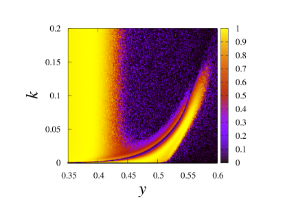
In Fig. 2, we highlight the region that presents an extension coming from the continuous phase transition ($y\approx 0.39$ and $k=0$) and that lasts up to $y\approx 0.58$ and $k\approx 0.15$ which is close to discontinuous phase transition of the original model $y\approx 0.53$ and $k=0$.  

Figure 2: A highlight of the coefficient of determination $r$ as function of $y$ and $k$ for the ZGB model with desorption of $CO$ molecules. We can observe an extension that ends after the discontinuous phase thansition point ($y\approx 0.53$) of the model without desorption ($k=0$). This extension comes from continuous phase transition of the original ZGB model ($y\approx 0.39$ and $k=0$).

Before analysing these two regions in detail, it is important to improve Fig. 1 in order to find points with best coefficients of determination. Figure 3 shows the refinement of Fig. 1 for higher values of $r$: $r\geq 0.98$, 0.99, 0.999, and 0.9995.

Figure 3: Refinement process of the coefficient of determination for (a) $r\geq 0.98$, (b) $r\geq 0.99$, (c) $r\geq 0.999$, and (d) $r\geq 0.9995$.

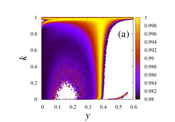
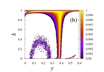
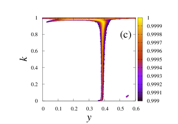
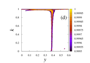
This figure shows a narrowing of the yellow points in both regions when one considers only $r\geq 0.98$ to $r\geq 0.9995$. Figure 3 (b) shows that, for $r\geq 0.99$, the region 1 splits into two parts: the first one looks like an upside-down bow and the second one is a straight vertical line which starts at $y\simeq 0.39$ and $k=0$ and increases to around $k=1$ when two branches arise in both sides of the diagram. On the other hand, the region 2 presents two well defined lines which meet each other in $y\sim 0.56$ and $k\sim 0.07$. A similar analysis can be done for $r\geq 0.999$ (see Fig. 3 (c)) with only a decrease of yellow points. So, as $r\geq 0.999$ is a good value for the coefficient of determination, all these points can be considered as candidates to phase transition points. However, as we are looking for higher values of $r$, we consider in our study only values of $r\simeq 0.9995$ as presented in Fig. 3 (d). This figure shows that the region 1, around the critical adsorption rate of the original model ($y\simeq 0.39$) and for all values of $k$, is not affected by the desorption of $CO$ molecules albano1992 ; chan2015 . However, the discontinuous phase transition of the original ZGB model ($y\simeq 0.53$) and $k\simeq 0$ disappears even for very small values of $k$ tome1993 ; chan2015 . In this case, only few points appear in region 2.

In order to analyse these points, and more precisely the characteristics of their proximities, we consider the region $0.44\leq y\leq 0.56$ and $0\leq k\leq 0.09$ with the refinement $r\geq 0.98$, as shown in Fig. 4.

Figure 4: Figure (a) shows a small part of the region 2 ($0.44\lesssim y\lesssim 0.56$ and $k\lesssim 0.09$) corresponding to the two curves that, after the refinement, lead to a single point. The vertical dashed lines correspond to different values of $y$: (i) $y=0.530$, (ii) $y=0.536$, (iii) $y=0.542$, and (iv) $y=0.552,$ where the coefficient of determination $r$ is calculated as function of $k$. Figure (b) shows $r\times k$ for these values of $y$. We can observe that the double peaks observed in the plots (i), (ii), and (iii) culminates in an single peak shown in the plot (iv). The inset in the plot (d) is a zoom in order to verify the existence of a unique peak.

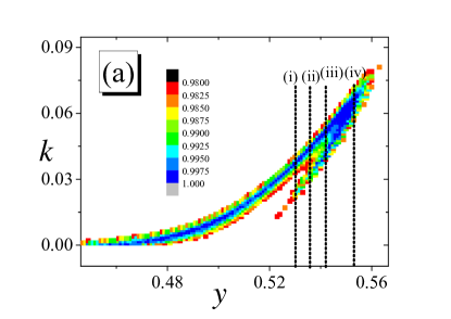
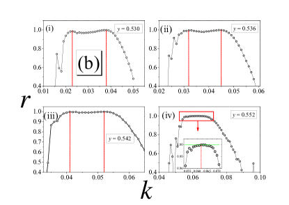
As can be seen, this figure highlights the two curves presented in Fig. 3 (a) which lie at a give point. In order to characterize the phenomena related to this region we choose four values of $y$: 0.530, 0.536, 0.542, and 0.552, and calculate the coefficient of determination $r$ for $0\leq k\leq 0.09$ with $\Delta k=0.001$. The vertical dashed lines presented in Fig. 4 (a) indicate where our analysis is performed. We can observe that three of these vertical lines cross both curves which means a double peak in a plot of $r\times k$ as shown in Fig. 4 (b) for: (i) $y=0.530$, (ii) $y=0.536$, and (iii) $y=0.542$. However, the vertical line for $y=0.552$ [Fig. 4 (a)] crosses the curve only once, i.e., there is only a single peak in Fig. 4 (b): (iv). The inset plot in this figure corresponds only to a zoom which indeed verifies the existence of a unique peak. As found in previous works albano2001b ; fernandes2016 , the two peaks are related to pseudo critical points (here interpreted from a nonequilibrium simulations’ point of view) which characterize the discontinous phase transitions (weak first order phase transitions). Here, it is worth to mention that in a previous work, Tomé and Dickman tome1993 found, for $y=0.54212$ and $k=0.0406$, an critical adsorption rate associated with an Ising-like point. However, in our study, we believe that this point must be related to a single peak, as shown in the last plot of Fig. 4 (b). According to our simulations the best candidate to this Ising-like point is slightly after $y=0.552$ and $k=0.064$. In fact, our best value of the coefficient of determination, $r=0.99984$ was obtained for $y=0.554$ and $k=0.064$.

At this point, two important questions arise. Firstly, as shown in Ref. tome1993 , is this point an Ising-like critical point? Secondly, is the narrow extension of points that grow up from $k=0$ to $k=1$ nearby $y\approx 0.390$ critical? If so, what can we say about its universality class?

In the next subsection, we look into some points of the region 1, Fig. 3 (d), and the point corresponding to the best value of $r$ of the region 2, $y=0.554$ and $k=0.064$. The analysis is carried out by means of nonequilibrium MC simulations.

III.2 Critical exponents

In this subsection, we obtain the critical exponents $\delta=\beta/\nu_{\parallel}$ and $\theta$ for some critical points through nonequilibrium MC simulations of the ZGB model with $CO$ desorption. All results were obtained for the following set of parameters: $L=160$, $N_{MC}=300$, and 5000 samples. The results are averages obtained through 5 different time evolutions and the error bars are obtained from them. To study the region 1, we decided to consider some values of $k$, equally spaced, and look for values of $y_{\text{best}}$ which correspond to the best value of $r_{\text{best}}$. The values of $k$, $y_{\text{best}}$, and $r_{\text{best}}$ are shown in Table 1. As shown in the second row of this table, the values of $y$ are very close to the value of the critical adsorption rate of the original ZGB model, $y=0.388$.

$k$	$0.1$	$0.2$	$0.3$	$0.4$	$0.5$	$0.6$	$0.7$	$0.8$	$0.9$
$y_{\text{best}}$	$0.387$	$0.388$	$0.387$	$0.388$	$0.391$	$0.388$	$0.391$	$0.390$	$0.392$
$\delta_{\text{best}}$	$0.4838(6)$	$0.4527(4)$	$0.4797(7)$	$0.4587(6)$	$0.4065(2)$	$0.4581(4)$	$0.4146(5)$	$0.4218(2)$	$0.3953(1)$
$r_{\text{best}}$	$0.999784$	$0.999767$	$0.999801$	$0.999867$	$0.999718$	$0.999928$	$0.999915$	$0.999953$	$0.999975$
$\delta$	$0.4532(3)$	$0.4527(3)$	$0.4546(4)$	$0.4587(6)$	$0.4587(5)$	$0.4581(4)$	$0.4515(4)$	$0.4396(5)$	$0.4153(3)$
$r$	$0.999770$	$0.999767$	$0.999650$	$0.999867$	$0.999541$	$0.999928$	$0.999898$	$0.999469$	$0.999829$
$\theta$	$0.24(1)$	$0.23(2)$	$0.23(2)$	$0.23(1)$	$0.22(1)$	$0.21(2)$	$0.21(1)$	$0.21(1)$	$0.21(1)$

Table 1: Critical exponents estimated for the refined points of the region 1

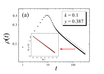
In order to obtain the critical exponents, we first consider the simulations starting with the initial condition $\rho_{0}=0$, i.e., where all sites of the lattice are initially occupied by $CO$ molecules, and we also expect a power law described by Eq. (8). Figure 5 (a) ilustratres the time evolution of $\rho(t)$ in $\log\times\log$ scale for one particular case: $k=0.1$ and $y=0.387$. We can observe that after an initial transient, $\rho(t)$ decays (the inset plot shows the corresponding linear fit in $\log\times\log$ scale). The error bars taken over 5 different diferent seeds are indeed very small. The values obtained for $\delta\ (\delta_{\text{best}})$ corresponding to the best $y=y_{\text{best}}$ are shown in the third row of Table 1. The values are close to $\delta=0.451$ voigt1997 . However, the results present a certain variation and do not permit us to assert that the points found in region 1 belong to the DP universality class. The values of coefficient of determination for these points are presented in the fourth row of Table 1.

Since the values of $y$ (second row) are very close to $y=0.388$ (in fact, this value appears in four of the nine values presented in Table 1) we also carried out simulations by considering the same values of $k$ but kept $y=0.388$. The coefficient of determination is still very close to 1, as shown in the sixth row of Table 1, and the results for the exponent $\delta$ are surprisingly. Now we have $\delta$ even more closer to the value of the DP universality class (see the row 5 of the table).

Figure 5: Plot (a) shows the time evolution of $\rho(t)$ in $\log\times\log$ scale for one particular case: $y=0.387$ and $k=0.1$ when all sites are inittialy filled with $CO$ molecules. We can observe that after a transient, the system decays according to the power law given by Eq. (7) (the inset plot highlights the robustness of this power law). Plot (b) shows the initial growing of $\rho(t)$ when the initial lattice is fully ocuppied by $O$ atoms except for a vacant site located at the center of the lattice. We show the power laws for $k=0.1$, $0.2$, …, $0.9$ and $y=0.388$.

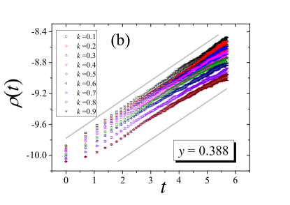
Thus, our results suggest that the points for the region 1 are critical ones and may belong to the DP universality class, but further studies must be performed in order to confirm (or not) this assertion. However, we have two more results to present in this work and which reinforces our previous estimates. First, we show the results related to the exponent $\theta$. Here, it is important to note that the initial transient where $\rho(t)$ increases before decaying as $\rho(t)\sim t^{-\delta}$, does not correspond to the critical initial slip where the exponent $\theta$ is usually obtained. In fact, this exponent is not expected for that initial condition. In addition, this initial transient lasts only for few steps (less than 10 MC steps). So we performed simulations for those same points presented in Table 1 with the initial condition where all sites are ocuppied by $O$ atoms but a single site that remains vacant at the center of the lattice, i.e., $\rho_{0}=1/L^{2}$. The time evolution of $\rho(t)$ (given by Eq. (8)) is shown in Fig.5 (b). The gray lines introducted in this figure work as directions to observe that power laws are approximately parallel lines in $\log\times\log$ scale. The seventh row of Table 1 presents the exponents $\theta$ for all considered points. These values are very close to $\theta=0.230$ found for the two-dimensional DP model voigt1997 . The error bars are bigger for this initial condition as can also be observed in Fig. 5 (b) generating uncertainties in the second decimal digit.

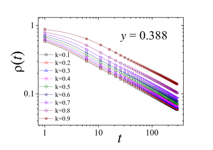
Secondly, it is also possible to study the behavior of $\rho(t)\sim t^{-\delta}$ when all initial sites are vacant, since we expect this behavior specifically for this initial condition when considering the density of vacant site as the order parameter of the model. We verifed that, in this case, the exponent $\delta$ corresponds exactly to what is expected when $\rho_{0}=1$, giving $\delta\approx 0.45$ for all values of $k$ as can be observed in Fig. 6 which present curves with aproximately the same slope (parallel lines).

Figure 6: Time evolution of $\rho(t)$ for $y=0.388$ when we start with all sites vacant ($\rho_{0}=1$) for $k=0.1$, $0.2$, …, $0.9$.

Since we unveiled the region 1, let us briefly explore the region 2 which, according to the previous subsection, culminates in a point corresponding to a unique peak for the coefficient of determination, after a succession of double peaks (pseudo critical points). For this point ($y=0.554$ and $k=0.064$), we consider the initial lattice being fully occupied with $CO$ molecules. Figure 7 shows the critical initial slip for the density of vacant sites as function of $t$, in $\log\times\log$ scale.

Figure 7: Time evolution of density of vacant sites, $\rho(t)\times t$, for $y=0.554$ and $k=0.064$ when we start the simulation with all sites ocuppied by $CO$ molecules. The initial slip corresponds to the exponent $\theta$.

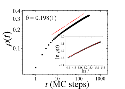
The slope of this curve gives

$$\theta=0.198(1)$$ (10)

and is in fair agreement with the results found for the Ising model, $\theta\approx 0.193$ zheng1998 . Our estimate identifies this critical point as belonging to the Ising universality class, exactly as predicted in Ref.tome1993 for the static exponent $\nu$ for a point slithly before ours, $y=0.54212$ and $k=0.0406$.

In this work, we did not perform a complete study of the critical exponents of this point since this was not our main purpose and, in addition, the topic deserves a better compreension about the exact relationship between magnetic models and absorbing state models. We also verified that the choise of both order parameter and the initial condition seems to be very important to estimate the critical exponents. So, these topics will be addressed in a further work.

IV Conclusions

In this paper, we studied the ZGB model with desorption of $CO$ molecules through nonequilibrium Monte Carlo simulations and showed for the first time that it can belong to the DP and Ising universality classes, depending on the values of the $CO$ adsorption rate, $y$, and of the $CO$ desorption rate, $k$. We presented the diagram $k\times y$ obtained through the optimization of the coefficient of determination and showed that the region belonging to the DP universality class is composed by a line of critical points extending from $0\leq k\leq 1$ and $y\simeq 0.388$. The other region possesses two pseudo critical lines that probably intercept each other at the Ising-like critical point, $y=0.554$ and $k=0.064$.

References

- (1) T. Tome and R. Dickman, Phys. Rev. E 47, 948 (1993).
- (2) H.K. Janssen, B. Schaub, and B. Schmittmann, Z. Phys. B: Condens. Matter 73, 539 (1989).
- (3) D.A. Huse, Phys. Rev. B 40, 304 (1989).
- (4) B. Zheng, Int. J. Mod. Phys. B, 12, 1419 (1998).
- (5) B. Zheng and H.J. Luo, Phys. Rev. E 63, 066130 (2001).
- (6) E.V. Albano and M.A. Muñoz, Phys. Rev. E 63, 031104 (2001).
- (7) R. da Silva, N.A. Alves, and J.R. Drugowich de Felício, Phys. Lett. A 298, 325 (2002).
- (8) R. da Silva, N.A. Alves, and J.R. Drugowich de Felício, Phys. Rev. E 66, 026130 (2002).
- (9) E. Arashiro and J.R. Drugowich de Felício, Phys. Rev. E 67, 046123 (2003).
- (10) R. da Silva and J.R. Drugowich de Felício, Phys. Lett. A 333, 277 (2004).
- (11) B.C.S. Grandi and W. Figueiredo, Phys. Rev. E 70, 056109 (2004).
- (12) H.A. Fernandes, J.R. Drugowich de Felício, and A.A. Caparica, Phys. Rev. B 72, 054434 (2005).
- (13) , I.A. Hadjiagapiou, A. Malakis, and S.S. Martinos, Physica A 356, 563 (2005).
- (14) H.A. Fernandes and J.R. Drugowich de Felício, Phys. Rev. E 73, 057101 (2006).
- (15) H.A. Fernandes, E. Arashiro, J.R. Drugowich de Felício, and A.A. Caparica, Physica A 366, 255 (2006).
- (16) H.A. Fernandes, Roberto da Silva, and J.R. Drugowich de Felício, J. Stat. Mech. (2006) P10002.
- (17) V.V. Prudnikov, P.V. Prudnikov, A.S. Krinitsyn, A.N. Vakilov, E.A. Pospelov, and M.V. Rychkov, Phys. Rev. E 81, 011130 (2010).
- (18) R. da Silva, H.A. Fernandes, J.R. Drugowich de Felício, and W. Figueiredo, Comp. Phys. Comm. 184, 2371 (2013).
- (19) R. da Silva, N. Alves, Jr., and J.R. Drugowich de Felício, Phys. Rev. E 87, 012131 (2013).
- (20) R. da Silva, H.A. Fernandes, and J.R. Drugowich de Felício, Phys. Rev. E 90, 042101 (2014).
- (21) A. Chiocchetta, A. Gambassi, S. Diehl, and J. Marino, Phys. Rev. B 94, 174301 (2016).
- (22) H.A. Fernandes, R. da Silva, A. A. Caparica, J. R. Drugowich de Felicio, Phys. Rev. E 95, 042105 (2017)
- (23) R. da Silva, J.R. Drugowich de Felício, and A.S. Martinez, Phys. Rev. E 85, 066707 (2012).
- (24) E. Arashiro, J.R. Drugowich de Felício, and U.H.E. Hansmann, Phys. Rev. E 73, 040902 (2006); J. Chem. Phys. 126, 045107 (2007).
- (25) M.-B. Luo and C.-J. Qian, Polymer, 47, 1451 (2006).
- (26) R. da Silva, R. Dickman, and J.R. Drugowich de Felício, Phys. Rev. E 70, 067701 (2004).
- (27) R. da Silva, H.A. Fernandes, J. Stat. Mech. (2015) P06011.
- (28) U. Basu, V. Volpati, S. Caracciolo, and A. Gambassi, Phys. Rev. Lett. 118, 050602 (2017).
- (29) E.S. Loscar, C.G. Ferrara, and T.S. Grigera, J. Chem. Phys. 144, 134501 (2016).
- (30) E.S. Loscar, D.A. Martin, and T.S. Grigera, J. Chem. Phys. 147, 21 (2017).
- (31) E.V. Albano, Phys. Lett. A 288, 73 (2001).
- (32) H.A. Fernandes, R. da Silva, E.D. Santos, P.F. Gomes, and E. Arashiro, Phys. Rev. E 94, 022129 (2016).
- (33) E.V. Albano, M.A. Bab, G. Baglietto, R.A. Borzi, T.S. Grigera, E.S. Loscar, D.E. Rodriguez, M.L.R. Puzzo, and G.P. Saracco, Rep. Prog. Phys. 74, 026501 (2011).
- (34) J.W. Evans, Langmuir 7, 2514 (1991).
- (35) E.V. Albano, Surf. Sci. 306, 240 (1994).
- (36) M.F. de Andrade and W. Figueiredo, Phys. Rev. E 81, 021114 (2010).
- (37) M.F. de Andrade and W. Figueiredo, J. Chem. Phys. 136, 164502 (2012).
- (38) M. Ehsasi, M. Matlock, O. Frank, J.H. Block, K. Christmann, F.S. Rys, and W. Hirschwald, J. Chem. Phys. 91 4949 (1989).
- (39) K. Christmann, Introduction to Surface Physical Chemistry (Steinkopff Verlag, Darmstadt, 1991), pp. 1274.
- (40) R. Imbhil and G. Ertl, Chem. Rev. 95, 697 (1995).
- (41) R.M. Ziff, E. Gulari, and Y. Barshad, Phys. Rev. Lett. 56, 2553 (1986).
- (42) C.A. Voigt, R.M. Ziff, Phys. Rev. E 56 R6241 (1997).
- (43) R.M. Ziff and B.J. Brosilow, Phys. Rev. A, 46 4630 (1992).
- (44) P. Meakin and D.J. Scalapino, J. Chem. Phys. 87, 731 (1987).
- (45) R. Dickman, Phys. Rev. A 34, 4246 (1986).
- (46) J. Marro and R. Dickman, Nonequilibrium Phase Transitions in Lattice Models (Cambridge University Press, Cambridge, U.K., 1999).
- (47) P. Fischer and U.M. Titulaer, Surf. Sci. 221, 409 (1989).
- (48) M. Dumont, P. Dufour, B. Sente, and R. Dagonnier, J. Catal. 122, 95 (1990).
- (49) A.V. Albano, Appl. Phys. A: Mater. Sci. Proc. 55, 226 (1992).
- (50) B.J. Brosilow and R.M. Ziff, Phys. Rev. A 46 , 4534 (1992).
- (51) T. Matsushima, H. Hashimoto, and I. Toyoshima, J. Catal. 58, 303 (1979).
- (52) G. M. Buendía and P.A. Rikvold, Phys. Rev. E 88, 012132 (2013).
- (53) C.H. Chan and P.A. Rikvold, Phys. Rev. E 91, 012103 (2015).
- (54) I. Jensen and H. Fogedby, Phys. Rev. A 42, 1969 (1990).
- (55) H.P. Kaukonen and R.M. Nienimen, J. Chem. Phys. 91, 4380 (1989).
- (56) G.M. Buendía, P.A. Rikvold, Phys. A. 424, 217 (2015).
- (57) B.C.S. Grandi and W. Figueiredo, Phys. Rev. E 65, 036135 (2002).
- (58) G.L. Hoenicke and W. Figueiredo, Phys. Rev. E 62, 6216 (2000).
- (59) G. M. Buendía and P.A. Rikvold, Phys. Rev. E 85, 031143 (2012).
- (60) G.L. Hoenicke, M.F. de Andrade, and W. Figueiredo, J. Chem. Phys. 141, 074709 (2014).
- (61) J. Satulovsky and E.V. Albano, J. Chem. Phys. 97, 9440 (1992).
- (62) E.V. Albano, Surf. Sci. 235, 351 (1990).
- (63) B.J. Brosilow, E. Gulari, and R.M. Ziff, J. Chem. Phys. 98, 674 (1993).
- (64) K. S. Trivedi, Probability and Statistics with Realiability, Queuing, and Computer Science and Applications, 2nd ed. (John Wiley and Sons, Chichester, 2002).
- (65) W. Evans and M. S. Miesch, Phys. Rev. Lett. 66, 833 (1991).
- (66) H. Hinrichsen, Adv. Phys. 49, 815 (2000).