Path-Following through Control Funnel Functions

Abstract

We present an approach to path following using so-called control funnel functions. Synthesizing controllers to “robustly” follow a reference trajectory is a fundamental problem for autonomous vehicles. Robustness, in this context, requires our controllers to handle a specified amount of deviation from the desired trajectory. Our approach considers a timing law that describes how fast to move along a given reference trajectory and a control feedback law for reducing deviations from the reference. We synthesize both feedback laws using “control funnel functions” that jointly encode the control law as well as its correctness argument over a mathematical model of the vehicle dynamics. We adapt a previously described demonstration-based learning algorithm to synthesize a control funnel function as well as the associated feedback law. We implement this law on top of a 1/8th scale autonomous vehicle called the Parkour car. We compare the performance of our path following approach against a trajectory tracking approach by specifying trajectories of varying lengths and curvatures. Our experiments demonstrate the improved robustness obtained from the use of control funnel functions.

I INTRODUCTION

Recent advances in motion planning have brought truly autonomous systems closer to becoming a reality. However, one of the main challenges is their safety. Plan execution may fail because of considerable uncertainties such as disturbances, imprecise measurements, and modeling. Such failures can lead to safety violation with catastrophic consequences. Given a reference trajectory with associated timing, a straightforward solution is to design a feedback control which tracks the reference trajectory and reduces tracking errors. Another idea is to use “path-following” where the goal is to track a path without timing constraints. Path-following techniques provide smooth convergence to the reference trajectory while avoiding input saturation [1, 2], and are more robust with respect to measurement errors and external disturbances [3]. In this paper, we investigate path-following techniques to improve robustness and safety for plan execution through control funnel functions.

Figure 1: Safe tracking with control funnels: the black box depicts an obstacle, solid red line shows the reference trajectory generated by the planner. The projection of the funnel on $x$-$y$ plane is shown in green. The green circle at the right is the head of the funnel and the one to the left is the tail. The blue region enlarges the funnel to account for the non-zero size of the vehicle.

First, we reformulate the problem as a path following problem that adds an extra control input to the system to decide how fast to move along the reference trajectory. This naturally allows our approach to speed up/slow down progress along the reference trajectory. Furthermore, our method is based on control funnel functions inspired by the concepts of control funnels [4, 5] and control barrier functions [6]. Given a reference trajectory segment and a desired “safe region” around the trajectory, a control funnel function guarantees that the system moves along one end of the trajectory to another while remaining inside the safe region. We use a previously-developed framework to synthesize control funnels automatically given the vehicle dynamics, the reference trajectory, and the surrounding safe region [7].

We have implemented our method using a standard single-track model for capturing the ground vehicle dynamics. The resulting controllers are then tested on a $\frac{1}{8}^{th}$ scale vehicle platform called the Parkour car developed at CU-Boulder. Using our approach, we successfully synthesize controllers for numerous reference trajectories and demonstrate the ability of the controller synthesized on a toy model to drive an actual vehicle in the lab. We also show that, when contrasted with trajectory tracking, path following approaches provide a higher level of robustness as shown by some of our experiments that involved large disturbances applied to the car during motion.

In the rest of this section we review the literature. We discuss previously developed methods and our notations in Section II. Sections III and IV present our contributions. Finally, in Section V, we discuss our experimental results.

I-A Related Work

Stability for autonomous vehicles is a challenging problem. Brockett [8] showed that even a simple unicycle model cannot be stabilized using continuous feedback laws. However, continuous feedback laws exist for stabilization to non-stationary trajectories; these feedback laws are usually obtained through linearization [9]. While trajectory tracking has been widely used to solve plan execution, it has several shortcomings which are addressed using path-following. In pioneering work  [10, 11, 12, 13, 14] the velocity of the vehicle tracked a desired reference velocity and the controller is designed to steer the vehicle to the path. These path-following methods have been shown to yield a smoother convergence to the trajectory while avoiding input saturation. Beside these works, a wide diversity of approaches are used to study the path-following problem. One line of work is based on designing vector fields surrounding the path to guarantee reaching and following the path [15, 16]. Another approach is to use model predictive control [17, 18]. In this article, we consider a line of effort distinct from these others.

Hauser et al. [1] proposed the conversion of the trajectory tracking strategy to the so-called maneuver regulation strategy. The main idea is to decrease the distance between the state and the reference trajectory, not a specific point on the trajectory. The reference trajectory $\mathbf{x}_{r}(\cdot)$ is parameterized using a variable $\theta$ (instead of time) and distance is defined as a function of $\mathbf{x}-\mathbf{x}_{r}(\theta)$. $\theta$ and treated as a variable. An update law (timing law) is then applied to ensure proper change of $\theta$. Hauser and Hindman showed that this maneuver regulation trick would yield a system that avoids input saturation. Similarly, Pappas [2] showed that by re-parameterizing the trajectory, one could avoid input saturation. Subsequently, Encarnacao et al. [19] extended the technique for the output maneuvering problem on a restricted set of dynamics. m

Following Hauser et al. [1], others have divided the task into two parts. The first task is to reach and follow the reference trajectory using the variable $\theta$ (instead of time), and the second task is to improve the solution using an extra control input $\theta$. For example, in Skjetne et al. [20], first the system output is stabilized, and then a control law for $\theta$ is used to adjust the velocity. In this work, we use the extra freedom to control $\theta$ for increasing robustness. More specifically, this extra degree of freedom allows us to design more robust control Lyapunov functions (CLFs) from which we extract the feedback as well as the timing law.

Control Lyapunov functions were originally introduced by Sontag [21, 22]. Synthesis of CLFs is hard, involving bilinear matrix inequalities (BMIs) [23, 5]. Standard approaches such as alternating minimization result often do not converge to a solution. To combat this, Majumdar et al. use LQR controllers and their associated Lyapunov functions for the linearization of the dynamics as good initial seed solutions [5]. In contrast, recent work by some of the authors remove the bilinearity by using a demonstrator in the form of a MPC controller [7]. Furthermore, this approach avoids local saddle points and has a fast convergence guarantee.

Aguiar et al. [24] argue that there are performance limitations for systems with unstable zero dynamics if one uses trajectory tracking. However, using an extra control input $\theta$, this restriction vanishes. The timing law in this work is designed as a function of $\theta$ and its higher derivatives.

Egerstedt et al. [3] develop a method where the reference point dynamics are governed by tracking error feedback. Similarly, Faulwasser et al. [25] proposed designing the timing law as a function of $\theta$, tracking error, and their higher derivatives. For example, one can design a timing law which slows down the progress of $\theta$ when the distance between the state and the reference is large. They also combine the idea of path-following with control funnels. They Similarly, we use control funnels to provide formal guarantees. However, the funnel is constructed using a CLF. Besides this, the timing law in our work is a function of the state $\mathbf{x}$ and depends on the structure of the CLF.

II BACKGROUND

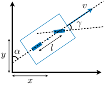
This paper investigates CLF-based path following focusing on applications to ground vehicles. We will use the well-known bicycle model, whose state consists of its position ($x$ and $y$), its orientation ($\alpha$), and velocity ($v$) [26, 3]. The rear axle is perpendicular to the bicycle’s axis, the front wheel’s orientation can be adjusted to steer the vehicle (see Figure 2). Let $\gamma$ be the angle between the front axle and the bicycle axis (Fig. 2). We will assume that $\gamma\in[-\frac{\pi}{4},\frac{\pi}{4}]$ is a control input to the model. Also, the thrust applied to the vehicle is $\mathcal{T}\in[-4,4]$. The model has the following dynamics:

$$\begin{array}[]{l}\accentset{\mbox{\large.}}{x}\ =\ v\sin(-\alpha),\ \ \accentset{\mbox{\large.}}{y}\ =\ v\cos(\alpha)\\ \accentset{\mbox{\large.}}{\alpha}\ =\ \frac{v}{l}\tan({\color[rgb]{0,0,1}\definecolor[named]{pgfstrokecolor}{rgb}{0,0,1}\gamma}),\ \ \accentset{\mbox{\large.}}{v}\ =\ {\color[rgb]{0,0,1}\definecolor[named]{pgfstrokecolor}{rgb}{0,0,1}\mathcal{T}}\,,\end{array}$$ (1)

wherein $l$ is the distance between the wheels and the control inputs to the model $({\color[rgb]{0,0,1}\definecolor[named]{pgfstrokecolor}{rgb}{0,0,1}\gamma},{\color[rgb]{0,0,1}\definecolor[named]{pgfstrokecolor}{rgb}{0,0,1}\mathcal{T}})$ are shown in blue.

Figure 2: A Schematic Diagram of the Bicycle Model.

We will use this model to analyze the behavior of ground vehicles. In this paper, we will study the design of control inputs to solve the problem of controlling the vehicle to follow a given trajectory. Such trajectories are generated using planning algorithms such as RRTs and are often designed to avoid obstacles in the workspace [27].

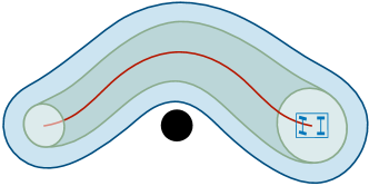
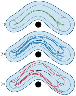
As an example, consider a scenario where the vehicle moving with speed $2\textsf{m/s}$ needs to circumnavigate an obstacle as shown in Fig. 1. First, the planner generates a reference trajectory shown with the solid red line. Note that, by design, the reference trajectory keeps some distance from the obstacle.

To guarantee safety and trajectory tracking at the same time, we use a control funnel [4] (the green region in Fig. 1) which contains the reference trajectory. The corresponding control law for a funnel guarantees that once the state is inside the funnel, it remains in the funnel until it reaches the desired target set of states. In other words, the system safety in the tracking process is formally guaranteed. In this work, we wish to improve the process of funnel design to increase robustness. Our funnel design technique is based on stability analysis which is discussed first.

II-A Stability Analysis

The dynamics for autonomous vehicles can be modeled with Euler equations to study the behavior of these systems. In a continuous time setting, the state of the system $\mathbf{x}\in\mathbb{R}^{n}$ updates w.r.t. an ordinary differential equation. Formally, $\accentset{\mbox{\large.}}{\mathbf{x}}=f(\mathbf{x},\mathbf{u})$, where $\accentset{\mbox{\large.}}{\mathbf{x}}$ is the derivative of $\mathbf{x}$ w.r.t. time and $\mathbf{u}\in\mathbb{R}^{m}$ is the control input. Stability is a fundamental property of dynamical systems. Numerous control problems can be viewed as controlling a given system to stabilize to a given equilibrium state $\mathbf{x}_{r}$ or an “equilibrium” reference trajectory $\mathbf{x}_{r}(t)$. Control Lyapunov functions (CLF) are a powerful tool for designing such stabilizing controls [22, 28]. We first describe CLFs for stabilizing to an equilibrium state.

Definition 1 (Control Lyapunov Functions)

A CLF $V$ is a smooth and radially unbounded function that maps each state to a real non-negative value, such that (a) $V(\mathbf{x}_{r})=0$ and $V(\mathbf{x})>0$ for all $\mathbf{x}\not=\mathbf{x}_{r}$, and (b) $(\forall\ \mathbf{x}\not=\mathbf{x}_{r})\ (\exists\mathbf{u})\ \accentset{\mbox{\large.}}{V}(\mathbf{x},\mathbf{u})<0$, wherein $\accentset{\mbox{\large.}}{V}$ is the Lie-derivative of $V$ w.r.t. $f$: $\accentset{\mbox{\large.}}{V}(\mathbf{x},\mathbf{u})=\nabla V\cdot f(\mathbf{x},\mathbf{u})$.

Condition (a) ensures that the value of $V$ is zero at the equilibrium and strictly positive everywhere else. Condition (b) ensures that for any state, we can find a control input that can achieve an instantaneous decrease to the value of $V$. In this sense, CLFs are equivalent to artificial potential functions over the state space [29]. Having a CLF, one can design a feedback law which always decreases the value of $V$ and therefore stabilizes the system to the equilibrium point. For instance, Sontag provides a simple means to extract a feedback law from a given CLF [21].

II-B Trajectory Tracking vs. Path Following

Another form of stability appears in trajectory tracking, wherein the goal is to stabilize to a reference trajectory $\mathbf{x}_{r}(t)$. Formally, let $\mathbf{x}_{d}(t):\ \mathbf{x}(t)-\mathbf{x}_{r}(t)$ describe the “deviation” from the reference trajectory state at time $t$. The goal is to stabilize $\mathbf{x}_{d}$ to the equilibrium $\mathbf{0}$ under the time-varying reference frame that places $\mathbf{x}_{r}(t)$ as the origin at time $t$. The dynamics for $\mathbf{x}_{d}$ is defined as: $\accentset{\mbox{\large.}}{\mathbf{x}}_{d}=f(\mathbf{x},\mathbf{u})-\mathbf{r}(t)$, wherein $\accentset{\mbox{\large.}}{\mathbf{x}}_{r}=\frac{d\mathbf{x}_{r}}{dt}=\mathbf{r}(t)$.

One of the key drawbacks of trajectory tracking is that it specifies the reference trajectory $\mathbf{x}_{r}(t)$ along with the reference timing, wherein the state $\mathbf{x}_{r}(t)$ must ideally be achieved at time $t$. This poses a challenge for control design unless the timing is designed very carefully. Imagine, a reference trajectory that traverses a winding hilly road at constant speeds. This compels the control to constantly accelerate the vehicle on upslopes only to “slam the brakes” on downhill sections [30].

Path following, on the other hand, separates these concerns by allowing the user to specify a reference (feasible) path parameterized with a scalar, $\theta$ (instead of time), $\mathbf{x}_{r}(\theta)$ yields a state for each $\theta$ and $\frac{d\mathbf{x}_{r}}{d\theta}=\mathbf{r}(\theta)$. As proposed by Hauser et al., one could define $\Pi$ as a function that maps a state $\mathbf{x}$ to the closest state on the reference trajectory $\mathbf{x}_{r}(\cdot)$, using an auxiliary map $\pi$  [1, 31]:

$$\pi(\mathbf{x}):\ \underset{\theta}{\mbox{argmin}}\ ||\mathbf{x}-\mathbf{x}_{r}(\theta)||_{P}^{2}\ \,,\ \Pi(\mathbf{x}):\mathbf{x}_{r}(\pi(\mathbf{x}))$$

where $||\mathbf{x}||_{P}^{2}:\ \mathbf{x}^{t}P\mathbf{x}$ is a Lyapunov function for the linearized dynamics around the reference trajectory. In order to stabilize the system to the reference path, Hauser et al. propose to decrease the value of $||\mathbf{x}-\Pi(\mathbf{x})||_{P}^{2}$. However, as the projection function $\pi$ can get complicated, they use local approximations of $\pi$.

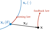
Following this, others have proposed to design a control law for a virtual input $u_{0}$ that controls $\theta$ as a function of time (called the timing feedback law), or in other words, the progress (or sometimes regress) along the reference [20, 24]. Therefore, the deviation is now defined as $\mathbf{x}_{d}(t):\ \mathbf{x}(t)-\mathbf{x}_{r}(\theta(t))$ wherein $\frac{d\theta}{dt}=u_{0}$. As depicted in Fig. 3, $\theta$ is mapped to a state on the path $\mathbf{x}_{r}(\theta)$. For example Faulwasser et al. [25] design the timing law as a function of $\theta$, the deviation ($\mathbf{x}_{d}$ for state feedback systems), and their higher derivatives:

$$g(\theta^{(k)},\mathbf{x}_{d}^{(k)},\ldots,\theta,\mathbf{x}_{d},u_{0})=0\,,$$

wherein $\theta^{(k)}$ is the $k^{th}$ derivative of $\theta$. However, defining the function $g$ is a nontrivial problem.

Figure 3: Schematic View of a System along the Parameterized Path.

III PATH-FOLLOWING USING CLF

We now present the design of a path following scheme by specifying a timing law as well as control for deviation from the reference trajectory based on a control Lyapunov function. Let us define a new coordinate system, in which the state of the system is $\mathbf{z}^{t}:[\theta,\mathbf{x}_{d}^{t}]$, wherein $\mathbf{x}(t)=\mathbf{x}_{d}(t)+\mathbf{x}_{r}(\theta(t))$ is the original state of the system. Also, the control inputs are $\mathbf{v}^{t}:[u_{0},\mathbf{u}^{t}]$. We assume $\theta$ is directly controllable using $u_{0}$: $\accentset{\mbox{\large.}}{\theta}=u_{0}$. Therefore, $\accentset{\mbox{\large.}}{\mathbf{x}}_{r}=\frac{d\mathbf{x}_{r}}{d\theta}\accentset{\mbox{\large.}}{\theta}=\mathbf{r}(\theta)u_{0}$. and thus

$$\accentset{\mbox{\large.}}{\mathbf{x}}_{d}=f(\mathbf{x}_{d}+\mathbf{x}_{r}(\theta),\mathbf{u})-\mathbf{r}(\theta)u_{0}\,.$$

First, our goal is to design a control that seeks to stabilize $\mathbf{x}_{d}=0$. We define a CLF as a function $V$ over $\mathbf{x}_{d}$, but independent of $\theta$, that respects the following constraints:

$$\begin{array}[]{l}\noindent\textbf{(A)}:\ V(\mathbf{0})=0\ \mbox{and}\ (\forall\mathbf{x}_{d}\neq\mathbf{0})\;V(\mathbf{x}_{d})>0\\ \noindent\textbf{(B)}:\ (\forall\ \theta,\ \mathbf{x}_{d}\neq\mathbf{0})\;(\exists\mathbf{u},u_{0})\;\accentset{\mbox{\large.}}{V}(\theta,\mathbf{x},u_{0},\mathbf{u})<0\,.\\ \end{array}$$ (2)

Note that although $V$ is a function of $\mathbf{x}_{d}$, its derivative is a function of $\mathbf{x}_{d},\theta,u_{0},\mathbf{u}$:

$$\accentset{\mbox{\large.}}{V}(\theta,\mathbf{x}_{d},u_{0},\mathbf{u}) =\nabla V(\mathbf{x}_{d})\cdot\accentset{\mbox{\large.}}{\mathbf{x}}_{d}$$

$$=\nabla V(\mathbf{x}_{d})\cdot(f(\mathbf{x}_{d}+\mathbf{x}_{r}(\theta),\mathbf{u})-\mathbf{r}(\theta)u_{0}).$$

Conditions (A) and (B) are identical to those in Definition 1, requiring the function $V$ to be positive definite, and the ability to choose controls to decrease $V$. Furthermore, note that the $(\forall\ \theta)$ quantifier in (B) guarantees that this decrease is achieved no matter where the current reference state $\mathbf{x}(\theta)$ lies relative to the current state $\mathbf{x}_{d}$. Also, we note that the value of $u_{0}$ (rate of change for $\theta$) is obtained through the feedback law derived from the CLF $V$.

Theorem 1

If there exists a function $V$ which respects Eq. (2), there exist a feedback law and a timing law (Sontag formula [21]) that are smooth almost everywhere, and stabilize to the reference trajectory.

Proof:

We appeal directly to Sontag’s result to obtain an almost-everywhere smooth feedback $\mathbf{u}(\mathbf{x}_{d},\theta)$ and $u_{0}(\mathbf{x}_{d},\theta)$ that guarantees that $\accentset{\mbox{\large.}}{V}<0$ for all $(\mathbf{x}_{d},\theta)$ with $\mathbf{x}_{d}\not=0$ [21].

Since $\accentset{\mbox{\large.}}{V}\leq 0$, and $V$ is radially unbounded, La Salle’s theorem guarantees that the dynamical system will stabilize to the 0 level set $V^{=0}:\ \{(\mathbf{x}_{d},\theta)|\ V(\mathbf{x}_{d})=0\}=\{(0,\theta)\ |\ \theta\in\mathbb{R}\}$. Note however that $V^{=0}$ is a subset of the reference trajectory since $\mathbf{x}_{d}=0$. ∎

Thus far, we have only demonstrated how CLFs can be used to decide on a timing law as well as a control to nullify the deviation to $\mathbf{0}$. However, this does not address a key requirement of progress: we need to ensure that $\accentset{\mbox{\large.}}{\theta}>0$ so that we make progress along the reference from one end to another. Other limitations include that saturation limits on $\mathbf{u}$ are not enforced, and that the avoidance of obstacles is not considered. Finally, the stability is required to be global in the entire state-space, which is very restricting. All of these restrictions will be removed in the next section.

IV PATH SEGMENT FOLLOWING PROBLEM

In the previous section, we discussed path following in a global sense using CLFs, but noted several limitations. We will refine our approach to address them in this section.

Finite Trajectories:

Consider a reference trajectory segment defined by $\mathbf{x}_{r}(\theta)$ for $\theta\in\Theta:[0,T]$. However, defining stability for such segments is cumbersome. Therefore, we discuss reachability in finite time along with safety (reach-while-stay).

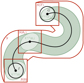
We augment the given reference trajectory by adding an initial set $\hat{I}\ni\mathbf{x}_{r}(0)$, a goal set $\hat{G}\ni\mathbf{x}_{r}(T)$, and a parameterized family of safe sets $\hat{S}(\theta)\ni\mathbf{x}_{r}(\theta)$ for $\theta\in\Theta$, such that $\hat{S}(0)\supseteq\hat{I}$ and $\hat{S}(T)\supseteq\hat{G}$. Let $\hat{S}:\ \bigcup_{\theta\in\Theta}\hat{S}(\theta)$ denote the entirety of the safe set. For convenience, we have defined $\hat{S},\hat{I},\hat{G}$ in the original state space $\mathbf{x}$. We will now define them in terms of the deviation $\mathbf{x}_{d}$ to define the following sets:

$$I :\{\mathbf{x}_{d}\ |\ \mathbf{x}_{d}+\mathbf{x}_{r}(0)\in\hat{I}\}$$

$$G :\{\mathbf{x}_{d}\ |\ \mathbf{x}_{d}+\mathbf{x}_{r}(T)\in\hat{G}\}$$

$$S(\theta) :\{\mathbf{x}_{d}\ |\ \mathbf{x}_{d}+\mathbf{x}_{r}(\theta)\in\hat{S}(\theta)\}.$$

Finally, let us denote $S:\ \bigcup_{\theta\in\Theta}S(\theta)$.

Input saturation:

Unlike infinite trajectories, here we assume initially $\theta=0$ and in the end $\theta=T$. In this setting, we must ensure progress for $\theta$ at each time-step. In other words, we wish to make sure $\accentset{\mbox{\large.}}{\theta}>0$. Recall that $\theta$ is controlled by a virtual input $u_{0}$ ($\accentset{\mbox{\large.}}{\theta}=u_{0}$). Therefore, we need input saturation for $u_{0}$ and we assume $u_{0}\in[\underline{u_{0}},\overline{u_{0}}]$, where $\underline{u_{0}}>0$ and $\overline{u_{0}}<\infty$. We also assume the reference trajectory is feasible with respect to the dynamics. To ensure that the reference trajectory remains feasible for the path following problem, we enforce that $\underline{u_{0}}\leq 1\leq\overline{u_{0}}$ as the timing law is simply $\accentset{\mbox{\large.}}{\theta}=1$ for the original reference trajectory ($\theta(t)=t$). Besides $u_{0}$, we will add saturation limits to the inputs in $\mathbf{u}$, as well. Formally we restrict $\mathbf{v}\in\mathcal{V}$ for a polytope $\mathcal{V}$.

Definition 2 (Path Segment Following Problem)

The path segment following problem, given $(S(\theta),I,G)$ and saturation constraints $\mathcal{V}$, is to derive a control feedback law $\mathbf{u}=\mathbf{u}(\theta,\mathbf{x}_{d})$ and timing law $u_{0}=u_{0}(\theta,\mathbf{x}_{d})$ such that for all initial states $\mathbf{x}_{d}(0)\in I,\theta(0)=0$, the resulting state-control trajectory of the closed loop $(\theta(t),\mathbf{x}_{d}(t),u_{0}(t),\mathbf{u}(t))$ satisfies the following conditions: (a) saturation constraints are satisfied, $(u_{0}(t),\mathbf{u}(t))\in\mathcal{V}$ for all times $t$, (b) there exists $t^{*}>0$ such that $\mathbf{x}_{d}(t^{*})\in G$, i.e, the goal is reached, and (c) for all $t\in[0,t^{*}),\ \mathbf{x}_{d}(t)\in S(\theta(t))$, while staying inside the safe set for all times until the goal is reached. Finally, note that condition (a) guarantees progress is made towards $\theta=T$ starting from $\theta=0$.

Proof Rules:

The control Lyapunov function argument can get extended to control funnels for formally satisfying the reach-while-stay property [32]. We will define a control funnel as the sublevel sets of a smooth function $V(\theta,\mathbf{x}_{d})$. For a smooth function $V$, and a relational operator $\bowtie\in\{<,\leq,=,\geq,>\}$, let us define the following families of sets that are parameterized by $\theta$: $V^{\bowtie\beta}(\theta):\{\mathbf{x}\ |\ V(\theta,\mathbf{x})\bowtie\beta\}$. Furthermore, let $V^{\bowtie\beta}:\cup_{\theta\in\Theta}\ V_{\theta}^{\bowtie\beta}$.

Definition 3 (Control Funnel Function)

A smooth function $V(\theta,\mathbf{x}_{d})$ is called a control funnel function iff the following conditions hold:

$$\begin{array}[]{lrl}\mathbf{(a)}&(\forall\mathbf{x}_{d}\in I)&V(0,\mathbf{x}_{d})<\beta\\ \mathbf{(b)}&(\forall\mathbf{x}_{d}\not\in int(G))&V(T,\mathbf{x}_{d})>\beta\\ \mathbf{(c)}&(\forall\theta\in\Theta,\mathbf{x}_{d}\not\in int(S(\theta)))&V(\theta,\mathbf{x}_{d})>\beta\\ \mathbf{(d)}&(\forall\theta\in\Theta,\mathbf{x}_{d}\in S(\theta)\cap V_{\theta}^{=\beta})&\\ &(\exists\mathbf{v}\in\mathcal{V})&\accentset{\mbox{\large.}}{V}(\theta,\mathbf{x}_{d},\mathbf{v})<0.\end{array}$$ (3)

The idea, depicted in Fig. 4, is as follows. Initially (condition(a) in Eq. (3)), $V<\beta$ ($\mathbf{x}\in V^{<\beta}$). Condition (d) guarantees that for all the states in a neighborhood of set $V^{=\beta}$, there exist a feedback which decreases the value of $V$. Therefore, by providing a proper feedback, the state never reaches boundary of $V^{\leq\beta}$ ($V^{=\beta}$) because the value of $V$ can be decreased just before reaching $V^{=\beta}$. As a result, $V$ remains $<\beta$. This means the state stays inside $V^{<\beta}$ as long as $\theta\in\Theta$. Also the state remains in $S(\theta)$ as value of $V$ for other states is $\geq\beta$ (condition (c)). Since $\theta$ is increasing at minimum rate $\underline{u_{0}}$ at some point $\theta$ reaches $T$. Then, according to condition (b), the state must be in the interior of $G$ (top green ellipse), because otherwise value of $V$ would be $\geq\beta$.

Figure 4: Schematic View of a Funnel for reach while stay. $S(\theta_{1})$ defines the safe set when $\theta=\theta_{1}$. $V(\theta)\leq\beta$ is an invariant.

Theorem 2

Given a control funnel function $V$, there exist a smooth feedback law and a timing law (Sontag formula [6]) for reaching $G$ such that for any initial state $\mathbf{x}_{d}(0)\in I$, the goal state is eventually reached at some time $t^{*}$ satisfying $T/\underline{u_{0}}\geq t^{*}\geq T/\overline{u_{0}}$, while staying in set $S$ for $0\leq t\leq t^{*}$.

Proof:

Initially $\mathbf{z}(0)=[\theta(0),\mathbf{x}_{d}(0)^{t}]^{t}$. Let $V(t)=V(\mathbf{z}(t))$. According to condition (a), $V(0)=\beta_{0}<\beta$ as $\theta(0)=0$ According to condition (d) in Eq. (3) and Sontag formula [21, 6], there exists a smooth feedback which decreases value of $V$ for all time instances that $\theta(t)\in\Theta\land\mathbf{x}(t)\in S\land V(t)=\beta$. Also, by compactness of $V^{=\beta}\cap S$ it is guaranteed that under these circumstances, $\accentset{\mbox{\large.}}{V}(t)\leq-\epsilon$ for some $\epsilon>0$. Moreover, there is a $\beta_{1}$ ($\beta_{0}<\beta_{1}<\beta$ s.t. if $\theta(t)\in\Theta\land\mathbf{x}(t)\in S\land V(t)=\beta_{1}$, then $\accentset{\mbox{\large.}}{V}(t)\leq-\frac{\epsilon}{2}$. Now, we assume $\mathbf{x}(\cdot)$ reaches boundary of $S$ before reaching $G$. Let $t_{2}$ be the first time instance that $\mathbf{x}(\cdot)$ reaches the boundary of $S$. According to condition (c), $V(t_{2})>\beta$. By smoothness of $V$ and the dynamics, there is a time $t$ ($<t_{2}$) for which $V(t)=\beta_{1}$. Let $t_{1}$ be the first time instance that $V(t_{1})=\beta_{1}$ and $V^{+}(t_{1})>\beta_{1}$. However, the feedback law forces $V$ to decrease at minimum rate $\frac{\epsilon}{2}$ which is a contradiction ($V^{+}(t_{1})<\beta_{1}$). Therefore, either $\mathbf{x}_{d}(\cdot)$ remains inside $R=V^{<\beta}\cap S$ forever or remains inside $R$ until it reaches $G$. On the other hand, let $t_{f}$ be the time $\theta(t_{f})=T$ and $\frac{T}{\overline{u_{0}}}\leq t_{f}\leq\frac{T}{\underline{u_{0}}}$. Since $\mathbf{x}_{d}(\cdot)$ remains in $V^{<\beta}$, $V(\mathbf{x}_{d}(t_{f}))<\beta$. According to condition (b), $\mathbf{x}_{d}(t_{f})$ is in the interior of $G$ and therefore $\mathbf{x}(t_{f})\in int(G)$. ∎

In practice, we replace $V^{=\beta}$ in condition (d) of Eq. (3) with $V^{\geq\underline{\beta}}$ for some $\underline{\beta}\leq\beta$. Using this trick we make sure the value of $V$ can be decreased in a larger region to improve robustness. Also, any set $V^{\leq\hat{\beta}}$ (for $\hat{\beta}\geq\underline{\beta}$) would be an invariant until $\theta$ reaches $T$.

Increasing Robustness

To improve robustness, one could simply maximize $\lambda$ while feasibility is checked (Eq. (3)) as the following:

$$Eq.~{}\eqref{eq:rules}\land (\forall\theta\in\Theta,\mathbf{x}_{d}\in S(\theta)\cap V^{=\beta})$$

$$(\exists\mathbf{v}\in\mathcal{V})\ \accentset{\mbox{\large.}}{V}(\theta,\mathbf{x}_{d},u_{0},\mathbf{u})<-\lambda\,.$$

The bigger is the $\lambda$, the faster the value of $V$ can be decreased, and therefore the resulting control law would be more robust.

V EXPERIMENTS

In this section, we discuss the process of designing control funnels for a bicycle model, followed by implementation and discussions.

Synthesizing Funnels:

We adapted a recently developed demonstrator-based learning framework to synthesize control funnel functions for given sets $I$, $G$, and $S$ [7]. We note that it is possible to use SOS programming to design feedback and funnel function [5] to address the control design problem. However, SOS programming yields a bilinear matrix inequality, which comes with a lots of numerical issues and slow convergence, and seems to perform poorer. For a detailed comparison see [33]. Following that approach, the control funnel function $V$ is parameterized as a linear combination of some basis functions $V(\mathbf{z}):\sum_{j=1}^{r}c_{j}g_{j}(\mathbf{z})$. Next, we provide an MPC-based demonstrator that given a concrete state $(\theta,\mathbf{x}_{d})$, demonstrates an optimal control input $(u_{0},\mathbf{u})$ by minimizing a cost function (distance to reference trajectory) for a given finite time horizon. Furthermore, the conditions in Eq. (3) are checked for a given instantiation of parameters $(c_{1},\ldots,c_{r})$ using a verifier that uses a LMI-based relaxation.

We use the bicycle model presented in Eq. (1), but use a “body fixed frame”, wherein the state of the vehicle is given by $\mathbf{z}^{t}:[\theta,\mathbf{x}_{R}^{t}]$, and $\mathbf{x}_{R}:[\alpha_{R},x_{R},y_{R},v_{R}]^{t}$. The state variables in the inertial frame $\mathbf{x}(t):[\alpha(t),x(t),y(t),v(t)]^{t}$ are written in terms of $\mathbf{x}_{R}$ as follows:

$$\left[\begin{array}[]{c}\alpha_{R}(t)+\alpha_{r}(\theta(t))\\ \cos(\alpha_{r}(\theta(t)))x_{R}(t)-\sin(\alpha_{r}(\theta(t)))y_{R}(t)+x_{r}(\theta(t))\\ \sin(\alpha_{r}(\theta(t)))x_{R}(t)+\cos(\alpha_{r}(\theta(t)))y_{R}(t)+y_{r}(\theta(t))\\ v_{R}(t)+v_{r}(\theta(t))\end{array}\right]\,.$$

In this frame, $y_{R}$ axis is always aligned to axis of the vehicle in the reference trajectory.

We observe that the change of coordinates allows for accurate low order polynomial approximations. Also, our experimental results suggest that the learning framework succeeds in finding a control funnel function of lower degree over the new coordinates when compared to the inertial frame. For all the experiments, we use the following parameterization of $V$: $V(\theta,\mathbf{x}_{R}):\mathbf{x}_{R}^{t}C\mathbf{x}_{R}\,+c_{0}\theta$, where $c_{0}$ and $C$ are the parameters to be synthesized. For demonstration, we use an off-the-shelf offline MPC with a simple quadratic cost function. Please refer to [7] for more details. As an alternative to Path-Following based Control Funnel (PF-CF) we compare with Trajectory Tracking based Control Funnel (TT-CF) obtained by setting $\accentset{\mbox{\large.}}{\theta}=1$, and eliminating the control input $u_{0}$.

Control Law Extraction:

For running the experiments, we need to extract control laws from control funnels. For a TT-CF, we merely use Sontag formula [21] with input saturation. Moreover, for a PF-CF, the controller stores and tracks value of $\theta$ (as a non-physical variable). The control law is extracted for both $\mathbf{u}$ and $u_{0}$, and in addition to providing the feedback $\mathbf{u}$, the controller updates the value of $\theta$ according to control input $u_{0}$.

Parkour Car

Figure 5: Parkour car platform used for experiments.

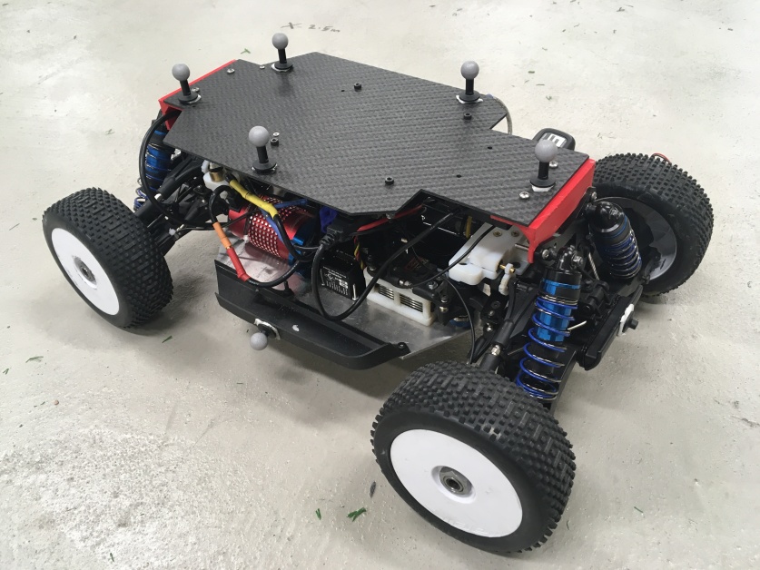
In order to verify functionality of proposed method we perform experiments on a $\frac{1}{8}^{th}$ scale, four wheel drive vehicle platform known as Parkour car (Fig.5) in a lab environment equipped with a motion capture system. Parkour car has a wheel base of $l=34\text{cm}$ and includes an on-board computer to perform all computation on the vehicle. While in action, the main computer receives a pose update from motion capture system through WiFi connection, after which a new control action is calculated based on the synthesized control law which then gets transmitted to an ECU (Electronic Control Unit). The ECU handles signal conditioning for acceleration and steering motors on Parkour car. One iteration of this control action calculation can be performed in less than $300\mu\text{s}$ on a single CPU core running at 3.5GHz. The low computation cost makes this method attractive for real-time applications aboard platforms with low computation capabilities.

Straight Path:

Solid (dashed) lines are simulation trajectories corresponding to PF-CF (TT-CF). Blue (red) trajectories start from the same initial condition.

Figure 6: Simulation Results for a Straight Path

In the first experiment, we consider a straight path from $x=-2$ to $x=2$ with the reference trajectory $\mathbf{x}_{r}(t):[-\pi/2,-2+2t,0,2]^{\intercal}$. The sets are

$$S(\theta):[-1,1]^{3}\times[-3,3]\,,\,I:\mathcal{B}_{0.5}\,,\,G:\mathcal{B}_{0.5}\,,$$

where $\mathcal{B}_{r}$ is a ball of radius $r$ centered at the origin. The learning framework then successfully finds a PF-CF. However, the learning framework fails to find a TT-CF. This does not rule out the existence of a TT-CF, however. Next, we increase the length of the path to $8\text{m}$ (from $x=-4$ to $x=4$). In this case, the learning framework can find a TT-CF. Fig. 6 shows simulation trajectories corresponding to the PF-CF and the TT-CF. For comparison, starting from the same initial conditions, the simulation is performed until $x$ reaches $x(0)+12$. Fig. 6(a) shows the results for initial states where the initial state is near $I$. The simulations suggest that both methods perform similarly and all trajectories converge to the path ($y$ converges to zero). The simulation time for all cases are similar and around $6\text{s}$. Also, the velocity of the vehicle is almost constant for both methods. Fig. 6(b) shows the results for cases when the initial states are further away from $G$ (it needs more forces/time to reach $G$). In this case, the path-following method takes a longer time to reach $x=4$ as the speed increases smoothly. Fig. 6(c) considers initial states that are closer to $G$. For these case, the path-following method takes a shorter time to reach $x=12$ as the speed decreases smoothly. The results demonstrate that the path-following method yields a faster convergence to the reference path. Moreover, the velocity changes smoothly while the trajectory tracking method settles the target velocity immediately.

We also investigate the same problem (straight path from $x=-4$ to $x=4$) where the velocity is more restricted:

$$S(\theta): [-1,1]^{3}\times[-0.5,0.5]$$

$$I:G: \{\mathbf{x}|4\alpha^{2}+4x^{2}+4y^{2}+16v^{2}\leq 1\}\,.$$

Again, under these circumstances, learning TT-CF fails while finding PF-CF is feasible. In other words, in trajectory tracking the change of velocity is crucial for reducing the tracking error.

Circular Path

To carry out experiments on Parkour car and examine the behavior over long trajectories, we consider a circular path with radius $1.5\text{m}$. The vehicle moves with a constant velocity $\frac{\pi}{2}m/s$ and the reference trajectory would be $\mathbf{x}_{r}(t):[\frac{\pi}{3}t,1.5\cos(t),1.5\sin(t),\frac{\pi}{2}]^{t}$. For the learning process, we consider a finite trajectory (once around the circle) where $t\in[0,6]$. The sets are:

$$S(\theta):[-1,1]\times[-3,3],\ I:\mathcal{B}_{0.5},\ G:\mathcal{B}_{0.5}\,.$$

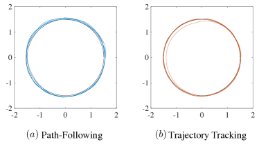
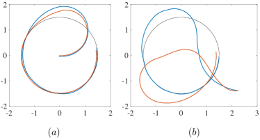
Figure 7 shows the trajectories when the controller runs on Parkour car. Despite the uncertainties in the measurements and simple modeling, both controllers do a good job of following the reference path. Fig. 8 shows the trajectories for different initial states. Fig. 8(b) suggest that the trajectory tracking method may take shortcuts to satisfy time constraints.

Figure 7: Projection of trajectories, generated on Parkour car, for the circular path. Parkour car finishes five rounds around the circle. The reference trajectory is shown in black.

Figure 8: projection of trajectories, generated on Parkour car, for the circular path form different initial states. Blue (red) lines corresponds to the path-following (trajectory tracking) method. The reference trajectory is shown in black. Initial state: (a) $[-\pi/2,0,0,0]$ and (b) $[\pi,2.25,-1.4,0]$.

We also investigated the same problem with higher reference velocity. When the reference velocity is increased to $\pi$ (from $\pi/2$), we could not find a TT-CF. Nevertheless, increasing reference velocity does not seem to affect the process of finding PF-CF, and we can discover solutions even if the reference velocity is $10\pi$.

Oval Path:

Following a circular path is easy as the curvature remains fixed. However, the problem is more challenging when the path is an oval. The goal is to follow an oval path $P:\{\frac{y^{2}}{1^{2}}+\frac{x^{2}}{2^{2}}=1\}$. First, a reference trajectory is generated to follow this path closely. As polynomial approximations of the reference path become more challenging, we divide the reference path into two similar parts. Then, we find a funnel for each part and make sure we can concatenate these two funnels. For the first part, the goal is to reach from $\mathcal{B}_{0.5}([2,0])$ to $\mathcal{B}_{0.5}([-2,0])$ going in a CCW direction and then reach from $\mathcal{B}_{0.5}([-2,0])$ to $\mathcal{B}_{0.5}([2,0])$ again in a CCW direction. For both segments we use the following sets:

$$S(\theta):[-1,1]\times[-3,3],\ I:\mathcal{B}_{0.5},\ G:\mathcal{B}_{0.5}\,.$$

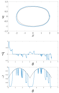
Notice that since $G$ for the first segments fits in $I$ for the second segment, we can safely concatenate the funnels. If a trajectory tracking method is being used, the learning procedure fails to find solutions. However, the path following method yields proper control funnels. Figure 9 shows the trajectories generated from our experiments using the CF-based controller. The tracking is not precise when the curvature is at its maximum. We believe the main reason is input saturation for the steering, which occurs because of the imprecise model we use (Fig. 9).

Figure 9: Projection of the trajectory, generated on Parkour car, for the oval path. The reference trajectory is shown in black.

Obstacle Avoidance:

Going back to the scenario of obstacle avoidance, we wish to find a control funnel to guarantee safety (avoiding the obstacle). Having a reference trajectory, instead of defining $S(\theta)$, we simply define $S$ as

$$S:\ \{\mathbf{x}\ |\ ([x,y]\oplus\mathcal{B}_{0.25})\cap O=\emptyset\}\,,$$

where $O$ is the obstacle, $\oplus$ is the Minkowski sum, and $0.25m$ is the distance between the center of the car and its corners (the body of Parkour car fits in $\mathcal{B}_{0.25}$). This trick allows to reason only about the center of the car, and safety is guaranteed as long as the center of the car is in $S$. Next, we set $I:\mathcal{B}_{0.25}$ and $G:\mathcal{B}_{0.25}$. However, we can not find a solution using the learning framework. To relax the conditions, we allow $G$ to be larger $G:\mathcal{B}_{0.5}$. In this case, we were able to find a solution (only if the path-following method is being used). For the experiment, Parkour car moves toward the obstacle with different initial states and the CF-based controller engages when the car is $1.5m$ to the left or right of the obstacle’s $x$ position. Fig. 10 shows the projection of the funnel on $x$-$y$ plain. We note that if a trajectory starts from the head of the funnel, not only its initial $x$ and $y$, but also its initial $v$ and $\alpha$ should also be inside the funnel. Fig. 10 (a) shows trajectories where the initial state is inside the head of the funnel. As shown, the trajectories remain inside the funnel and reach the tail. However, as demonstrated in Fig. 10 (b), even if the trajectory starts outside of the funnel head, the whole body of the car may remain in the guaranteed region (blue region). Nevertheless, the safety is not guaranteed any longer as Fig. 10 (c) shows trajectories where Parkour car leaves the guaranteed region.

Figure 10: Projection of trajectories on $x--y$ plane generated by Parkour car for the obstacle avoidance problem. Funnel boundary is shown in gray and as long as the center of car is in the funnel, the whole body of the car remains in the blue region. (a) guaranteed traces, (b) not guaranteed but safe traces, (c) not guaranteed and unsafe traces.

VI CONCLUSIONS

In this work, we investigate the use of control Lyapunov functions for path following and provide a characterization of control funnel functions for tracking a trajectory segment. Our approach lends itself to an efficient synthesis technique presented previously. We implement the resulting controller on the Parkour car and show its effectiveness through a set of tracking problems. Future work will focus on integrating our approach more closely with planning approaches to augment existing approaches to the synthesis of control funnels [34].

References

- [1] J. Hauser and R. Hindman, “Maneuver regulation from trajectory tracking: Feedback linearizable systems*,” IFAC Proceedings Volumes, vol. 28, no. 14, pp. 595 – 600, 1995.
- [2] G. J. Pappas, “Avoiding saturation by trajectory reparameterization,” in Proceedings of 35th IEEE Conference on Decision and Control, vol. 1, Dec 1996, pp. 76–81 vol.1.
- [3] M. Egerstedt, X. Hu, and A. Stotsky, “Control of mobile platforms using a virtual vehicle approach,” IEEE Transactions on Automatic Control, vol. 46, no. 11, pp. 1777–1782, Nov 2001.
- [4] M. Mason, “The mechanics of manipulation,” in ICRA, vol. 2. IEEE, 1985, pp. 544–548.
- [5] A. Majumdar, A. A. Ahmadi, and R. Tedrake, “Control design along trajectories with sums of squares programming,” in ICRA. IEEE, 2013, pp. 4054–4061.
- [6] P. Wieland and F. Allgower, “Constructive safety using control barrier functions,” IFAC Proceedings Volumes, vol. 40, no. 12, pp. 462 – 467, 2007.
- [7] H. Ravanbakhsh and S. Sankaranarayanan, “Learning lyapunov (potential) functions from counterexamples and demonstrations,” in RSS, 2017.
- [8] R. W. Brockett et al., “Asymptotic stability and feedback stabilization,” Differential geometric control theory, vol. 27, no. 1, pp. 181–191, 1983.
- [9] G. Walsh, D. Tilbury, S. Sastry, R. Murray, and J. P. Laumond, “Stabilization of trajectories for systems with nonholonomic constraints,” IEEE Trans. on Automatic Control, vol. 39, no. 1, pp. 216–222, Jan 1994.
- [10] W. L. Nelson and I. J. Cox, Local Path Control for an Autonomous Vehicle. New York, NY: Springer New York, 1990, pp. 38–44.
- [11] M. Sampei, T. Tamura, T. Itoh, and M. Nakamichi, “Path tracking control of trailer-like mobile robot,” in IROS’91, 1991, pp. 193–198 vol.1.
- [12] C. C. de Wit and R. Roskam, “Path following of a 2-dof wheeled mobile robot under path and input torque constraints,” in ICRA, 1991, pp. 1142–1147.
- [13] C. Samson, “Path following and time-varying feedback stabilization of a wheeled mobile robot,” in Intl. Conf. Advanced Robotics and Computer Vision, vol. 13, 1992, p. 1.
- [14] O. J. Sordalen and C. C. de Wit, “Exponential control law for a mobile robot: extension to path following,” IEEE Trans. on Robotics and Automation, vol. 9, no. 6, pp. 837–842, Dec 1993.
- [15] D. R. Nelson, D. B. Barber, T. W. McLain, and R. W. Beard, “Vector field path following for miniature air vehicles,” IEEE Trans. on Robotics, vol. 23, no. 3, pp. 519–529, June 2007.
- [16] D. Lawrence, E. Frew, and W. Pisano, “Lyapunov vector fields for autonomous UAV flight control,” in AIAA Guidance, Navigation and Control Conference and Exhibit, p. 6317.
- [17] T. Faulwasser and R. Findeisen, Nonlinear Model Predictive Path-Following Control. Springer, 2009, pp. 335–343.
- [18] T. Faulwasser, J. Matschek, P. Zometa, and R. Findeisen, “Predictive path-following control: Concept and implementation for an industrial robot,” in 2013 IEEE International Conference on Control Applications (CCA), Aug 2013, pp. 128–133.
- [19] P. Encarnacao and A. Pascoal, “Combined trajectory tracking and path following: an application to the coordinated control of autonomous marine craft,” in IEEE CDC, vol. 1, 2001, pp. 964–969.
- [20] R. Skjetne, T. I. Fossen, and P. V. Kokotović, “Robust output maneuvering for a class of nonlinear systems,” Automatica, vol. 40, no. 3, pp. 373 – 383, 2004.
- [21] E. D. Sontag, “A ’universal’ construction of artstein’s theorem on nonlinear stabilization,” Systems & Control Letters, vol. 13, no. 2, pp. 117 – 123, 1989.
- [22] ——, “A lyapunov-like characterization of asymptotic controllability,” SIAM Journal on Control and Optimization, vol. 21, no. 3, pp. 462–471, 1983.
- [23] W. Tan and A. Packard, “Searching for control lyapunov functions using sums of squares programming,” sibi, vol. 1, p. 1, 2004.
- [24] A. P. Aguiar, D. B. Dačić, J. P. Hespanha, and P. Kokotović, “Path-following or reference tracking?: An answer relaxing the limits to performance,” IFAC Proceedings Volumes, vol. 37, no. 8, pp. 167 – 172, 2004.
- [25] T. Faulwasser and C. M. Hackl, “Path-following funnel control for rigid-link revolute-joint robotic systems,” in Proc. MTNS’14, 2014.
- [26] M. Frego, E. Bertolazzi, F. Biral, D. Fontanelli, and L. Palopoli, “Semi-analytical minimum time solutions with velocity constraints for trajectory following of vehicles,” Automatica, vol. 86, pp. 18 – 28, 2017. [Online]. Available: http://www.sciencedirect.com/science/article/pii/S0005109817304508
- [27] S. M. LaValle, Planning Algorithms. Cambridge University Press, 2006. [Online]. Available: http://msl.cs.uiuc.edu/planning/
- [28] Z. Artstein, “Stabilization with relaxed controls,” Nonlinear Analysis: Theory, Methods & Applications, vol. 7, no. 11, pp. 1163 – 1173, 1983.
- [29] I. Lopez and C. R. McInnes, “Autonomous rendezvous using artificial potential function guidance,” Journal of Guidance, Control, and Dynamics, vol. 18, no. 2, pp. 237–241, 1995.
- [30] J. Hauser and A. Saccon, “Motorcycle modeling for high-performance maneuvering,” IEEE Control Systems Magazine, vol. 26, pp. 89–105, 2006.
- [31] A. Saccon, J. Hauser, and A. Beghi, “A virtual rider for motorcycles: Maneuver regulation of a multi-body vehicle model,” IEEE Trans. on Control Systems Technology, vol. 21, pp. 332–346, 2013.
- [32] P. Bouyer, N. Markey, N. Perrin, and P. Schlehuber-Caissier, “Timed-automata abstraction of switched dynamical systems using control invariants,” Real-Time Systems, vol. 53, no. 3, pp. 327–353, 2017.
- [33] H. Ravanbakhsh and S. Sankaranarayanan, “Learning control lyapunov functions from counterexamples and demonstrations,” CoRR, vol. abs/1804.05285, 2018. [Online]. Available: http://arxiv.org/abs/1804.05285
- [34] A. Majumdar and R. Tedrake, “Robust online motion planning with regions of finite time invariance,” in Algorithmic Foundations of Robotics X. Springer, 2013, pp. 543–558.