Topics in Geometric Group Theory. Part I

Abstract

This survey paper concerns mainly with some asymptotic topological properties of finitely presented discrete groups: quasi-simple filtration (qsf), geometric simple connectivity (gsc), topological inverse-representations, and the notion of easy groups. As we will explain, these properties are central in the theory of discrete groups seen from a topological viewpoint at infinity. Also, we shall outline the main steps of the achievements obtained in the last years around the very general question whether or not all finitely presented groups satisfy these conditions.

Keywords: Geometric simple connectivity (gsc), quasi-simple filtration (qsf), inverse-representations, finitely presented groups, universal covers, singularities, Whitehead manifold, handlebody decomposition, almost-convex groups, combings, easy groups.

MSC Subject: 57M05; 57M10; 57N35; 57R65; 57S25; 20F65; 20F69.

1 Introduction

This is a two-part survey paper, part I by D. Otera and V. Poénaru, part II by V. Poénaru (to appear soon in arXiv). In this first part we present, mostly, background material, historical context, and motivations. Its main items are the theory of topological inverse-representations, a sort of dual notion to the usual group representations, some tameness conditions at infinity for open manifolds, cell-complexes and discrete groups, such as geometric simple connectivity (gsc), Dehn-exhaustibility, the qsf property, and then a glimpse into the more recent joint work of both authors on combings of groups and on the so-called Whitehead nightmare.

On the other hand, Part II is much more technical, since it outlines the proof (announced in [56] and proved in [58, 59]) that all finitely presented groups satisfy the qsf property (see also the related [57]). This highly non-trivial notion, which in a certain sense is the good extension of simple connectivity at infinity (they are actually equivalent for closed 3-manifold groups), was introduced by Brick, Mihalik and Stallings [5, 73], and it has roots in earlier work of Casson and of Poénaru [20, 51], as well as in the much older work of Max Dehn.

Note that, even for the very special class of 3-manifold groups, in order to show they all are qsf one needs deep and difficult results such as either the geometrization theorem in dimension 3 [2, 34, 35, 46, 47, 48, 77] or else the works of Agol, Haglund and Wise on special groups [1, 28].

1.1 Acknowledgments

We would like to thank the referee who helped us to greatly improve the presentation of the paper. His/her pertinent suggestions, corrections and comments gave us the opportunity to make our paper much more readable, precise, structured and complete.

2 Topology at infinity, universal covers and discrete groups

The main technical tool used in this survey is what we call a topological inverse-representation for a finitely presented discrete group $G$. We write here “representation” in capital letters, so as to distinguish it from the standard well-known group representations. But some preliminaries will be necessary before we can actually define our representations of groups.

2.1 The $\Phi/\Psi$-theory and zippings

We consider some completely general non-degenerate simplicial map $f:X\to M$. Here $X$ and $M$ are simplicial complexes, $X$ being at most countable, and it is also assumed that ${\rm{dim}}(X)\leq{\rm{dim}}(M)$. But $X$ need not be locally-finite and it will be endowed with the weak topology. By definition, a singularity $x\in{\rm{Sing}}(f)\subset X$ is a point of $X$ in the neighborhood of which $f$ fails to inject, i.e. fails to be immersive.

Trivially, the map $f$ defines an equivalence relation $\Phi(f)\subset X\times X$, by $(x_{1},x_{2})\in\Phi(f)\Leftrightarrow f(x_{1})=f(x_{2})$.

We will be interested in equivalence relations on $X$, $\mathcal{R}\subset X\times X$, with the following additional feature: let $\sigma_{1},\sigma_{2}\subset X$ be two simplexes of the same dimension and such that $f(\sigma_{1})=f(\sigma_{2})$. If we can find $x_{1}\in\rm{int}\ \sigma_{1}$, $x_{2}\in\rm{int}\ \sigma_{2}$ such that $f(x_{1})=f(x_{2})$, then we also have the implication $(x_{1},x_{2})\in\mathcal{R}\Rightarrow\mathcal{R}$ identifies $\sigma_{1}$ to $\sigma_{2}$.

This kind of equivalence relations will be called $f$-admissible. Notice that, whenever $\mathcal{R}\subset\Phi(f)$ is admissible, we have a natural simplicial commutative diagram

$\left(1-1\right)$ $$\begin{diagram}$$

With this, we develop now the following little theory, for which the detailed definitions, lemmas and proofs, are to be found in [49, 57]. The point here is that, in the context of our non-degenerate simplicial map $f$, there is also another equivalence relation more subtle than the $\Phi(f)$. This is the $\Psi(f)\subset\Phi(f)\subset X\times X$, characterized by the following lemma:

Lemma 1.

([49]) There is a unique, $f$-admissible equivalence relation $\Psi(f)\subset\Phi(f)\subset X\times X$ which has the following two properties, which also characterize it.

• In the context of the corresponding commutative diagram (1 – 1), which we write again below

  $\left(1-2\right)$ $$\begin{diagram}$$

  we have ${\rm{Sing}}(f_{1})=\emptyset$, i.e. $f_{1}$ is immersive.

• Let $\mathcal{R}$ be any equivalence relation (not necessarily assumed a priori to be admissible), such that $\mathcal{R}\subset\Phi(f)$ and ${\rm{Sing}}(f_{1}(\mathcal{R}))=\emptyset$. Then $\mathcal{R}=\Psi(f)$.

In plain English, $\Psi(f)$ is the smallest equivalence relation, compatible with $f$, which kills all the singularities. We also have the next lemma, which has no equivalent for $\Phi(f)$.

Lemma 2.

([49]) In the context of (1 – 2), the following induced map is surjective:

$$\pi_{\ast}:\pi_{1}(X)\to\pi_{1}\big{(}X/\Psi(f)\big{)}.$$

Of course, nothing like Lemma 2 is true for the equivalence relation $\Phi(f)$ which, contrary to $\Psi(f)$, has no topological memory, a feature which is one of the reasons that makes $\Psi(f)$ interesting.

We will give now some ideas of how one may construct $\Psi(f)$. In order to effectively build our $\Psi(f)$, let us look now for a most efficient way of killing the singularities of $f$, in a manner which should have the minimum of collateral effects.

Start with two simplexes $\sigma_{1},\sigma_{2}\subset X$ of the same dimension, such that $f(\sigma_{1})=f(\sigma_{2})$, and with $\sigma_{1}\cap\sigma_{2}\ni x_{1}\in{\rm{Sing}}(f)$. We can go then to a first quotient space $f_{1}:X_{1}=X/\rho_{1}\to M$, that kills $x_{1}$ via the folding map which identifies $\sigma_{1}$ to $\sigma_{2}$. This is an equivalence relation $\rho_{1}\subset\Phi(f)$, and one can continue this process, with a sequence of folding maps:

$$\rho_{1}\subset\rho_{2}\subset\ldots\subset\rho_{n}\subset\rho_{n+1}\ldots\subset\Phi(f).$$

Here $\rho_{\omega}=\bigcup_{1}^{\infty}\rho_{i}$ is an equivalence relation too, subcomplex of $\Phi(f)$ (i.e. closed in the weak topology), and the following induced map

$$f_{\omega}:X/\rho_{\omega}\to M$$

is again simplicial. If $f_{\omega}$ is not immersive, we can continue to the next transfinite ordinal, with $\rho_{\omega}\subset\rho_{\omega+1}\subset X\times X$, and go to:

$$f_{\omega+1}:X/\rho_{\omega+1}\to M.$$

Now, we can continue via the obvious transfinite induction. Since $X$ is assumed to be at most countable, the process has to stop at some countable ordinal $\omega_{1}$, and one can actually show that $\rho_{\omega_{1}}=\Psi(f)$. This $\omega_{1}$ is not unique, but then we also have the following useful lemma.

Lemma 3.

([49]) One can chose our sequence of folding maps $(\rho_{i})$ so that $\omega_{1}=\omega$.

The sequence of folding maps coming with $\rho_{\omega}=\Psi(f)$ is called a zipping of $f$. This kind of zipping strategy is, of course, not unique. Towards the end of this paper, another alternative way to conceive zipping strategies will be presented too.

2.2 Geometric simple connectivity

The notion of geometric simple connectivity (gsc), which will play a big role in this survey, stems from differential topology, and was probably conceived by T. Wall [80]. A smooth manifold $M$ is said to be gsc (geometrically simply connected) if it has a handlebody decomposition without handles of index one (or, more precisely, if it possesses a smooth handlebody decomposition with a unique handle of index zero and with its 1-handles and 2-handles in cancelling position). If $M$ is closed, this can also be easily rephrased in Morse-theoretical terms. Saying that $M$ is gsc means that there exists a Morse function $f:M\to\mathbb{R}_{+}$ without singularities of index $\lambda=1$. Of course gsc can also be defined Morse-theoretically for open manifolds and for the case of non-empty boundary [50]. But then appropriate restrictions have to be added to the definition and we will not go into that here. Concerning gsc, more details are also provided in [16, 17, 38, 42, 60, 61, 64, 65].

As said above, the gsc concept also extends to open manifolds, manifolds with boundary and to cell-complexes too, and the ones of interest here will always be infinite.

Definition 1.

A cell-complex $X$ is said to be gsc if it admits a cell decomposition of the following type

$\left(1-3\right)$ $$X=T\ \bigcup\ \sum_{i=1}^{\infty}\{\mbox{1-cells }H_{i}^{1}\}\ \bigcup\ \sum_{j=1}^{\infty}\{\mbox{2-cells }H_{j}^{2}\}\ \bigcup\ \sum_{k;\lambda\geq 2}\{\lambda\mbox{-cells }H_{k}^{\lambda}\},$$

such that:

• $T\subset X$ is a properly embedded tree,

• in (1 – 3) the infinite sets of indices $\{i\}$ and $\{j\}$ are in canonical bijection and the geometric intersection matrix takes the form

  $\left(1-4\right)$ $$H_{j}^{2}\cdot H_{i}^{1}=\{\delta_{ji}+a_{ji}\in\mathbb{Z}_{+},\mbox{ where }a_{ji}>0\Leftrightarrow j>i\}.$$

  Here $H_{j}^{2}\cdot H_{i}^{1}$ is the number of times $H_{j}^{2}$ goes through $H_{i}^{1}$, without any $+$ or $-$ signs being counted. Notice that $\{H_{j}^{2}\}$ is only an appropriately chosen subset of the 2-cells $\{H_{j}^{2}\}\subsetneq\{H^{2}\}$.

Of course, the decomposition (1 – 3) also makes sense when $X$ is replaced by a smooth manifold $M^{n}$. If $M^{n}$ is open, then the $T$ in (1 – 3) becomes a ball $B^{n}\setminus\{$a closed tame subset deleted from $\partial B^{n}\}$, and “tame” means that the subset in question is contained inside some smooth line embedded in $\partial B^{n}\simeq S^{n-1}$; while when $M^{n}$ is compact, $T$ becomes a $B^{n}$ (a handle of index $\lambda=0$). Similarly, the various $\lambda$-cells occurring in (1 – 3), always with $\lambda>1$, become smooth $n$-handles of index $\lambda$ (and see here [57, 60, 61, 64] for more details).

Also, the condition in the right hand side of (1 – 4) will be called easy id + nilpotent. This should be distinguished from the dual condition “difficult id + nilpotent” where the inequality in (1 – 4) gets reversed into $a_{ji}>0\Leftrightarrow j<i$. Of course, in the finite case the two conditions are equivalent, but not in our infinite case of interest. For instance, the classical Whitehead manifold $Wh^{3}$ [81] (see the next section for details), always the villain in our present story, admits cell-decompositions which are of the difficult id + nilpotent type. And $Wh^{3}$ is certainly not gsc, a fact which is connected to the $\pi_{1}^{\infty}Wh^{3}\neq 0$, as we shall see.

Here is now a useful related definition which is a sort of weakening of the gsc, specific for the non-compact case, due to L. Funar [16, 17].

Definition 2.

An infinite cell-complex $X$ is said to be weakly geometrically simply connected (wgsc) if it admits an exhaustion by compact and simply-connected sub-complexes $X=\bigcup_{i=1}^{\infty}K_{i}$, where $K_{1}\subset K_{2}\subset\ldots\subset K_{j}\subset\ldots\subset X$ and $\pi_{1}(K_{i})=0$ for all $i$’s.

Clearly gsc $\Rightarrow$ wgsc and in the compact case wgsc becomes mere simple-connectivity. One may also notice that, while gsc has close ties with the all-important notion of “collapsibility”, there is nothing like that for wgsc.

Finally, we remind the reader of another fundamental tameness condition at infinity for open manifolds. A locally compact and simply connected space $X$ is said to be simply connected at infinity (and one will write $\pi_{1}^{\infty}X=0$) if for every compact $k\subset X$ there is a larger compact subset $k\subset K\subset X$ such that the induced map $\pi_{1}(X-K)\to\pi_{1}(X-k)$ is zero.

The simple connectivity at infinity is a very strong asymptotic notion and in fact, it has been used to detect Euclidean spaces among open contractible manifolds, by results of Siebenmann and Stallings in dimension at least 5 [69, 70], Freedman in dimension 4 [13], and Edwards and Wall in dimension 3 [11, 79] (see [38] for a general overview). Note also that the notion $\pi_{1}^{\infty}=0$ also makes sense for finitely presented groups [3, 75]. An old classical easy fact specific for dimension three is the following one: an open 3-manifold $V^{3}$ which is wgsc is also simply connected at infinity (see e.g. [44]). In higher dimension ($n\geq 5$), it turns out that open simply connected $n$-manifolds which are also simply connected at infinity are actually gsc [64].

M. Davis [9] exhibited, in any dimension at least 4, the first examples of fundamental groups of aspherical closed manifolds which are not simply connected at infinity, while in dimension 3, all finitely presented (3-manifold) groups are simply connected at infinity, as a consequence of Thurston geometrization conjecture [77] proved by Perelman’s work [2, 34, 35, 46, 47, 48] (this also follows by Agol’s proof of the virtually Haken Conjecture [1] and by the work of Haglund-Wise on special groups [28]).

2.3 The Whitehead manifold

Before going on, let us say few words about the renowned Whitehead 3-manifold $Wh^{3}$ and its cell-decompositions. This manifold is the main example of an open 3-manifold which is contractible but not homeomorphic to the Euclidean space $\mathbb{R}^{3}$ (see for instance [37, 81]); in particular, the manifold $Wh^{3}$ is homotopically equivalent to a point but is not tame (which means that it is not homeomorphic to a compact manifold with a closed subset of the boundary removed, see e.g. [1, 32, 78]).

This interesting manifold was discovered by J.H.C. Whitehead around 1934 ([81]), actually as a counterexample to his attempted proof of Poincaré Conjecture. Roughly speaking, its construction goes as follows: take a solid torus $T_{1}\subseteq\mathbb{R}^{3}$, and embed a thinner torus $T_{2}$ inside $T_{1}$ so that it links with itself (or, in other simple words, so that it embeds as a Whitehead link, see e.g. [16, 19]). Now, iterate the process in such a way that, at each step, one embeds a solid torus $T_{i}$ inside $T_{i-1}$, like $T_{2}$ is embedded inside $T_{1}$, obtaining an infinite sequence: $T_{1}\supset T_{2}\supset\cdots T_{i}\supset\cdots$. The Whitehead continuum is the intersection of all the tori $T_{i}$, and the Whitehead manifold $Wh^{3}$ is the complement of it in the three-sphere $\mathbb{S}^{3}$. In a dual way, $Wh^{3}$ can be also described as being the ascending union of solid tori $T_{j}$ embedded inside $T_{j+1}$ so that $T_{j}$ is a Whitehead link in the interior of $T_{j+1}$ (and this is the classical description of $Wh^{3}=\bigcup_{1}^{\infty}T_{j}$ ). See here Figure 1 and [61, 63].

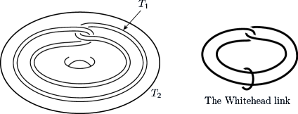
Figure 1: The Whitehead manifold $Wh^{3}$ and the Whitehead link.

The main features of the Whitehead manifold are that $Wh^{3}$ is not simply connected at infinity (intuitively, this means that there are loops at infinity that cannot be killed staying close to infinity) and that the product $Wh^{3}\times\mathbb{R}$ is actually diffeomorphic to the standard $\mathbb{R}^{4}$ (this result was first showed by Shapiro and Glimm, and see here [22] where it is also proved that the Cartesian product of the Whitehead manifold with itself is topologically $\mathbb{R}^{6}$). Moreover, recently, D. Gabai has also demonstrate a surprising result: the Whitehead manifold can be described as the union of two embedded submanifolds, both homeomorphic to $\mathbb{R}^{3}$, and such that their intersection is also homeomorphic to $\mathbb{R}^{3}$ (see [19]).

What is interesting for us here is that although $Wh^{3}$ is not gsc (since this would imply $\pi_{1}^{\infty}Wh^{3}=0$, see the comment just after Lemma 5), it still admits handlebody decompositions with geometric intersection matrix of the form difficult id + nilpotent, as outlined in [61].

For instance, consider the Figure 2. There is there a disk whose boundary is a curve $T_{1}$, so that the disk intersects itself, and the intersection is a double line (denoted, in the picture, by $[b,c]$). This is a 2-dimensional object that leads to a handlebody decomposition of $S^{1}\times D^{2}$, whose geometric intersection matrix is $H_{1}^{2}\cdot H_{1}^{1}=1$ and $H_{1}^{2}\cdot H_{2}^{1}=2$. More precisely this means that there is only one 0-handle, two 1-handles and one 2-handle, and the double line $[b,c]$ of above is $H_{2}^{1}$. To go on, one takes now another closed loop which goes through both a piece of $T_{1}$ and $H^{1}_{2}$, and next one deals with this loop like we have just done with the curve $T_{1}$, i.e. by adding along it another disk which hits itself back. Once again, this process leads to another handlebody decomposition of $S^{1}\times D^{2}$, whose geometric intersection matrix takes now the form $H_{1}^{2}\cdot H_{1}^{1}=1$, $H_{1}^{2}\cdot H_{2}^{1}=2$, and $H_{2}^{2}\cdot H^{1}_{2}=1$, $H^{2}_{2}\cdot H^{1}_{3}=2$.

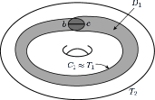
Figure 2: Disks inside $Wh^{3}$.

This procedure can continue indefinitely, getting an infinite matrix which is of the form difficult id + nilpotent. But the problem is that the resulting object is not our manifold $Wh^{3}$ (since it is 2-dimensional and it is even not locally-finite).

However, one can cleverly manipulate the process in order to get the desired result. Firstly, after each one of the infinitely many steps, one may add additional handles of index 1, 2 and 3, in order to obtain a 3-dimensional object. Then, it can be shown that, by paying close attention to details, one can actually manage to obtain a handlebody decomposition for the Whitehead manifold which is proper (i.e. it does not accumulate at finite distance), and whose geometric intersection matrix is made of a main difficult id + nilpotent part, and of some additional easy id + nilpotent parts (which do not interfere with the main difficult part).

To conclude our digression on this interesting manifold, we outline some of the developments that have occurred since the original input given by the appearance of $Wh^{3}$. First of all, in the 60s, McMillan [31] constructed uncountably many contractible open 3-manifolds with no two homeomorphic, most of which are not universal covers of closed 3-manifolds, just because there are only countably many closed 3-manifolds and, therefore, only countably many open contractible 3-manifolds which cover closed 3-manifolds. But the first concrete examples of such manifolds (the so-called genus-one Whitehead manifolds) were constructed only afterwards in [36]: these manifolds admit no non-trivial, free, and properly discontinuous group actions, and thus they cannot cover non-trivially a non compact 3-manifold. Genus-one Whitehead manifolds are irreducible, contractible, open manifolds which are monotone unions of solid tori but are not homeomorphic to $\mathbb{R}^{3}$. The class of such examples was further enlarged by Wright in [82], where he constructed, for each $n\geq 3$, specific examples of contractible $n$-manifolds (called Whitehead-type $n$-manifolds) similar to Whitehead’s original 3-manifold (obtained, for instance, almost in the same way as $Wh^{3}$, just by considering solid $n$-tori instead of 2-dimensional ones) which cannot non-trivially cover any space. Finally, in [16], Funar and Gadgil further studied Whitehead-type $n$-manifolds (that are open, contractible and not simply connected at infinity), and proved that there are uncountably many Whitehead-type $n$-manifolds for any $n\geq 5$, and that there are uncountably many such manifolds that are not geometrically simply connected!

2.4 Dehn-exhaustibility and the QSF property

We introduce next a notion which will be very useful for us here.

Definition 3.

A smooth open $n$-manifold $M^{n}$ is said to be Dehn-exhaustible if for every compact subset $k\subset M^{n}$ we can find a compact bounded $n$-manifold $K^{n}$ with $\pi_{1}K^{n}=0$ , entering in the following commutative diagram

$\left(1-5\right)$ $$\begin{diagram}$$

which is such that

• $i$ is the canonical inclusion and $j$ is an inclusion too,

• $f$ is a smooth immersion,

• the following so-called Dehn-condition is fulfilled:

  $\left(1-6\right)$ $$j(k)\cap M_{2}(f)=\emptyset,$$

  where $M_{2}(f)$ is the set of points $x\in K^{n}$ such that ${\rm{card}}\{f^{-1}f(x)\}>1$.

N.B. We will also need the related set of double points $M^{2}(f)\subset K^{n}\times K^{n}$, where $M^{2}(f)$ is the set of points $(x_{1},x_{2})\in K^{n}\times K^{n}$ such that $x_{1}\neq x_{2}$ and $f(x_{1})=f(x_{2})$. This set comes with an obvious projection on the first factor $K^{n}\times K^{n}\supset M^{2}(f)\to M_{2}(f)\subset K^{n}$.

There is quite some history behind this Definition 3. In the nineteen-twenties, when topology was in its infancy, Max Dehn published a paper, a lemma of which had the following quite striking corollary: “A knot $i:S^{1}\hookrightarrow\mathbb{S}^{3}$ is unknotted if and only if $\pi_{1}(\mathbb{S}^{3}-i(S^{1}))=\mathbb{Z}$”. In the old days, this was called “the fundamental theorem of knot theory”, and with Papakyriakopoulos’ “sphere theorem”, there is also an analogous result for links in $\mathbb{S}^{3}$.

But few years later it happened that the proof of the lemma in question, called after that “Dehn’s lemma”, was shown to be irreparably wrong. Then, in the nineteen-fifties came the big breakthrough of Papakyriakopoulos, who not only proved Dehn’s lemma [45] but, in the same breath proved the sphere theorem. This opened the first mature period of 3-manifold topology before the Thurston revolution and its sequels appeared on the scene. One should also mention that a much more transparent version of the proof of Dehn’s lemma was provided by Shapiro and Whitehead [67].

But then, a bit later, while trying, in depth, to understand what was going on in the sphere theorem, John Stallings was lead to his own theorem: “A torsion-free group with infinitely many ends is a free product” [71, 72], one of the big classical results in geometric group theory. And to finish this little historical prentice, Misha Gromov gave a very short crisp proof of Stallings theorem, using minimal surfaces [23].

Also, a few years after the appearance of [50] , Brick and Mihalik [5] abstracted the notion qsf (meaning quasi-simple filtration) from the earlier work of Casson [20] and of the second author (V.P.) [50, 51], running as follows:

Definition 4.

A locally-compact simplicial complex $X$ is said to be qsf (quasi-simply filtered) if for any compact subcomplex $k\subset X$ there is a simply-connected compact (abstract) complex $K$ endowed with an inclusion $k\overset{j}{\longrightarrow}K$ and with a simplicial map $K\overset{f}{\longrightarrow}X$ satisfying the Dehn-condition $M_{2}(f)\cap j(k)=\emptyset$, and entering in a commutative diagram like (1 – 5) above (but now with a map $f$ which is no longer an immersion, but just a simplicial map).

In other words, a locally finite simplicial complex $X$ is qsf if it satisfies something like the Dehn-exhaustibility, with the condition on $f$ relaxed from immersion to $f$ being a mere simplicial map (see here [5, 17, 38, 73]). Most of the good virtues of the Dehn-exhaustibility are preserved for the more general qsf, like for instance the implication

$\left(1-7\right)$ $$V^{3}\mbox{ open, irreducible and {qsf}}\Longrightarrow V^{3}\simeq\mathbb{R}^{3}.$$

But what one gains is very valuable, since, unlike Dehn-exhaustibility, the qsf property turns out to be a group theoretical, presentation-independent notion: if $K_{1},K_{2}$ are two presentations (i.e. two presentation complexes) for the same finitely presented group $\Gamma$, then $\widetilde{K}_{1}\in\mbox{{qsf}}\iff\widetilde{K}_{2}\in\mbox{{qsf}}$ [5].

Definition 5.

If that happens, we say that the group $\Gamma$ itself is qsf.

Now, in order to better perceive all the previously defined notions, we list several examples of spaces and groups which satisfy or do not satisfy these conditions. Of course, Euclidean spaces are the easiest examples of spaces which are simply connected at infinity (in dimension $\geq 3$), gsc, wgsc, Dehn-exhaustible and qsf. On the other hand, as already said, the Whitehead manifold $Wh^{3}$, genus-one Whitehead manifolds and Whitehead-type $n$-manifolds are examples of open manifolds which are not simply connected at infinity nor gsc nor qsf (but they are wgsc). A funny example of a simplicial complex which is qsf but not wgsc is the universal cover of the 2-complex associated to the following presentation of $\mathbb{Z}=\langle a,b|baba^{-1}b^{-1}\rangle$ (see Figure 3). In the 80s M. Davis [9] constructed the very first examples of (high-dimensional) compact aspherical manifolds (and finitely presented groups) whose universal covering spaces are not simply connected at infinity; on the other hand (most of) these compact manifolds have hyperbolic or CAT(0) fundamental groups, and so Davis’ examples are wgsc (and hence qsf). The striking result by the second author (V.P.), announced in [56] and proved in [57, 58, 59], states that actually all finitely presented groups are qsf (for easier, direct but partial results which concern just specific geometric classes of finitely presented groups that are qsf see [5, 17, 32, 73]).

Figure 3: A presentation 2-complex for $\mathbb{Z}=\langle a,b|baba^{-1}b^{-1}\rangle$, and its universal covering space, a qsf space that is not wgsc. In fact, in the process of killing any loop $b$ of the universal cover, one always creates another loop which can be killed by creating another loop, indefinitely.

2.5 On Dehn’s lemma

So, we go back now to Dehn’s lemma. In a modernised form, it can be stated as follows, and for a proof see [50].

Lemma 4 (Dehn’s lemma à la Po, [50]).

Any open simply-connected 3-manifold $V^{3}$ which is Dehn-exhaustible, is also wgsc, and hence simply connected at infinity too.

Note that the classical Dehn’s lemma says that if an embedding $S^{1}\subset M^{3}$ extends to a map $f:D^{2}\to M^{3}$ which satisfies the Dehn-condition $S^{1}\cap M_{2}(f)=\emptyset$, then $S^{1}$ is unknotted in $M^{3}$. Our Definition 3 stems from these things.

Next, here is how Dehn-exhaustibility and gsc come together. The result we will present now, as such, is unrelated to group theory. But then, on the one hand, things like it will be used later in this survey in order to prove group-theoretical results. On the other hand, it should serve as an easy paradigm of how the $\Phi/\Psi$-manipulation can be used, particularly in group theory.

For the sake of the simplicity of exposition, we give here the next result only for the case of open smooth manifolds, although the definition of Dehn-exhaustibility can be extended to more general contexts, and then the lemma below too. And this extension will be useful.

Lemma 5 (Stabilization Lemma).

Let $M^{n}$ be an open smooth manifold which is such that we can find a $p\in\mathbb{Z}_{+}$ with the property that $M^{n}\times B^{p}$ is gsc. Then $M^{n}$ is Dehn-exhaustible, with, in the context of diagram (1 – 5), a smooth $K^{n}$ and a smooth immersion $f$.

For $n=3$, the complete proof of Lemma 5 is given in [50]. But the arguments extend easily to Lemma 5 itself. We will present this below, after we open a prentice.

Notice, first, that Lemma 5 implies that when it comes to the Whitehead manifold $Wh^{3}$, then for any $p\in\mathbb{Z}_{+}$ we cannot have $Wh^{3}\times B^{p}$ gsc because, in this case, combining Lemma 4 and Lemma 5 we would get that $\pi_{1}^{\infty}Wh^{3}=0$, which is false. But then $Wh^{3}$ itself cannot be gsc either.

Another comment is that we can extend Definition 3 to a cell-complex context.

Definition 6 (Definition 3 extended).

Let $M^{n}$ be a simplicial complex which is pure, i.e. each simplex $\sigma^{\lambda}$, with $\lambda<n$, is face of a simplex $\sigma^{n}\subset M^{n}$. We say that $M^{n}$ is Dehn-exhaustible if for every compact subcomplex $k\subset M^{n}$ there is a commutative diagram

$\left(1-8\right)$ $$\begin{diagram}$$

where $K^{n}$ is a compact simply-connected pure complex, $f$ a simplicial immersion and the Dehn-condition $j(k)\cap M_{2}(f)=\emptyset$ is satisfied.

Proof of Lemma 5..

(N.B. This proof, which is essentially the same as the argument in [50], extends to the context of pure complexes and of Definition 6.)

When we consider $M^{n}\times B^{p}\supset M^{n}\times\{\ast\}\simeq M^{n}$ , with $\{\ast\}=$ the center of $B^{p}$, then $M^{n}\times B^{p}$ can be endowed with a smooth triangulation, compatible with the DIFF structure, so that $M^{n}\times\{\ast\}\simeq M^{n}$ is a subcomplex. Also, because $M^{n}\times B^{p}$ is gsc, and hence wgsc, the simplicial complex $M^{n}\times B^{p}$ is exhausted by a union of compact simply-connected subcomplexes of codimension zero $Z_{1}\subset Z_{2}\subset\cdots\subset M^{n}\times B^{p}$. We move next to the $n$-skeleta $Z^{n}_{1}\subset Z^{n}_{2}\subset\cdots\subset\cup_{i}Z^{n}_{i}=Z^{n}_{\infty}=\{\mbox{the $n$-skeleton of }M^{n}\times B^{p}\}\supset M^{n}\times\{\ast\}$ (which is a subcomplex of codimension zero).

After appropriate subdivisions and perturbations, like in [50, 59], one can ask that

$\left(1-9\right)$ $$\pi_{\infty}=\pi|_{Z^{n}_{\infty}}:Z^{n}_{\infty}\to M^{n}$$

be a simplicial non-degenerate map.

In the wake of (1 – 9), we also define $\pi_{i}=\pi|_{Z^{n}_{i}}$. For each $i\leq\infty$ we have the equivalence relations $\Phi_{i}=\Phi(\pi_{i})$ and $\Psi_{i}=\Psi(\pi_{i})$. Here, for $i<\infty$, we clearly get $\Phi_{i}=\Phi_{\infty}|_{Z^{n}_{i}}$, but, generally speaking, we only have an inclusion $\Psi_{i}\subset\Psi_{\infty}|_{Z^{n}_{i}}$.

For our triangulated $M^{n}$ we have the following commutative diagram of simplicial maps, with $\overline{\pi}_{\infty}$ the analogous of $f_{1}$ from (1 – 2):

$$\begin{diagram}$$

In other words, the projection $\overline{\pi}_{\infty}$ admits a cross-section.

Notice that the map $i$ has to be bijective, since otherwise $\overline{\pi}_{\infty}$ would have singularities (i.e. it would fail to be immersive). This means that $M_{2}(\overline{\pi}_{\infty})=\emptyset$ (see Definition 3). With this, in the following commutative diagram both horizontal and vertical maps into $M^{n}$ are bijective and hence, essentially because there is a cross-section, we find that the following two equivalence relations have to coincide

$$\Phi_{\infty}=\Psi_{\infty}.$$

There is then, starting from the equality $\Phi_{\infty}=\Psi_{\infty}$, an easy “compactness argument” (see [50]) which shows that there exists a function among positive integers $\mathcal{N}:\mathbb{Z}_{+}\to\mathbb{Z}_{+}$ such that $\mathcal{N}(j)>j$, with the following property: $\Psi_{\mathcal{N}(j)}|_{Z^{n}_{j}}=\Phi_{j}$ for all $j$’s.

Fix now a compact subset $k\subset M^{n}$. There is an $i<\infty$ such that $\pi_{i}(Z_{i}^{n})\supset k$, and since $\pi_{\infty}^{-1}(\pi_{i}(Z^{n}_{i}))$ is compact too, we find some $j>i$ such that $Z_{j}^{n}\supset\pi_{\infty}^{-1}(\pi_{i}(Z^{n}_{i}))\supset\pi_{\infty}^{-1}(k)$. Our set-up is such that, whenever we have $(x_{1},x_{2})\in M^{2}(\pi_{\infty})$ and $x_{1}\in k$, then $x_{2}\in Z^{n}_{j}$. For our $j$ we go now to the $\mathcal{N}(j)>j$ introduced above, coming with $\Psi_{\mathcal{N}(j)}|_{Z^{n}_{j}}=\Phi_{j}$, and to the following sequence of maps and inclusions:

$$k\subset Z^{n}_{j}/\Phi_{j}=Z^{n}_{j}/\Psi_{\mathcal{N}}\subset Z^{n}_{\mathcal{N}}/\Psi_{\mathcal{N}}\overset{\overline{\pi}_{\mathcal{N}}}{\longrightarrow}M^{n},$$

with $\overline{\pi}_{\mathcal{N}}$ like the $f_{1}$ in (1 – 2). Here $Z^{n}_{\mathcal{N}}/\Psi_{\mathcal{N}}$ is a compact $n$-manifold which, by Lemma 2, is simply connected, and $\overline{\pi}_{\mathcal{N}}$ is immersive. We have also that $\pi_{\infty}^{-1}(k)\subset Z^{n}_{j}$ and $\Psi_{\mathcal{N}}|_{Z^{n}_{j}}=\Phi_{j}$.

This means that $k$ cannot be involved with the double points of $\overline{\pi}_{\mathcal{N}}$, i.e. $k\cap M_{2}(\overline{\pi}_{\mathcal{N}})=\emptyset$ (Dehn-condition). With this, the commutative diagram

$$\begin{diagram}$$

with $i,j$ the obvious inclusions, has all the features of (1 – 5) in Definition 3. This ends the proof. ∎

Remark 2.1.

The argument above is a paradigm for many such, occurring in our group theoretical context. And then the “compactness argument” will occur again, coming with the function $\mathcal{N}:\mathbb{Z}_{+}\to\mathbb{Z}_{+}$. It is possibly worthwhile to try to connect asymptotic properties of the function $\mathcal{N}$, like growth, with the asymptotic properties of the corresponding finitely presented group $G$.

2.6 Presentations and REPRESENTATIONS of groups

A combinatorial presentation of a finitely presented group $G$ is a given finite system of generators $g_{i}^{\pm 1}$ and relators $\mathcal{R}_{j}$ for $G$. Traditionally, to this combinatorial presentation, one attaches a geometric presentation. This is usually a finite 2-complex $K^{2}$ with one vertex and with 1-cells and 2-cells corresponding, respectively, to the $g_{1}^{\pm 1},g_{2}^{\pm 1},\cdots,g_{n}^{\pm 1}$ and $\mathcal{R}_{1}^{\pm 1},\mathcal{R}_{2}^{\pm 1},\cdots,\mathcal{R}_{p}^{\pm 1}$. Classically, the 1-skeleton of $\widetilde{K}^{2}$ is the Cayley graph of $G$.

In our present survey we will deal, mostly, with completely general finitely presented groups $G$, but we will need to be quite choosy when it comes to geometric presentations. Such presentations will always be, for us, 3-dimensional finite complexes $M^{3}(G)$ such that $\pi_{1}M^{3}(G)=G$. And since we want to be able to deal with any finitely presented group $G$, the $M^{3}(G)$ has to have singularities, by which we mean non-manifold points. Actually, $M^{3}(G)$ will be a compact singular 3-manifold with a very precise kind of singularities, the so-called “undrawable singularities” which were a lot used by the second author in earlier work, see here [18, 39, 52]. They are displayed as little shaded rectangles in Figure 4.

Figure 4: The $N^{3}(S)\subset M_{0}^{3}(G)$ is gotten by putting these three 3-dimensional pieces together. The rectangles $[\epsilon_{j},-\epsilon_{j};\epsilon_{j}^{\prime},-\epsilon_{j}^{\prime}]$, $[\epsilon_{i},-\epsilon_{i};\epsilon_{i}^{\prime},-\epsilon_{i}^{\prime}]$ in (B), (C), respectively, are glued to the ones in (A). The immortal singularity $S$ is shaded. The $\partial N^{3}(S)=S^{1}\times S^{1}-\rm{int}D^{2}$ is made up from three contributions: the half-sphere in (A) and the two curved arches occurring in (B) and (C).

Another way to describe them is the following. Start with $R_{1}^{2}=(x=0,y,z),R_{2}^{2}=(x,y=0,z)\subset\mathbb{R}^{3}=(x,y,z)$ and with their canonical half-line $\frac{1}{2}L=(x=0,y=0,z\leq 0)\subset R_{1}^{2}\pitchfork R_{2}^{2}$. We consider then the obvious map

$\left(1-10\right)$ $$f:K^{2}=R_{1}^{2}\underset{\frac{1}{2}L}{\cup}R_{2}^{2}\longrightarrow\mathbb{R}^{3},$$

which is immersive, except at its singular point $s=(0,0,0)$. This is a 2-dimensional undrawable singularity and its 3-dimensional thickening is the kind of singularity $M^{3}(G)$ possesses.

Here is a typical example of such a 3-dimensional presentation $M^{3}(G)$ of $G$. Start with a combinatorial presentation, by generators and relators of $G$, and to it we will attach a particular 3-dimensional geometric presentation which we will call $M_{0}^{3}(G)$.

Corresponding to the generators $g_{1}^{\pm 1},g_{2}^{\pm 1},\cdots,g_{n}^{\pm 1}$ we pick up a 3-dimensional handlebody of genus $n$, i.e. a smooth bretzel $T^{3}$ with $n$-holes. To the relations corresponds a generic immersion

$\left(1-11\right)$ $$\sum_{i=1}^{r}S_{i}^{1}\overset{\Upsilon}{\longrightarrow}\partial T^{3},$$

which we immediately thicken into

$\left(1-12\right)$ $$\sum_{i=1}^{r}(S_{i}^{1}\times[-\epsilon_{i},\epsilon_{i}])\overset{\Upsilon}{\longrightarrow}\partial T^{3}.$$

We can actually always slightly change the original combinatorial presentation so that for each $i$, the individual maps $\Upsilon|_{S^{1}_{i}}$ and $\Upsilon|_{S^{1}_{i}\times[-\epsilon_{i},\epsilon_{i}]}$ actually inject. This will be assumed from now on (and it will make life easier).

Finally, for each relator $\mathcal{R}_{i}$ we attach to $T^{3}$ a 2-handle $D_{i}^{2}\times[-\epsilon_{i},\epsilon_{i}]$, of attaching zone $\partial D^{2}_{i}\times[-\epsilon_{i},\epsilon_{i}]=S_{i}^{1}\times[-\epsilon_{i},\epsilon_{i}]$, along $\Upsilon|_{S^{1}_{i}\times[-\epsilon_{i},\epsilon_{i}]}$. This final object is our $M_{0}^{3}(G)$, and this will be the typical example of our geometric presentations of groups.

This object is singular and, unless $G$ is the fundamental group of a smooth 3-manifold, a very exceptional case indeed, singularities have to be there. This is how they occur. Any transversal contact

$$\Upsilon(S^{1}_{i_{1}})\pitchfork\Upsilon(S^{1}_{i_{2}})\ni x\in\Upsilon(M_{2}(\Upsilon)),i_{1}\neq i_{2},$$

gives rise to connected components of $\Upsilon(M_{2}(\Upsilon))$ (with $\Upsilon$ like in (1 – 12)), which are little squares $[-\epsilon_{i_{1}},\epsilon_{i_{1}}]\times[-\epsilon_{i_{2}},\epsilon_{i_{2}}]\subset\Upsilon(S^{1}_{i_{1}}\times[-\epsilon_{i_{1}},\epsilon_{i_{1}}])\cap\Upsilon(S^{1}_{i_{2}}\times[-\epsilon_{i_{2}},\epsilon_{i_{2}}])$. These non-manifold regions for $M_{0}^{3}(G)$, which certainly are 3-dimensional singularities of the undrawable type mentioned above, will also be called immortal singularities, so as to distinguish them from the singularities occurring in the $\Phi/\Psi$ little theory, that are non-immersive points at the source, and which we will call mortal singularities, since these singularities do get killed by the $\Psi\subset\Phi$ equivalence relation (i.e. by the zipping).

Let us be more precise at this point. The immortal singularities are points $x$ of some $n$-dimensional space $X$, where $X$ fails to be an $n$-dimensional manifold, locally; while mortal singularities are points $x\in X$ where a non-degenerate map $f:X\to Y$ fails to be immersive, locally again.

Coming back to the presentation $M_{0}^{3}(G)$, if by any means $G$ is the fundamental group of a closed (or just compact) 3-manifold $M^{3}$, then we will take as $M_{0}^{3}(G)$ the smooth $M^{3}$ itself.

The $M_{0}^{3}(G)$ described above is an instance of what we will call a singular handlebody $P^{n}$ (for $n\geq 3$). Such an object is, by definition, a union of $n$-dimensional handles of index $\lambda=0,1,2,\cdots,n$, call them generically $h^{\lambda}=B^{\lambda}\times B^{n-\lambda}$. They have attaching zones $\partial_{a}h^{\lambda}\subsetneq\partial h^{\lambda}$, defined by $\partial_{a}h^{\lambda}=\partial B^{\lambda}\times B^{n-\lambda}$ and lateral surfaces $\delta h^{\lambda}=B^{\lambda}\times\partial B^{n-\lambda}$. These handles $h^{\lambda}$ are put together into $P^{n}$, according to the following rules of the game:

1. as usual, $\partial_{a}h^{\lambda}$ is glued to the free part of $\underset{\mu<\lambda}{\cup}\partial h^{\mu}$;

2. but we allow now for non-trivial intersections $\partial_{a}h^{\lambda}_{i}\cap\partial_{a}h^{\lambda}_{j}$, for $i\neq j$ and $\lambda\geq 1$.

This creates singularities, of a more general type than the undrawable ones.

The $M_{0}^{3}(G)$ are only one class of group-presentations, but, for technical reasons, another class, the “good-presentations”, will soon have to be introduced too. There are good reasons, as we shall see, to use our present 3-dimensional geometric presentations of $G$, rather than the classical 2-dimensional presentations.

We are finally ready to introduce the representations of $G$ (for convenience, we will skip from now on the terms “topological” and “inverse”) . The $G$ will invariably be for us a finitely presented group of the most general type.

Definition 7.

Start with an arbitrary geometric presentation of a finitely presented group $G$, $M^{3}(G)$ and go then to its universal covering space $\widetilde{M^{3}(G)}$. A representation of $G$ is a non-degenerate simplicial map

$\left(1-13\right)$ $$X^{p}\overset{f}{\longrightarrow}\widetilde{M^{3}(G)}$$

where:

• the space $X^{p}$ is a cell-complex of dimension $p=2$ or $3$ which is not necessarily locally finite, but which is geometrically simply connected (gsc). [Notice that since the map $f$ is non-degenerate, we must have $p\leq 3$; but the case $p=1$ is of absolutely no interest. According to the cases $p=2$ or $p=3$, we will talk about $2$-dimensional or $3$-dimensional representations, and both are important for us].

• $\Psi(f)=\Phi(f)$.

• The map $f$ is “essentially surjective”, which means the following. If $p=3$, then for the closure of the image we have $\overline{f(X^{3})}=\widetilde{M^{3}(G)})$; while if $p=2$, it means that $\widetilde{M^{3}(G)}$ can be gotten from $\overline{f(X^{3})}$ by adding cells of dimensions $\lambda=2$ and $\lambda=3$.

Note that, in the context of a 2-dimensional representations of $G$, $f:X^{2}\to\widetilde{M^{3}(G)}$, we may have immortal singularities of $\widetilde{M^{3}(G)}$ and, for $X^{2}$, both mortal and immortal singularities $x\in X^{2}$. In this last case, in the context of the present paper, the following things will always happen.

• At a singular $x\in X^{2}$, whether immortal or mortal, locally at $x$, our $X^{2}$ is like in (1 – 10), namely of the form $R_{1}^{2}\underset{\frac{1}{2}L}{\cup}R_{2}^{2}$ which we call an “undrawable singularity”, for obvious reasons. (This is a terminology introduced long ago by Barry Mazur, during some lengthly discussions with the second author).

• Locally, at any immortal singularity $x\in X^{2}$, the map $f$ embeds and we have $f(x)\in\{$some immortal singularity of $\widetilde{M^{3}(G)}\}$.

Remark 2.2.

• According to Misha Gromov, groups are geometric objects defined up to quasi-isometry [23, 25]. From this viewpoint, $G$ and $\widetilde{M^{3}(G)}$ are the same object, certainly the same object up to quasi-isometry. And with this, let us notice that while mundane group representations are arrows of the form $\{G\to\cdots\}$, going homomorphically into some other group, our representations take just the dual form $\{\cdots\to G\}$. And actually this is why they are called “inverse-representations”. But, as a matter of taste, we prefer the capital letters to the adjective “inverse”.

• We will also introduce a slightly weaker notion, the wgsc-representations. One proceeds exactly like in Definition 7, but simply replaces the gsc condition by wgsc.

• In very simple words a representation is a sort of resolution of the universal cover of a presentation of $G$ in the realm of cell complexes which are gsc (or wgsc).

• The reader may also have noticed that the group structure does not play any role in Definition 7, as such. But then our definition opens the door for the following possibility, which will be all-important for the more serious applications. We may have equivariant representations, where, besides the obvious action $G\times\widetilde{M^{3}(G)}\to\widetilde{M^{3}(G)}$, we also have a second free action $G\times X^{p}\to X^{p}$ such that for each $x\in X^{p}$ and $g\in G$, we should have the equivariance condition: $f(gx)=gf(x)$.

  Such equivariant representations are very useful, but they are hard to get. We will come back to them soon.

• But, once the group structure of $G$ does not play any role in Definition 7, we may also represent other 3-dimensional objects, not connected to any symmetry group

  $$X^{p}\longrightarrow Y^{3}$$

  and then $Y^{3}$ may or may not be a 3-manifold. Anyway, the existence of the representation above, forces that we should necessarily have (and see here Lemma 2) $\pi_{1}Y^{3}=0$.

  In this context, in [63] it is shown that when we represent the Whitehead manifold $Wh^{3}$, then quite naturally the Julia sets from the dynamics of quadratic maps pop up, raising of course the issue of a possible connection between wild topology and dynamical systems (for more details see the last section).

2.7 Good-presentations of finitely presented groups

We introduce now the good-presentations $M^{3}(G)$ of $G$. These will have the very useful feature that not only are $M^{3}(G)$, $\widetilde{M^{3}(G)}$ singular handlebodies, but they also admit representations $X^{3}\to\widetilde{M^{3}(G)}$, where $X^{3}$ itself is such a singular handlebody, and hence the non degenerate map $f$ sends, isomorphically, $\lambda$-handles into $\lambda$-handles, a very useful feature indeed.

To construct such good-presentations $M^{3}(G)$ we start with our previous $M_{0}^{3}(G)$, which was directly related to a given combinatorial presentation of $G$.

Let $S$ be any individual immortal singularity of $M^{3}(G)$, a little shaded square like in Figure 4. This $S$ has a canonical neighbourhood $N^{3}(S)\subset M^{3}(G)$, the detailed structure of which is shown in Figure 4 and which is split from the rest of $M^{3}_{0}(G)$ by a surface of genus one, namely by

$$\partial N^{3}(S)=S^{1}\times S^{1}-\overset{\circ}{D^{2}}.$$

[N.B.: By $\partial N^{3}(S)$ we mean here not the whole boundary, but a piece of it, the splitting locus].

We will break now $M^{3}_{0}(G)$ into a union of smaller pieces than the initial handles, but which are subcomplexes of $M^{3}_{0}(G)$

$\left(1-14\right)$ $$M^{3}_{0}(G)=\bigcup_{1}^{q}\Delta_{i}^{3}(0).$$

These $\Delta^{3}_{i}(0)$’s are supposed to have disjoined interiors. For each singularity $S$, the $N^{3}(S)$ itself is a $\Delta^{3}_{i}(0)$. All the others are copies of $B^{3}$, contained now inside a given handle, each. These smooth $\Delta^{3}_{i}(0)$’s come with $\rm{int}\Delta^{3}_{i}(0)\cap\partial(\mbox{handle})=\emptyset$, something which the singular $N^{3}(S)$’s violate.

The important thing is that, in the context of (1 – 14) the following condition is fulfilled: whenever $\rm{dim}(\Delta^{3}_{i}(0)\cap\Delta^{3}_{j}(0))>1$, then we also have

$$\partial\Delta^{3}_{i}(0)\cap\partial\Delta^{3}_{j}(0)=\{\mbox{a {unique} 2-cell }\xi\},\mbox{called a {{face}}}.$$

This is what we have gained when we refined the singular handlebody decomposition of $M^{3}_{0}(G)$, in its original description, into (1 – 14). We proceed next via the following steps:

• We triangulate, compatibly, the $\Delta^{3}_{i}(0)$’s and their common faces $\xi$. From this, we retain now only the 2-skeleta $(\Delta^{3}_{i}(0))^{(2)}$, $\xi^{(2)}$.

• Each of the 2-dimensional complexes $(\Delta^{3}_{i}(0))^{(2)}$, $\xi^{(2)}$ is changed back into a singular handlebody, via the standard procedure below:

  $$\{\lambda\mbox{-dimensional simplex}\}\to\{3\mbox{-dimensional handles of index }\lambda\}.$$

  The $(\Delta^{3}_{i}(0))^{(2)}$, $\xi^{(2)}$ become now 3-dimensional singular handlebodies denoted respectively by $\Delta^{3}_{i}$ and $g^{3}$. We may assume each $\Delta^{3}_{i}$, $g^{3}$ to be gsc and, when this is the case, $g^{3}\subset\Delta^{3}_{i}$ is now “sub-handlebody”, the meaning of this term should be obvious.

• We can glue now together the $\Delta^{3}_{i}$, $g^{3}$’s following the prescription given by (1 – 14). The result is, by definition, our good presentation of $M^{3}(G)$ (or one of such).

When the opposite is not explicitly said, our group presentations will always be good, in the text which follows.

2.8 Some historical remarks

Representations of topological spaces were already present at an intuitive level of the initial step in the approach of the second author to Poincaré Conjecture (see [18] and, for a complete up-to-date overview, see [55]). In the papers [52, 65] homotopy 3-spheres $\Sigma^{3}$ and open 3-manifolds were represented. It is actually in [52], under a different name, that representations first appeared (see also [54]).

Without giving all details, let us state the first “representation-result” from [52] (the so-called “Collapsible Pseudo-Spine Representation Theorem”):

Theorem 1 (V. Poénaru, [52]).

Given a homotopy $3$-sphere $\Sigma^{3}$, one can construct a representation $f\colon K^{2}\to\Sigma^{3}$, where $K^{2}$ is a finite $2$-complex and $f$ a non-degenerate simplicial map with undrawable singularities, like in (1 – 10), such that the complement of $f(K^{2})$ is a finite collection of open $3$-cells, $K^{2}$ is collapsible and $\Psi(f)=\Phi(f)$.

Afterwards, trying to adapt this kind of result to open 3-manifolds, Poénaru and Tanasi [65] gave an extension of these ideas to the case of simply-connected open $3$-manifolds $V^{3}$. The main point here is that, at the source of the representation, the set of double points of $f$ is, generally speaking, no longer closed (unlike as it was in Theorem 1). One should have in mind that, whenever this set is closed, then things get very much easier. For instance, in such a special case, the open manifold $V^{3}$ turns out to be even simply connected at infinity (more precisely qsf, and hence wgsc and sci [54, 65]).

On the other hand, when one extends to the classical Whitehead 3-manifold $Wh^{3}$ the Collapsible Pseudo-Spine Representation Theorem (Theorem 1), new features occur. Actually, in [63], Poénaru and Tanasi studied the most natural 2-dimensional inverse-representations of $Wh^{3}$, $g:X^{2}{\longrightarrow}Wh^{3}$, and they found that, not only the set of double points $M_{2}(g)$ is not a closed subset, but its accumulation pattern (with accumulation on a Cantor set) is chaotic. Very explicitly, the pattern in question is guided by a specific class of Julia sets generated by the infinite iteration of real quadratic polynomials. More about this in the last section.

2.9 Universal covers

We present now an easy, standard procedure for getting representations $f:X^{3}\to\widetilde{M^{3}(G)}$ and, at the same time, we will develop a “naive theory of the universal covering spaces”, following [52] (see also [66]).

So, we are ready now for constructing a representation

$\left(1-15\right)$ $$f:X^{3}\longrightarrow\widetilde{M^{3}(G)}.$$

Pick up among the $q$ singular handlebodies $\Delta_{i}^{3}$ from the end of Section 2.7, a $\Delta_{i_{1}}^{3}$. We can certainly find then a $\Delta_{i_{2}}^{3}$ coming with a common face $g^{3}(1)=\Delta_{i_{1}}^{3}\cap\Delta_{i_{2}}^{3}$. This process continues until we have managed to put up an arborescent union $\Delta^{3}$ of all the $\Delta_{i}^{3}$’s, this will be a fundamental domain for our $\widetilde{M}^{3}(G)$. Let $\Sigma=(\overline{g_{1}},\overline{g_{2}},\cdots,\overline{g_{2N}})$ be the set of those faces not used for constructing $\Delta^{3}$ and which are now free faces of $\Delta^{3}$. Careful here, the $\overline{g_{i}}$’s are themselves 3-dimensional handlebodies, like $\Delta^{3}$, and we will do not write things like “$\overline{g_{i}}\subset\partial\Delta^{3}_{i}$”, which do not make sense. Since each $g^{3}=\overline{g_{i}}$ is common exactly to two $\Delta^{3}_{k}$’s, we have an obvious fixed point free involution $j:\Sigma\to\Sigma$. This $j$ is such that $M^{3}(G)$ is gotten from $\Delta^{3}$ by identifying each $\overline{g_{i}}$ to $j\overline{g_{i}}$. One should also notice here that

$${\rm{Sing}}\big{(}M^{3}(G)\big{)}\subset\Delta^{3}-\bigcup_{i=1}^{2N}\overline{g_{i}}.$$

Let $\overline{G}$ be the free monoid generated by the abstract symbols $1,\overline{g_{1}},\overline{g_{2}},\cdots,\overline{g_{2N}}$. If we add the relations $\overline{g_{i}}\cdot j\overline{g_{i}}=j\overline{g_{i}}\cdot\overline{g_{i}}=1$, then $\overline{G}$ becomes a free group with $j\overline{g}={\overline{g}}^{-1}$. This also comes with an obvious surjective homomorphism

$\left(1-15-1\right)$ $$\chi:\overline{G}\rightarrow G.$$

We are ready now to build a representation space $X^{3}$. This will be

$\left(1-16\right)$ $$X^{3}=\{\mbox{The quotient space of the arborescent union }\underset{x\in\overline{G}}{\Sigma}x\Delta^{3}\},$$

where, in a Cayley graph manner, for each $x\in\overline{G}$ and each $\overline{g}\in\Sigma$, we glue together $x\Delta^{3}$ and $x\overline{g}\Delta^{3}$ along their two faces below

$$x\Delta^{3}\supset\overline{g}\leftrightarrow j\overline{g}\subset x\overline{g}\Delta^{3}.$$

What our (1 – 16) defines, is a non locally finite 3-dimensional singular handlebody which we will endow with the weak topology. This $X^{3}$, which being an arborescent union of gsc pieces is automatically gsc itself, also comes endowed with a tautological map which is non-degenerate ($\lambda$-handles go isomorphically to $\lambda$-handles)

$\left(1-17\right)$ $$F:X^{3}\longrightarrow M^{3}(G).$$

Notice also that the map $F$ “unrolls” the infinitely many fundamental domains of $X^{3}$ onto the unique fundamental domain of which $M^{3}(G)$ is the quotient, in a way which is reminiscent of the “developing map” of Sullivan and Thurston [74].

Lemma 6 (The naive, Kindergarten theory of universal covering spaces).

When, like in (1 – 2) we go to the commutative diagram

$$\begin{diagram}$$

then the map $F_{1}:X^{3}/\Psi(F)\to M^{3}(G)$ is the universal covering space $\pi:\widetilde{M^{3}(G)}\to M^{3}(G)$.

Proof.

This is immediate: $F_{1}$ clearly has the path lifting property and $\pi_{1}(X^{3}/\Psi(F))=0$, because of Lemma 2. ∎

We call the present theory naive and “Kindergarten”, with the idea that a child, with enough cubes available could play around with them, gluing then together and spreading them out (in higher dimension) and discover this way the universal covering space.

Consider now the natural tessellation

$$\widetilde{M^{3}(G)}=\sum_{g\in G}g\Delta^{3}.$$

Any initial lift of $1\cdot\Delta^{3}\subset X^{3}$ to $\widetilde{M^{3}(G)}$ comes automatically with a canonical lift $f$ of the whole $X^{3}$ to $\widetilde{M^{3}(G)}$ and this map $f$, occurring in the commutative diagram

$\left(1-18\right)$ $$\begin{diagram}$$

is non-degenerate. In the context of (1 – 18) one has the following equality between equivalence relations

$$\Psi(f)=\Psi(F)\subset X^{3}\times X^{3}.$$

This follows from the fact that $\pi$ is a covering projection and that the singularities of the maps $f$ and $F$ have to be killed by the same folding maps. But then, also, clearly $X^{3}/\Psi(f)=\widetilde{M^{3}(G)}$ by the Kindergarten Lemma 6. With this, we can find a cross-section for the canonical map $f_{1}(\Psi(f)):X^{3}/\Psi(f)\to\widetilde{M^{3}(G)}$, with $f_{1}(\Psi(f))$ like in (1 – 2), namely $f_{1}(\Psi(f)):\widetilde{M^{3}(G)}=X^{3}/\Psi(F)=X^{3}/\Psi(f)\to\widetilde{M^{3}(G)}$, where the first equality comes from Lemma 6, and hence $\Psi(f)=\Phi(f)$.

With these things we have the:

Lemma 7.

The non-degenerate map among singular handlebodies, constructed above

$\left(1-18-1\right)$ $$f:X^{3}\longrightarrow\widetilde{M^{3}(G)},$$

is a representation of the group $G$.

Proof.

In order to get some intuitive feeling for this result we suggest to the reader playing with the toy-model where $M^{3}(G)$ is replaced by the 2-torus $S^{1}\times S^{1}$. The representation space (playing the role of $X^{3}$) is then an infinitely ramified union of Riemannan surfaces of $\log z$, each of them containing a non locally finite infinite spiral, put together along an infinitely ramified arborescent structure.

There is a natural left-action $\overline{G}\times X^{3}\to X^{3}$ which, via (1–15–1), connects to the natural action $G\times\widetilde{M^{3}(G)}\to\widetilde{M^{3}(G)}$. We have a commutative diagram, for any $\overline{g}\in\overline{G}$,

$\left(1-19\right)$ $$\begin{diagram}$$

∎

Remark 2.3.

The very elementary and simple-minded (1 – 19) should not be mixed with the much more sophisticated, and much harder to achieve, equivariant representations, where we have an action $G\times X^{3}\to X^{3}$, compatible with the action of $G$ on $\widetilde{M^{3}(G)}$, and not just an action of $\overline{G}$ on $X^{3}$.

Our $X^{3}$ is an infinite union of continuous paths of fundamental domains $\overline{g}\Delta^{3}$, all starting at $1\cdot\Delta^{3}$. For any $M<\infty$ the restriction to the paths of length $\leq M$ is denoted by $X^{3}|M\subset X^{3}$. For any $\overline{g}\in\overline{G}$, the $\overline{g}(X^{3}|M)\subset X^{3}$ is an isomorphic copy of $X^{3}|M$ starting at $\overline{g}\Delta^{3}$.

We introduce the notation

$$\Phi(M)=\Phi\big{(}f|_{(X^{3}|M)}\big{)},\ \ \Psi(M)=\Psi\big{(}f|_{(X^{3}|M)}\big{)}.$$

The fact that $\Phi(f)=\Psi(f)$ has the following consequence, very much like the “compactness argument” mentioned during the proof of Lemma 5.

Lemma 8.

Given our representation (1–18–1) there is a function $\overline{M}:\mathbb{Z}^{+}\to\mathbb{Z}^{+}$, with $\overline{M}>>M$, analogous to the function $\mathcal{N}:\mathbb{Z}^{+}\to\mathbb{Z}^{+}$ occurring in the completely different, non group-theoretical context of Lemma 5, which is such that

$\left(1-20\right)$ $$\mbox{for all $M$, with $\overline{M}=\overline{M}(M)$, we find: }\Psi(\overline{M})|(X^{3}|M)=\Phi(M)|(X^{3}|M).$$

This finishes what we have to say here concerning the highly pathological representation of $G$ produced by Lemma 7, which we will hardly ever be used, as such.

2.10 Easy REPRESENTATIONS

All the material presented above was the preliminary easiest part of the theory of representations. But before we will go into more difficult results, we would like to show that even this easy part has already some interesting consequences.

Anyway, by now we have established that, for any finitely presented group $G$, 3-dimensional representations do exist, but the one given by (1–18–1) and/or Lemma 7 is not very useful. And then, from 3-dimensional representations for $G$, 2-dimensional representations can be gotten too, by first finely subdividing and then going to an appropriate generic perturbation of the map $f|\{\mbox{2-skeleton of the subdivided }X^{3}\}$ (we will give more details at the end of this section). There is an inverse (more difficult) road too, from 2-dimensional to 3-dimensional representations, but we do not need to go into that right now.

Definition 8.

• A 3-dimensional representation

  $$f:X^{3}=\sum_{\overline{g}\in\overline{G}}\overline{g}\Delta^{3}\longrightarrow\sum_{g\in G}g\Delta^{3}=\widetilde{M^{3}(G)}$$

  is called easy if there is a function $\mu:\mathbb{Z}^{+}\to\mathbb{Z}^{+}$ such that for each $g\Delta^{3}\subset\widetilde{M^{3}(G)}$ there are at most $\mu(\|g\|)$ fundamental domains $\overline{g}\Delta^{3}$ such that $f(\overline{g}\Delta^{3})\cap g\Delta^{3}\neq\emptyset$. This makes the map $f$ proper. A given $g\Delta^{3}$ is touched only by finitely many $\overline{g}\Delta^{3}$’s.

• A 2-dimensional representation $f:X^{2}\longrightarrow\widetilde{M^{3}(G)}$ is called easy if the subsets $M^{2}(f)\subset X\times X$ (and hence $M_{2}(f)\subset X^{2}$ too) and $f(X^{2})\subset\widetilde{M^{3}(G)}$ are both closed subsets of the respective targets.

The reader should be careful, we use the word “easy”, in this paper, both in the usual mundane sense and also in the technical sense of Definition 8 and of the next definition, the “easy groups”. The two meanings are quite distinct and the context should always say which of the two meanings we actually use.

Definition 9.

A finitely presented group $G$ is called easy if it admits easy representations.

The interest of the concept easy is that any easy group $G$ is actually qsf [39] (as we shall see in the sequel of this paper by the second author), and this also means that if by any chance $G=\pi_{1}M^{3}$, then $\pi_{1}^{\infty}\widetilde{M}^{3}=0$ [44]. We will come back to these issues later.

Remark 2.4.

A representation $f:X^{p}\to Y^{3}$ which is not easy exhibits the following phenomenon, which we call the Whitehead nightmare, a terminology first introduced in [54]. And here is, precisely, what the Whitehead nightmare means, when it is present, for the representation above. Any compact $K\subset Y^{3}$ is hit infinitely often by the map $f$. This kind of thing is clearly there for the Whitehead manifold $Wh^{3}$, hence the name. But then, the Whitehead nightmare is also displayed by the Casson handles and by the gropes of Štan’ko, Edwards, Cannon, Freedmann and Quinn [13, 14, 27].

We end this section with the following useful fact (see [57]):

Lemma 9.

The existence of an easy 3-dimensional representation implies the existence of an easy 2-dimensional representation.

Remark 2.5.

The converse is true too, but the proof is much more complicated [59, 65]. Anyway, in the context of Definition 8, we always have (I) $\Leftrightarrow$ (II).

3 Groups and REPRESENTATIONS

Although general representations do always exist, easy ones are much harded to get. And one of the main tools for circumventing this difficulty is to put a geometric condition on the group, as originally done in [51]. In what follows, we will provide some concrete example of classes of groups which are easy (in the sense of Definition 9), and we will see the main features of 2- and 3-dimensional representations of general finitely presented groups.

3.1 Almost-convex groups

Let now $G$ be a finitely presented group, with a chosen finite system of generators $B=\{g_{1}^{\pm 1},g_{2}^{\pm 1},\ldots,g_{l}^{\pm 1}\}$. It is not hard to show that we can always construct a representation (1 – 15) (and/or (1–18–1), they are the same object), so that when $\Sigma=\{\overline{g}_{1},\overline{g}_{2},\ldots,\overline{g}_{2N}\}$ is changed into a system of generators $\Sigma=\{\overline{g}_{1}^{\pm 1},\overline{g}_{2}^{\pm 1},\ldots,\overline{g}_{N}^{\pm 1}\}$ of $G$, we have $B\subset\Sigma$. [One can adapt the proof of Lemma 3.2 from [51] to the present more singular set-up].

The system $B$ given, we have the Cayley graph $\Gamma(G,B)$ with its word-length norm $\|\cdots\|$ induced by $B$, its geodesic arcs, its balls of radius $n$, call them $B(n)$, and their boundaries $S(n)=\partial B(n)$.

Here is now an interesting class of finitely generated groups. Following Jim Cannon [6], the Cayley graph $\Gamma(G,B)$ is called $k$-almost convex if there exists an $N(k)\in\mathbb{Z}^{+}$ such that for any $x,y\in S(n)$ which are such that $d(x,y)\leq k$, we can find a path of length $\leq N(k)$ in $B(n)$ joining them.

If, for some $B$ and all $k$’s, the Cayley graph $\Gamma(G,B)$ is $k$-almost convex, then one says that $G$ itself is an almost-convex group. Note that almost-convexity depends on the chosen set of generators [76]. Also, it is easy to show that almost convex groups are not just finitely generated but finitely presentable [6]. All the hyperbolic groups of M. Gromov [8, 21, 24] are almost-convex; so are also Euclidean groups, small cancellation groups, Coxeter groups, and discrete groups based on seven of the eight three-dimensional geometries; on the other hand, SOL groups are not almost convex, and neither are solvable Baumslag-Solitar groups (see [6, 7, 10, 29, 33, 68]).

Remark 3.1.

Concerning the notion of almost-convexity introduced above, notice that, without any condition, for any finitely presented group $G$ and any of its Cayley graphs $\Gamma(G,B)$, and for any $x,y\in S(n)$, we can always find a path $\lambda\subset B(n)$ joining $x$ to $y$, with length$(\lambda)\leq 2n$. This is a triviality, of course.

Now, there is also a so-called “Po Condition”, intermediary between almost-convexity and the universal triviality above, namely:

Definition 10.

The finitely presented group $G$ satisfies the Po condition if there exists a finite system of generators $B$ and two constants $\epsilon>0,C>0$ such that for any pair $x,y\in S(n)$ with $d(x,y)\leq 3$, one can find a path $\lambda\subset B(n)$ joining $x$ with $y$ with $length\lambda\leq Cn^{1-\epsilon}$.

This condition also leads to interesting consequences, and see here [51, 62] and the much more recent [30]. Note also that discrete cocompact solvgroups do not fulfill Po condition [15].

Proposition 1.

Let $G$ be a finitely presented group such that some $\Gamma(G,B)$ is 3-almost convex. Then $G$ is an easy group. Hence so are the hyperbolic and the NIL groups.

Proof.

From papers like [51, 53, 62], can be actually extracted a proof of the following more general fact: if a finitely presented group satisfies a “nice” geometric condition (like e.g. Gromov-hyperbolicity, almost-convexity, automaticity, combability etc.), then it is easy. ∎

Remark 3.2.

Another proof of a slightly weaker form of Proposition 1 can be deduced from the recent papers [43, 44]. Although this proof is very short, it relies on other deep results. First of all in [43] it is proved that almost-convex groups are tame 1-combable (see the next section for definitions and more details) and hence qsf by [32]. By the main result of [44], one can infer that such a group admits an easy wgsc-representation with an additional finiteness condition. This is weaker than being an easy group (where it is required an easy gsc-representation). However, in dimension 3, this condition actually implies the simple connectivity at infinity (see [44]), namely the original motivation of [51].

3.2 Combings of groups

The techniques of the section above can also be adapted and used for proving a similar result, but for a different class of discrete groups: namely combable groups (see [12] for precise definitions and details). Let $G$ be a finitely presented group and let $S=S^{-1}\subset G$ be a finite set of generators for $G$. We will denote by $\mathcal{G}\equiv\mathcal{G}(G,S)$ the Cayley graph of $G$ with respect to $S$ (notice also that the dependance on the generating set $S$ will be no longer stressed).

A useful geometric property one may impose to finitely generated groups is the existence of a “nice” combing, where, roughly speaking, a combing assigns to each vertex of the Cayley graph a set of paths from the identity to the vertex, so that, as the vertex varies, the path varies in a ‘reasonable’ way too, i.e. nearby elements of $G$ give paths which are uniformly near and whose domains are almost the same. To be more precise: a combing of $G$ is, by definition, a choice, for each $g\in G$, of a continuous (not necessarily geodesic) path of the Cayley graph of $G$, joining $1$ to $g$. One can also think of this path as a function $s_{g}:\mathbb{Z}^{+}\to G$ such that $s_{g}(0)=1,d(s_{g}(t),s_{g}(t+1))\leq 1$, and, for all sufficiently large $t$, we have $s_{g}(t)=g$.

Abstracting from the properties of the class of automatic groups, W. Thurston called a combing Lipschitz if there are two constants $C_{1},C_{2}$ such that, for all $g,h\in G$ and $t\in\mathbb{Z}^{+}$, we have $d(s_{g}(t),s_{h}(t))\leq C_{1}d(g,h)+C_{2}$. A finitely generated group admitting a Lipschitz combing is said to be combable. Note that combable groups are actually finitely presented [12].

By combining the terminology and the methods of the proof of the section above, together with Theorem 2 from [51], one can actually show that combable groups (satisfying an additional technical condition) are easy.

Remark 3.3.

Note that the class of combable groups does not contain the full class of almost-convex groups, and vice-versa (see Figure 1.1 of [51]). For instance, the 3-dimensional Heisenberg group as well as $SL(n,\mathbb{Z})$ are not combable [12].

More recently, in [40], we have proved a similar result for a slightly different class of groups admitting a nice combing. Before stating our result, we need to recall several definitions. Let $X$ be the universal cover of the standard 2-complex associated to some finite presentation of $G$. Choose a base point $e$ in its 0-skeleton $e\in X^{0}$. The following more general definitions of combings are due to Mihalik and Tschantz [32]:

Definition 11.

A $0$-combing of a 2-complex $X$ is a homotopy $\sigma\colon X^{0}\times[0,1]\rightarrow X^{1}$ for which $\sigma(x,1)=x$ for all $x\in X^{0}$, and $\sigma(X^{0},0)=e$, (where $X^{1}$ is the 2-skeleton of $X$).

A $1$-combing of the 2-complex $X$ is a continuous family of paths $\sigma_{p}(t)$, $t\in[0,1]$, joining each point $p$ of the 1-skeleton of $X$ to $e$, whose restriction to vertices is a $0$-combing. This is a homotopy $\sigma\colon X^{1}\times[0,1]\rightarrow X$ for which $\sigma(x,1)=x$ for all $x\in X^{1}$, $\sigma(X^{1},0)=e$, and $\sigma|_{X^{0}\times[0,1]}$ is a $0$-combing.

In the same spirit as above Mihalik and Tschantz replaced the Lipschitz condition on combings by the following property, that is of topological nature:

Definition 12.

A $0$-combing is called tame if for every compact set $C\subseteq X$ there exists a compact set $K\subseteq X$ such that for each $x\in X^{0}$ the set $\sigma^{-1}(C)\cap(\{x\}\times[0,1])$ is contained in one path component of $\sigma^{-1}(K)\cap(\{x\}\times[0,1])$.

A $1$-combing is tame if its restriction to the set of vertices is a tame $0$-combing and for each compact $C\subset X$ there exists a larger compact $K\subset X$ such that for each edge $e$ of $X$, $\sigma^{-1}(C)\cap(e\times[0,1])$ is contained in one path component of $\sigma^{-1}(K)\cap(e\times[0,1])$.

A group is tame 1-combable if the universal cover of some (equivalently any, see [32]) finite 2-complex with given fundamental group admits a tame 1-combing.

Groups whose Cayley complexes admit nice (e.g. bounded, tame or Lipschitz) combings have good algorithmic properties, like automatic groups and hyperbolic groups, and were the subject of extensive study in the last twenty years (see [12, 29] and [32]), and, for instance, group combings were essential ingredients in Thurston’s study of fundamental groups of negatively curved manifolds [77].

Remark 3.4.

Tame combings can be thought of as those combings which avoid the “Whitehead nightmare” (see the next section), as defined in [54], and often mentioned since (that is, when some of the paths $\gamma_{g}$ of the combing come back again inside the ball $B_{n}$ after a long time (i.e. for $g$ very far)).

Here are some important results and problems concerning tame combable groups:

• Almost-convex groups are tame 1-combable [29];

• Tame 1-combable groups are qsf [32];

• All asynchronously automatic and semihyperbolic groups have tame 1-combings [32];

• If a finitely presented group $G$ has an asynchronously bounded, tame 0-combing, then $G$ has a tame 1-combing [32];

• Being tame 1-combable is a quasi-isometry invariant [4];

• There are still no examples of finitely presented groups which are not tame 1-combable;

• It is conjectured that qsf groups are tame 1-combable (and hence that all finitely presented groups are tame 1-combable).

• If $X$ is a finite complex and $\pi_{1}(X)=G$, then $G$ has a tame 1-combing if and only if for each finite subcomplex $C$ of $X$, $\pi_{1}(X-C)$ is finitely generated (in other terminology, the fundamental group at infinity of $G$ is pro-finitely generated) [32];

• If a group $G$ is not tame 1-combable, then $\pi_{1}^{\infty}(G)$ is not pro-finitely generated.

All this being said, we are finally able to state our main theorem from [40], whose proof is somehow similar to that of Proposition 1:

Proposition 2.

([40]) A finitely presented group admitting a Lipschitz and tame 0-combing is easy.

Remark 3.5.

• If the group $G$ has one end, then there always exists a tame 0-combing for the Cayley graph of $G$. This means that the additional Lipschitz condition in Proposition 2 is necessary.

• Proposition 2 does not follow from the results of [51]. There, no tameness hypothesis is considered, while, on the other hand, there is the additional condition that any two points of the boundary of $n$-balls can be joined by paths of length $\leq Cn^{1-\epsilon}$, for some constant $C$.

• Our result may be compared with Lemma 4.1 of [32], which states that if a finitely presented group $G$ has an asynchronously bounded, tame 0-combing, then $G$ has a tame 1-combing and hence is qsf.

Now, an interesting thing to do in the next future would be to try to generalize Proposition 2 for (the far more general) tame 1-combable groups, with no Lipschitz or boundedness condition. Our feeling is that a tame 1-combing is very close to a Lipschitz tame 0-combing, and hence, we do believe the techniques we used in [40] have a good chance to work also for such groups.

3.3 The Whitehead nightmare

It is now a good moment to say something about the Whitehead nightmare which we have already mentioned several times, and about its connection with finitely presented groups. Consider a 3-dimensional representation $f:X^{3}=\bigcup_{i\in I}\Delta_{i}\longrightarrow\widetilde{M^{3}(G)}={\bigcup}_{\gamma\in G}\ \gamma\delta$. Generally speaking, without any other additional information and/or conditions, one normally finds the following situation, which, in papers like [54], the second author (V.P.) has called the Whitehead nightmare:

$$\#\big{\{}\Delta_{i},\mbox{ s.t. }f(\Delta_{i})\cap\gamma\delta\neq\emptyset\big{\}}=\infty,\ \forall\gamma\in G.$$

So, the Whitehead nightmare, for a representation, means that $f(X^{3})$ explores infinitely many times any nook and hook of $\widetilde{M^{3}(G)}$. We feel that this is somehow reminiscent of what the Feynman path integral does. The 2-dimensional analogue of the condition above is the following condition:

$$M_{2}(f)\subset X^{2}\mbox{ is {not} closed}.$$

This is the common situation for standard 2-dimensional representations and one has to start by living with it and look at the accumulation pattern of $M_{2}(f)$ inside $X^{2}$.

However, in [41], we were able to prove the following result, that practically tells us that all finitely presented groups admit sufficiently nice representations avoiding a milder version of the Whitehead nightmare:

Theorem 2 (D.E. Otera - V. Poénaru, [41]).

1. (3^d-part) For any finitely presented qsf group G, there exists a locally finite 3-dimensional wgsc-representation, $X^{3}\overset{f}{\longrightarrow}\widetilde{M^{3}(G)}$, such that the following conditions are satisfied for any $\gamma\in G$:

   There is a free action $G\times X^{3}\longrightarrow X^{3}$, and $f$ is equivariant, and there is a constant $C=C(\|\gamma\|)>0$ (depending on the word-length $\|\cdots\|$ of $\gamma$) such that one has

   $$\#\{\Delta_{i}\ |\ f(\Delta_{i})\cap\gamma\delta\neq\emptyset\}<C.$$

   In particular, any given domain $\gamma\delta\subset\widetilde{M^{3}(G)}=\bigcup_{\gamma\in G}\gamma\delta$ downstairs, can only be hit finitely many times by the image of a large domain $\Delta\subset X^{3}=\bigcup_{j\in J}\Delta_{j}$ from upstairs.

2. (2^d-part) For any finitely presented qsf group $G$, there exists a locally finite 2-dimensional wgsc-representation $X^{2}\overset{f}{\longrightarrow}\widetilde{M^{3}(G)}$ which is both equivariant, and which also satisfies the following condition:

   $$\mbox{ Both }f(X^{2})\subset\widetilde{M^{3}(G)}\mbox{ and }M_{2}(f)=\big{\{}x\in X^{2}\ |\ \sharp\{f^{-1}(f(x))\}>1\big{\}}\subset X^{2}\mbox{ are {closed}}.$$

Remark 3.6.

• The finiteness condition of point 1. above can also be replaced by the following variant: there exist equivariant triangulations for $\widetilde{M^{3}(G)}$ and for $X^{3}$, and also a constant $C^{\prime}$ such that, for any simplex $\sigma\subset\widetilde{M(\Gamma)}$, we should have

  $$\#\big{\{}\mbox{simplexes }S\subset X^{3}\mbox{, s.t. }f(S)\cap\sigma\neq\emptyset\big{\}}<C^{\prime}.$$

• We conjecture that the same result can be improved for gsc-representations. This would imply that being easy is equivalent to the qsf property for finitely presented groups (for a partial result see [44]).

• To sum up, one should understand that the presence of a discrete group action somehow should force representations to be easy, namely to avoid the Whitehead nightmare.

3.4 Equivariant REPRESENTATIONS and the uniform zipping length

Let us move now to more serious, adult stuff.

Theorem 3 (Existence of equivariant representations; V. Poénaru, [57]).

Let $G$ be any finitely presented group. There is then a 3-dimensional representation

$$f:X^{3}\longrightarrow\widetilde{M^{3}(G)}$$

such that:

1. The singular handlebody $X^{3}$ is locally finite.

2. There is a free action

   $$G\times X^{3}\to X^{3}$$

   such that $f$ is equivariant, meaning that for any $x\in X^{3}$, $g\in G$, we have

   $$f(gx)=g(f(x).$$

Contrary to the elementary, Kindergarten, Lemma 7, this theorem requires considerably more work. Complete proofs are to be found in [57] and see also [56] and [65]. In the next section we will provide some general ideas for the proof.

This is a good place for explaining why, in places like in Definition 7, we do not use the mundane 2-dimensional presentations of groups $G$, but rather our 3-dimensional presentations $M^{3}(G)$. Here is at least one good reason for this.

For any kind of geometric presentation of a group, we certainly need cells, but call them now rather handles, of index $\lambda=0,\lambda=1,\lambda=2$ and of some dimension $n$. But when one wants to prove something like our Theorem 3, equivariance actually gets forced, as we shall soon explain (and see [57, 65] for a more detailed meaning of this “forcing”). In the forcing process, to be explained a bit more in the additional comment to this section, we meet the following problem: if one does things naively, then infinitely many handle attachments accumulate, or pile up, on the same spot. This would create a kind of non-local finiteness, which we could not live with. As we shall see, the cure for this disease asks us to start by sending the lateral surfaces $\delta H$ of the handles $H$ which we use, to infinity, and this eventually leads to a nicely convergent process, once the handle attachments are performed at higher and higher levels, closer and closer to the infinity where the lateral surfaces (now missing) have been sent. There is here a whole technology of so-called “bicollared handles” [65], to which we will come back in the second part of this survey by the second author.

But then, handling the $\delta H$’s the way we just did, needs co-cores of positive dimensions (since $\partial($cocore$)\approx\delta H$), and this forces $n\geq 3$ on us. Next, when representations have to be used, in particular in the second part of the trilogy [57, 58, 59], we will have to investigate any nook and hook of dense subspaces in the presentation space, with our zipping. And it is exactly zippings of 2-complexes into 3-dimensional $\widetilde{M^{3}(G)}$’s which come with a very rich structure of which we want to take advantage of. And this excludes the $n>3$’s too. So we are finally forced with $n=3$, and this not because of any particular love for 3-manifolds. Our $\widetilde{M^{3}(G)}$’s are anyway not 3-manifolds, but singular spaces.

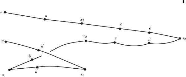
Figure 5: A zipping path $\lambda(x,y)\subset\hat{M}^{2}(f)$. Here $s_{1},s_{2},s_{3}\in\rm{Sing}(f)$ and $(x_{1},x_{2},s_{3})$ stands for a triple point on $M^{3}(f)$ and $(x,y)\in M^{2}(f)$. Similarly, all the pairs like $(a,a^{\prime})$, $(b,b^{\prime})\in\lambda(x,y)$ are in $M^{2}(f)$.

Before we can describe the next more serious result, let us go back to the condition $\Phi(f)=\Psi(f)$ which occurs in Definition 7, and right now we will continue to stick to 3-dimensional representations of $G$. For $f:X^{3}\to\widetilde{M^{3}(G)}$ we have $\rm{Sing}(f)\subset X^{3}$, the mortal singularities, not to be mixed up with the immortal singularities of $\widetilde{M^{3}(G)}$. With this, let

$$\Phi(f)\supset M^{2}(f)\subset X^{3}\times X^{3}\supset\rm{Sing}(f),$$

where the simplified notation $\rm{Sing}(f)$ means $\rm{Diag}(\rm{Sing}(f))$. Let also denote

$$\hat{M}^{2}(f)=M^{2}(f)\cup\rm{Sing}(f).$$

With all these things, the condition $\Psi(f)=\Phi(f)$ can also be expressed as follows: any $(x,y)\in M^{2}(f)$ can be joined, inside $\hat{M}^{2}(f)$, by a continuous path to the singularities. We call such a path a zipping path $\lambda(x,y)\subset\hat{M}^{2}(f)$, or, also, a zipping strategy. Without trying to be more pedantic concerning this definition, Figure 5 should give a clear picture of what a zipping path means.

So retain that the condition $\Phi(f)=\Psi(f)$ means that for every $(x,y)\in M^{2}(f)$ there is a zipping path $\lambda(x,y)$. This is certainly not unique for a given $(x,y)$.

Our $M^{3}(G)$ is a metric space. On the various handles one can define Riemannian metrics compatible on intersections. This lifts then to metrics on $\widetilde{M^{3}(G)},X^{3},X^{3}\times X^{3}$, which are well-defined up to quasi-isometry. With this, we can put up the following

Definition 13.

For $(x,y)\in M^{2}(f)$,

$$l(x,y)=\underset{\lambda}{\rm{inf}}\{\rm{length\ of\ the\ zipping\ path\ }\lambda(x,y)\}.$$

Theorem 4 (Uniform zipping length; V. Poénaru, [57]).

For any finitely presented group $G$, there is a representation $f:X^{3}\to\widetilde{M^{3}(G)}$ which is not only locally compact and equivariant, like in Theorem 3, but also has a uniformly bounded zipping path, i.e. there is a $K>0$ such that for all $(x,y)\in M^{2}(f)$ we have $l(x,y)<K$.

The proof is to be found in [57]. Just like for equivariance, the bounded zipping length has to be forced. The group structure is essential for the proof and we conjecture that for $Wh^{3}$ there is no bounded zipping length. Also, strangely enough, the proof of Theorem 4 requires an infinite process.

3.5 Comments concerning the proofs of Theorems 3 and 4

Concerning the locally finiteness in Theorem 3, in order to achieve it, we have to use the so-called “bi-collared handles” which we will describe a bit more in Part II of this survey.

Topologically speaking, a bi-collared handle is a 3-dimensional handle with the lateral surface removed (or, rather, sent to infinity). There are also two layered structures in this 3-dimensional object, one coming from the attaching zone, the other one going towards that removed lateral surface. With this, when a $(\lambda+1)$-handle is to be attached to the union of all handles of index $\mu\leq\lambda$, then the various intersections $\{$attaching zones of $(\lambda+1)$-handles$\}\cap\{$a given $\mu$-handle$\}$ (and for a given $\mu$-handle there are infinitely many of them), can be corralled towards infinity, insuring thus our local finiteness.

We move now to the equivariant part of Theorem 3, and there we need a symmetry-forcing procedure of which we only present here an abstract version. In [57] this piece of abstract nonsense is transformed into geometry.

So, we are given a simply-connected simplicial complex $X$, endowed with a free action of some discrete group $G$, $G\times X\to X$. We are also given a second simplicial complex $Y$, coming with a non-degenerate simplicial map $F:Y\to X$. Think here of $G\times X\to X$ as being our $G\times\widetilde{M^{3}(G)}\to\widetilde{M^{3}(G)}$ and of $F:Y\to X$ as being some locally-finite representation, not yet equivariant.

If $X^{(\epsilon)}$, $Y^{(\epsilon)}$ are the respective $\epsilon$-skeleta, it is assumed here that the map $F:Y^{(0)}\to X^{(0)}$ is surjective, with countable fibers. For the simplicity of the exposition, we assume $X$ and $Y$ to be 2-dimensional.

Proposition 3.

There is an extension $F_{1}:Z\to X$ of $F:Y\to X$, coming with the commutative diagram

$$\begin{diagram}$$

which is such that:

• The map $F_{1}$ is simplicial and non-degenerate;

• $Z$ is geometrically simply connected;

• There is a free action $G\times Z\to Z$ such that $F_{1}$ is equivariant.

Sketch of proof.

We choose arbitrarily an indexing by the natural integers $\mathbb{Z}_{+}$ of each fiber $F^{-1}(x),\ x\in X^{(0)}$, i.e. we trivialize $Y^{(0)}$ as $Y^{(0)}=X^{(0)}\times\mathbb{Z}_{+}$. We force then an action $G\times Y^{(0)}\to Y^{(0)}$, by $g(x,z_{+})=(gx,z_{+})$.

Next, we construct an intermediary simplicial space $Y\subset Z_{0}\subset Z$ with the following spare parts $Z_{0}^{(0)}=Y^{(0)}$, $Z_{0}^{(\epsilon)}=G\times Y^{(\epsilon)}$, for $\epsilon=1,2$.

We put together these spare parts as follows. Whenever at level $Y$ we have the face-operation $\nu_{i}^{(\epsilon)}:Y^{(\epsilon)}\to Y^{(\epsilon-1)}$, then we force the face relations: $\nu_{i}^{\epsilon}(gs^{\epsilon})=g(\nu_{i}^{\epsilon}s^{\epsilon})$, for $Z_{0}$.

Concretely, this means that, when at level $Y$ we have things like

$$\partial s^{1}=s_{1}^{0}-s_{2}^{1},\ \mbox{ or }\partial s^{2}=s_{0}^{1}-s_{1}^{1}+s_{2}^{1},$$

then at level $Z_{0}$ we have

$$\partial gs^{1}=gs_{1}^{0}-gs_{2}^{1},\mbox{ and }\partial gs^{2}=gs_{0}^{1}-gs_{1}^{1}+gs_{2}^{1},\mbox{for any }g\in G.$$

Moreover, we can define the map $F_{0}:Z_{0}\to Y$ by $F_{0}(gs^{\epsilon})=gF_{0}(s^{\epsilon})$. This map is certainly equivariant but $Z_{0}$ is still not gsc.

So here is how we force this too, continuing to stay equivariant (and the concrete geometric realization of this abstract nonsense story will stay locally-finite too).

Let $T\subset Z_{0}^{(1)}$ be a maximal tree, which misses, exactly, the edges $e_{1},e_{2},\ldots$ of $Z_{0}$. In $Z_{0}^{(1)}$, we chose then a family of closed loops $\lambda_{i}$ with geometric intersection matrix $\lambda_{i}\cdot e_{j}=\delta_{ij}$.

Let $D^{2}_{i}$ be an abstract disk cobounding $\lambda_{i}$. In $Z_{0}$ we have loops $g\lambda_{i}$ for every $i$ and every $g\in G$. With this we construct the space

$$Z\equiv Z_{0}\underset{\sum g\lambda_{i}}{\bigcup}gD^{2}_{i}.$$

Clearly $Z$ is gsc and, with $\pi_{1}X=0$, the equivariant map $F_{1}:Z\to X$ should now be obvious. ∎

All this was purely abstract stuff, and to prove Theorem 3 we need to combine it with the technology of bi-collared handles, making the local-finiteness also achieved. But there is here a bit more to be done.

If we leave things as they are now, we have nasty Cantorian accumulation transversal to the double line, like in the next section. We avoid it by an appropriate “decantorianization”, which we will not describe here. And we need to avoid them for the proof that all groups are qsf.

With this, we have finished with Theorem 3 and we can comment now Theorem 4. Actually, both Theorem 3 and Theorem 4 are important steps in the proof that all groups are qsf, see here Part II of this survey.

Let us say that, when Theorem 3 has been proved, it leaves we with a representation with all the features from the Theorem 3 in question, namely the following:

$\left(1-29\right)$ $$f:X^{3}\to\widetilde{M^{3}(G)}.$$

There is no reason, of course, that for the double points

$\left(1-30\right)$ $$(x,y)\in M^{2}(f)\subset X^{3}\times X^{3},$$

and for their zipping paths, we should have uniformly bounded zipping length. So here is what we do about that.

Staying locally-finite and equivariant, we add now bi-collared handles to (1 – 29), moving to a new representation which extends (1 – 29):

$\left(1-31\right)$ $$f_{1}:X_{1}^{3}\to\widetilde{M^{3}(G)},$$

where, by creating additional zipping paths, we force the double points of (1 – 29), $M^{2}(f)\subset M^{2}(f_{1})\subset X_{1}^{3}\times X_{1}^{3}$, to have uniformly bounded zipping length. The uniform bound is here a simple function of the size of the fundamental domain of the basic action $G\times\widetilde{M^{3}(G)}\to\widetilde{M^{3}(G)}$.

Next, by a second extension, we force the double points in $M^{2}(f_{1})-M^{2}(f)$ to have uniformly bounded zipping length too. But then, also, more uncontrolled double points have been created.

So, we need a full infinite sequence of bigger and bigger representations $f_{n}:X^{3}_{n}\to\widetilde{M^{3}(G)},n=1,2,3\ldots$ coming with the commutative diagram

$$\begin{diagram}$$

and such that for any double point $(x,y)\in M^{2}(f_{n})\subset M^{2}(f_{n+1})$ there is a zipping path of uniformly bounded zipping length in $f_{n+1}:X^{3}_{n+1}\to\widetilde{M^{3}(G)}$, leaving the rest of the double points $M^{2}(f_{n+1})-M^{2}(f_{n})$ completely uncontrolled. That uniform bound is, of course, $n$-dependant. The big issue is to make this infinite process converge, see [57] for details.

And retain also that an infinite process is actually necessary for achieving the desired uniformly bounded zipping length, staying locally-finite and equivariant, at the same time. (Of course some work is necessary for achieving all these things, simultaneously, see [57]).

4 Appendix: a chaotic 2-dimensional REPRESENTATION of the Whitehead manifold

The present section is not concerned with groups nor with group actions, but it should show how wild the accumulation pattern for the double points set of a representation can be. And, in real life, i.e. in geometric group theory, phenomena like those exhibited now, will be avoided, like hell, via the so-called “decantorianization”. [An idea of the process in question is suggested by Figure 2.7.1 in [65], a figure which is directly related to the material that we will present now].

Theorem 5 (V. Poénaru - C. Tanasi, [63]).

There exists a locally-finite, 2-dimensional representation for the Whitehead manifold $Wh^{3}$, call it

$\left(1-32\right)$ $$f:X^{2}\to Wh^{3},$$

with the following features:

• The $X^{2}$ is gotten from a point by infinitely many dilatations. (We say it is “collapsible”, a property stronger than gsc. So $X^{2}$ is certainly gsc too).

• We have $M_{3}(f)=\emptyset$, and each connected component of the $M_{2}(f)$ is a finite tree, based at a mortal singularity.

• There are contact lines $\Lambda\subset X^{2}$ which are tight transversals (a term to be soon explained), to $M_{2}(f)\subset X^{2}$, such that $\Lambda\cap M_{2}(f)$ accumulates on a Cantor set.

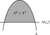
Figure 6: Non-tight transversal.

We shall sketch the proof of this theorem below, but the full proof and explanations concerning its connections to chaos theory are presented in [63]. Here are, to begin with, some comments:

Remark 4.1.

• The fact that the transversal $\Lambda$ is tight means that Figure 6 is forbidden for it.

• The accumulation pattern of $(\Lambda\cap M^{2}(f))$ is governed by a dynamical pattern which is the same as that of a Julia set for a real quadratic polynomial map $f_{\lambda}$ with $\lambda$ outside of the Mandelbrot set (the set of those $\lambda$’s for which $\lambda\in\mbox{ Julia }(f_{\lambda})$), i.e. letting things become complex. And, as it is well-known, for $\lambda$ outside of the Mandelbrot set, Julia$(f_{\lambda})=$ Cantor set.

  We will sketch below this dynamical pattern, without going into its connection with Julia and Mandelbrot, i.e. its connection with chaos. We will just record here that, years ago, it was John Hamal Hubbard who opened the eyes to the second author (V.P.) on the connection between his work on representations and the Julia sets.

  Finally, we believe that there is here a big connection between wild low-dimensional topology and chaos theory, a connection undoubtedly deserving to be explored.

• In a certain sense, the representation (1 – 32) above is the simplest 2-dimensional representation of $Wh^{3}$. Of course, the Whitehead manifold is very far from the highly symmetrical objects $\widetilde{M^{3}(G)}$’s with which the present survey paper deals, and, the kind of chaotic behaviour which (1 – 32) has, is carefully avoided for the representations of $\widetilde{M^{3}(G)}$ (see here Theorem 5 in Part II).

We go now to our Theorem 5 above. For pedagogical-expository reasons, we will not exhibit here the collapsible (1 – 32), but a variant of it

$\left(1-33\right)$ $$f_{1}:K^{2}\to Wh^{3},$$

with a $K^{2}$ which is not collapsible, but only contractible. All the other features of (1 – 32) will be there, nevertheless. It is actually not hard, afterwards, to go from (1 – 33) to the collapsible (1 – 32), by some unglueing of double lines $f_{1}(M^{2}(f_{1}))$; basically, one has to change the Figure 2.6 in [63] to Figure 2.8 in the same paper.

In order to explain the (1 – 33), we start with a modification of the construction from Figure 2 and, for convenience, we will change the notations $D_{1},C_{1},b,c$ from Figure 2 into

$\left(1-34\right)$ $$D_{n},C_{n},b_{n},c_{n}.$$

Here comes now a more serious change. At the level of our Figure 2, the disk $D_{1}$ was glued to itself along $[b,c]$. Now, instead of letting $D_{n}$ be glued to itself along $[b_{n},c_{n}]$, we only let it stay glued along the shorter $[a^{\prime}_{n},a^{\prime\prime}_{n}]$ from Figure 2.5 in [63]. With this, the fat points $a^{\prime}_{n},a^{\prime\prime}_{n}$ become mortal (or undrawable) singularities and the dotted lines in Figure 2.5 of [63] are in $M_{2}(f_{1})$. Also, at the level of $D_{n}$, which from now on is conceived as being self-glued along $[a^{\prime}_{n},a^{\prime\prime}_{n}]$, the line $C_{n}$ is a simple closed loop. With these things our $K^{2}$ is the infinite union of the disks $D_{n}$, namely $K^{2}=D_{1}\cup D_{2}\cup D_{3}\cup\ldots$ where the disks $D_{i}$ are like in Figure 2.4 of [63].

And, with this, comes now the basic identification, or gluing process of $D_{n+1}$ to $D_{n}$:

$\left(1-35\right)$ $$C_{n}\equiv\partial D_{n+1},\forall n.$$

Figure 2.9 in [63] should suggest how the double point set $M_{2}(f_{1})$ starts occurring, when $D_{1}$ and $D_{2}$ interact with $D_{0}$ and then $D_{2}$ with $D_{1}$. Of course, this is only the beginning of an infinite cascade where,

$\left(1-36\right)$ $$\mbox{ for each }n\mbox{ the }D_{n}\mbox{ interacts with }D_{n+1},D_{n+2},\ldots.$$

When one looks at the infinite cascade unleashed in Figure 2.9 from [63], we see double points of $f_{1}$ occurring on each $C_{n}$ and each $\partial D_{n}$, typically represented as a letter, $p$ or $q$, with upper and lower indices. Keep in mind that, because of (1 – 35), the same double point occurs both on $C_{n}$ and on $\partial D_{n+1}$.

For a given double point, we will use the definitions

$\left(1-37\right)$ $$\{\mbox{flavour of the double point}\}\equiv\{\mbox{the number of lower indices}\}+1,\mbox{ and }$$

$$\{\mbox{color of the double point}\}\equiv\{\mbox{the letter }(p\mbox{ or }q),\mbox{ and the unique upper index}\}.$$

The canonical isomorphism $\partial D_{n+1}=C_{n}$ is both color and flavour preserving.

The schematical Figure 7 can help in visualizing what is going on. In this figure, $s_{n}$ stands for the singularities $a_{n}^{\prime}$ or $a_{n}^{\prime\prime}$. Also, the numbers which occur on the lower line are connected with the index of the singularity $s_{n}$ which generates them, and have nothing to do with color or flavour.

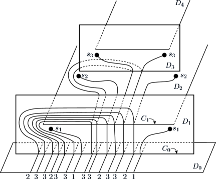
Figure 7: The dynamical algorithm.

We will end this discussion with the explicit description of the dynamical algorithm which generates the set $M_{2}(f_{1})\cap\Lambda$, for a typical tight transversal $\Lambda=C_{n}$.

We start with Figure 2.10 in [63] where, to begin with, we have just the generic fat lines $C,\partial D$. We will explain how the rest of the figure is generated by the Julia dynamical algorithm for generating $M_{2}(f_{1})\cap\Lambda$, and, eventually, the numbers which will start popping up both on $C$ and on $\partial D$, will correspond to the flavours in (1 – 37).

We have the initial points $a_{up}$ and $a_{down}\in C$. Then, starting from them, we draw horizontal dotted lines to $\partial D$, generating the two points $1\in\partial D$. By dynamical self-consistency, we also draw the two $1\in C$, in agreement to the isomorphism $\partial D=C$, which becomes now flavour preserving. From the two points $1\in C$ we generate next four points $2\in\partial D$ and then this process continues indefinitely.

Much more details concerning this story are provided in [63].

References

- [1] I. Agol, The virtual Haken conjecture, Doc. Math., J. DMV 18 (2013), 1045–1087.
- [2] L. Bessières, G. Besson, M. Boileau, S. Maillot and J. Porti. Geometrisation of 3-manifolds. EMS Tracts in Mathematics, volume 13. European Mathematical Society, Zurich, 2010.
- [3] S.G. Brick, Quasi-isometries and ends of groups, J. Pure Appl. Alg. 86 (1993), No. 1, 23–33.
- [4] S.G. Brick, Quasi-isometries and amalgamations of tame combable groups, Inter. J. Alg. Comp. 5 (1995), No. 2, 199–204.
- [5] S.G. Brick and M.L. Mihalik, The QSF property for groups and spaces, Math. Zeit. 220 (1995), No. 2, 207–217.
- [6] J.W. Cannon, Almost convex groups, Geom. Ded. 22 (1987), 197–210.
- [7] J.W. Cannon, W.J. Floyd, M.A. Grayson and W.P Thurston, Solvgroups are not almost convex, Geom. Ded. 31 (1989), No. 3, 291–300.
- [8] M. Coornaert, T. Delzant and A. Papadopoulos. Géométrie et théorie des groupes. Les groupes hyperboliques de Gromov. Lecture Notes in Mathematics, 1441. Berlin etc.: Springer-Verlag. x, 165 p., 1990.
- [9] M.W. Davis, Groups generated by reflections and aspherical manifolds not covered by Euclidian Spaces, Ann. Math. (2) 117 (1983), 293–324.
- [10] M.W. Davis and M. Shapiro Coxeter groups are almost convex, Geom. Ded. 39 (1991), No. 1, 55–57.
- [11] C.H. Edwards, Open 3-manifolds which are simply connected at infinity, Proc. Am. Math. Soc. 14 (1963), 391–395.
- [12] D. Epstein, J.W. Cannon, D. Holt, S. Levy, M. Paterson, and W.P. Thurston. Word processing in groups. Boston, MA etc.: Jones and Bartlett Publishers, 1992.
- [13] M.H. Freedman, The topology of four-dimensional manifolds, J. Diff. Geom. 17 (1982), 357–453.
- [14] M.H. Freedman and F. Quinn. Topology of 4-manifolds. Princeton Mathematical Series, vol. 39, Princeton University Press, Princeton, NJ, 1990.
- [15] L. Funar, On discrete solvgroups and Poénaru condition, Arch. Math. 72 (1999), 81–85.
- [16] L. Funar and S. Gadgil, On the geometric simple connectivity of open manifolds, I.M.R.N. 24 (2004), No. 24, 1193–1248.
- [17] L. Funar and D.E. Otera, On the wgsc and qsf tameness conditions for finitely presented groups, Groups Geom. Dyn. 4 (2010), No. 3, 549–596.
- [18] D. Gabai, Valentin Poénaru’s program for the Poincaré conjecture, in Yau, S.-T. (ed.), “Geometry, topology and physics for Raoul Bott”. Cambridge, MA: International Press. Conf. Proc. Lect. Notes Geom. Topol. 4 (1995), 139–166.
- [19] D. Gabai, The Whitehead manifold is a union of two Euclidean spaces, J. Topol. 4 (2011), No. 3, 529—534.
- [20] S.M. Gersten and J.R. Stallings, Casson’s idea about -manifolds whose universal cover is , Inter. J. Alg. Comp. 1 (1991), No. 4, 395–406.
- [21] E. Ghys and P. de la Harpe (Eds.), Sur les groupes hyperboliques d’après M. Gromov, Progress in Math., vol. 3, Birkhauser, 1990.
- [22] J. Glimm, Two Cartesian products which are Euclidean spaces, Bull. Soc. Math. France 88 (1960), 131–135.
- [23] M. Gromov, Infinite groups as geometric objects. Proc. Int. Congr. Math., Warszawa 1983, Vol. 1 (1984), 385–392.
- [24] M. Gromov, Hyperbolic groups, Essays in Group Theory (S. Gersten Ed.), MSRI publications, n. 8, Springer-Verlag, 1987.
- [25] M. Gromov, Asymptotic invariants of infinite groups, Geometric group theory, Vol. 2 (Sussex, 1991), 1–295, London Math. Soc. Lecture Note Ser. 182, Cambridge Univ. Press, Cambridge, 1993.
- [26] M. Gromov, Random walk in random groups, Geom. Funct. Anal. 13 (2003), No. 1, 73–146.
- [27] L. Guillou and A. Marin (Eds.). A la recherche de la topologie perdue. Progress in Mathematics, Vol. 62, Birkhauser, 1986.
- [28] F. Haglund and D.T. Wise, A combination theorem for special cube complexes, Ann. Math. (2) 176 (2012), No. 3, 1427–1482.
- [29] S. Hermiller and J. Meier, Tame combings, almost convexity and rewriting systems for groups, Math. Zeit. 225 (1997), No. 2, 263–276.
- [30] I. Kapovich, A note on the Poénaru condition, J. Group Theory 5 (2002), No. 1, 119–127.
- [31] D.R. McMillan, Some contractible open 3-manifolds, Trans. Am. Math. Soc. 102 (1962), 373–382.
- [32] M.L. Mihalik and S.T. Tschantz, Tame combings of groups, Tran. Am. Math. Soc. 349 (1997), No. 10, 4251–4264.
- [33] C.F. Miller and M. Shapiro, Solvable Baumslag-Solitar groups are not almost convex, Geom. Ded. 72 (1998), No. 2, 123–127.
- [34] J. Morgan, G. Tian. Ricci flow and the Poincaré conjecture. Clay Mathematics Monographs 3. Providence, RI: American Mathematical Society (AMS); Cambridge, MA: Clay Mathematics Institute. xlii + 521 pp., 2007.
- [35] J. Morgan, G. Tian. The geometrization conjecture. Clay Mathematics Monographs 5. Providence, RI: American Mathematical Society (AMS); Cambridge, MA: Clay Mathematics Institute. ix + 291 pp., 2014.
- [36] R. Myers, Contractible open 3-manifolds which are not covering spaces, Topology 27 (1988), No. 1, 27–35.
- [37] M.H.A. Newman, J.H.C. Whitehead, On the group of a certain linkage, Quart. J. Math. Oxf. Ser. 8 (1937), 14–21.
- [38] D.E. Otera, Topological tameness conditions of spaces and groups: Results and developments, Lith. Math. J. 56 (2016), No. 3, 357–376.
- [39] D.E. Otera and V. Poénaru, “Easy” Representations and the qsf property for groups, Bull. Belgian Math. Soc. - Simon Stevin 19 (2012), No. 3, 385–398.
- [40] D.E. Otera and V. Poénaru, Tame combings and easy groups, Forum Math. 29 (2017), No. 3, 665–680.
- [41] D.E. Otera and V. Poénaru, Finitely presented groups and the Whitehead nightmare, Groups Geom. Dyn. 11 (2017), No. 1, 291–310.
- [42] D.E. Otera, V. Poénaru and C. Tanasi, On Geometric Simple Connectivity, Bulletin Mathématique de la Société des Sciences Mathématiques de Roumanie. Nouvelle Série, Tome 53 (101) (2010), No. 2, 157–176.
- [43] D.E. Otera and F.G. Russo, On the wgsc property in some classes of groups, Mediterr. J. Math. 6 (2009), No. 4, 501–508.
- [44] D.E Otera, F.G. Russo and C. Tanasi, On 3-dimensional wgsc inverse-representations of groups, Acta Math. Hung. 151 (2017), No. 2, 379–390.
- [45] C.D. Papakyriakopoulos, On Dehn’s lemma and the asphericity of knots, Ann. Math. (2) 66 (1957), 1–26.
- [46] G. Perelman, The entropy formula for the Ricci flow and its geometric applications, ArXiv: math/0211.159 [math.DG] (2002).
- [47] G. Perelman, Ricci flow with surgery on three-manifolds, ArXiv: math/0303.109 [math.DG] (2003).
- [48] G. Perelman, Finite extinction time for the solutions of the Ricci flow on certain three-manifolds, ArXiv: math/0307.245 [math.DG] (2003).
- [49] V. Poénaru, On the equivalence relation forced by the singularities of a non-degenerate simplicial map, Duke Math. J. 63 (1991), No. 2, 421–429.
- [50] V. Poénaru, Killing handles of index one stably and , Duke Math. J. 63 (1991), No. 2, 431–447.
- [51] V. Poénaru, Almost convex groups, Lipschitz combing, and for universal covering spaces of closed -manifolds, J. Diff. Geom. 35 (1992), No. 1, 103–130.
- [52] V. Poénaru, The collapsible pseudo-spine representation theorem, Topology 31 (1992), No. 3, 625–656.
- [53] V. Poénaru, Geometry “à la Gromov” for the fundamental group of a closed -manifold and the simple connectivity at infinity of , Topology 33 (1994), No. 1, 181–196.
- [54] V. Poénaru, and simple homotopy type in dimension 3, Contemporary Math. AMS, 239 (1999), 1–28.
- [55] V. Poénaru, On the 3-Dimensional Poincaré Conjecture and the 4-Dimensional Smooth Schoenflies Problem, arXiv: math/0612554 [math.GT], 2006.
- [56] V. Poénaru, Discrete symmetry with compact fundamental domain, and geometric simple connectivity - A provisional Outline of work in Progress, arXiv: 0711.3579 [math.GT].
- [57] V. Poénaru, Equivariant, locally finite inverse representations with uniformily bounded zipping length, for arbitrary finitely presented groups, Geom. Ded. 167 (2013), 91–121.
- [58] V. Poénaru, Geometric simple connectivity and finitely presented groups, arXiv: 1404.4283 [math.GT].
- [59] V. Poénaru, All finitely presented groups are qsf, arXiv: 1409.7325 [math.GT].
- [60] V. Poénaru, Geometric simple connectivity and low-dimensional topology, Geometric topology and set theory. Collected papers. Dedicated to the 100th birthday of Professor Lyudmila Vsevolodovna Keldysh. Transl. from the Russian. Moscow: Maik Nauka/Interperiodica. Proceedings of the Steklov Institute of Mathematics 247, 195–208 (2004) and Tr. Mat. Inst. Steklova 247, 214–227 (2004).
- [61] V. Poénaru, A glimpse into the problems of the fourth dimension, Proceedings of the conference “Geometry in History”, to appear.
- [62] V. Poénaru and C. Tanasi, -weakly almost convex groups and , Geom. Ded. 48 (1993), No. 1, 57–81.
- [63] V. Poénaru and C. Tanasi, Representatioin of the Whitehead manifold and Julia sets, Ann. Fac. Sci. Toulouse, Sér. 6 4 (1995), No. 3, 665–694.
- [64] V. Poénaru and C. Tanasi, Some remarks on geometric simple connectivity, Acta Math. Hung. 81 (1998), No. 1-2, 1–12.
- [65] V. Poénaru and C. Tanasi, Equivariant, Almost-Arborescent representations of open simply-connected 3-manifolds; A finiteness result, Mem. AMS, 800, 88 pp., 2004.
- [66] V. Poénaru and C. Tanasi, A group-theoretical finiteness theorem, Geom. Ded. 137 (2008), No. 1, 1–25.
- [67] A. Shapiro and J.H.C. Whitehead, A proof and extension of Dehn’s lemma, Bull. Am. Math. Soc. 64 (1958), 174–178.
- [68] M. Shapiro and M. Stein, Almost convex groups and the eight geometries, Geom. Ded. 55 (1995), No. 2, 125–140.
- [69] L.C. Siebenmann, On detecting Euclidean space homotopically among topological manifolds, Invent. Math., 6 (1968), 263–268.
- [70] J.R. Stallings, The piecewise linear structure of the Euclidean space, Proc. Camb. Math. Philos. Soc. 58 (1962), 481–488.
- [71] J.R. Stallings, On torsion-free groups with infinitely many ends, Ann. Math. (2) 88 (1968), 312–334.
- [72] J.R. Stallings. Group theory and three-dimensional manifolds. Yale Mathematical Monographs. 4. New Haven-London: Yale University Press, 1971.
- [73] J.R. Stallings, Brick’s quasi-simple filtrations for groups and -manifolds, Geometric group theory, Vol. 1 (Sussex, 1991), 188–203, London Math. Soc. Lecture Note Ser., 181, Cambridge Univ. Press, Cambridge, 1993.
- [74] D. Sullivan and W.P. Thurston, Manifolds with canonical coordinate charts: Some examples, Enseign. Math. II. Sér. 29 (1983), 15–25.
- [75] C. Tanasi, Sui gruppi semplicemente connessi all’infinito, Rend. Ist. Mat. Univ. Trieste 31 (1999), No. 1-2, 61–78.
- [76] C. Thiel, Zur fast-Konvexitat einiger nilpotenter Gruppen, Universitat Bonn Mathematisches Institut, Bonn (1992) Dissertation, Rheinische Friedrich-Wilhelms-Universitat Bonn, Bonn, 1991
- [77] W.P. Thurston. Three-dimensional geometry and topology. Vol. 1. Princeton Mathematical Series, 35. Princeton University Press, Princeton, NJ, 1997.
- [78] T.W. Tucker, Non-compact -manifolds and the missing boundary problem, Topology 73 (1974), 267–273.
- [79] C.T.C. Wall, Open 3-manifolds which are 1-connected at infinity, Quart. J. Math. Oxf. Ser. (2) (1965), No. 16, 263–268.
- [80] C.T.C. Wall, Geometrical connectivity. I, II, J. Lond. Math. Soc. (2) 3 (1971), 597–604; 605–608.
- [81] J.H.C. Whitehead, A certain open manifold whose group is unity, Quart. J. Math. Oxf. Ser. 6 (1935), 268–279.
- [82] D.G. Wright, Contractible open manifolds which are not covering spaces, Topology 31 (1992), No. 2, 281–291.