Chemical Diversity in Three Massive Young Stellar Objects associated with 6.7 GHz CH₃OH Masers

Abstract

We have carried out observations in the 42$-$46 and 82$-$103 GHz bands with the Nobeyama 45-m radio telescope, and in the 338.2$-$339.2 and 348.45$-$349.45 GHz bands with the ASTE 10-m telescope toward three high-mass star-forming regions containing massive young stellar objects (MYSOs), G12.89+0.49, G16.86$-$2.16, and G28.28$-$0.36. We have detected HC₃N including its ¹³C and D isotopologues, CH₃OH, CH₃CCH, and several complex organic molecules (COMs). Combining our previous results of HC₅N in these sources, we compare the $N$(HC₅N)/$N$(CH₃OH) ratios in the three observed sources. The ratio in G28.28$-$0.36 is derived to be $0.091^{+0.109}_{-0.039}$, which is higher than that in G12.89+0.49 by one order of magnitude, and that in G16.86$-$2.16 by a factor of $\sim 5$. We investigate the relationship between the $N$(HC₅N)/$N$(CH₃OH) ratio and the $N$(CH₃CCH)/$N$(CH₃OH) ratio. The relationships of the two column density ratios in G28.28$-$0.36 and G16.86$-$2.16 are similar to each other, while HC₅N is less abundant when compared to CH₃CCH in G12.89+0.49. These results imply a chemical diversity in the lukewarm ($T\sim 20-30$ K) envelope around MYSOs. Besides, several spectral lines from complex organic molecules, including very-high-excitation energy lines, have been detected toward G12.89+0.49, while the line density is significantly low in G28.28$-$0.36. These results suggest that organic-poor MYSOs are surrounded by a carbon-chain-rich lukewarm envelope (G28.28$-$0.36), while organic-rich MYSOs, namely hot cores, are surrounded by a CH₃OH-rich lukewarm envelope (G12.89+0.49 and G16.86$-$2.16).

1 Introduction

Molecules are a unique and powerful tool in astronomy. They provide an excellent diagnosis of the physical conditions and processes in the regions where they reside. Progress in this field called astrochemistry is mainly driven by observations from various single-dish and interferometers at millimeter/sub-millimeter wavelengths along with space telescopes at mid- and far-infrared wavelengths (e.g., van Dishoeck, 2017).

Unsaturated carbon-chain molecules tend to be abundant in young low-mass starless cores and deficient in low-mass star-forming cores (Suzuki et al., 1992; Hirota et al., 2009), because they are mainly formed from ionized carbon (C⁺) and atomic carbon (C) via ion-molecule reactions in the early stage of molecular clouds and destroyed mainly by reaction with oxygen atoms and depleted onto dust grains in the late stage. Carbon-chain molecules have been found to be abundant around two low-mass protostars; IRAS 04368+2557 in L1527 (Sakai et al., 2008) and IRAS 15398$-$3359 in Lupus (Sakai et al., 2009a). In these protostars, carbon-chain molecules are newly formed from CH₄ evaporated from dust grains in the lukewarm ($T\sim 20-30$ K) gas (Sakai et al., 2008). Such a carbon-chain chemistry around the low-mass protostars was named warm carbon chain chemistry (WCCC, Sakai et al., 2008). The difference between hot corino chemistry and WCCC is considered to be brought by the different timescale of the starless core phase; the long and short starless core phases lead to hot corino and WCCC sources, respectively (Sakai et al., 2008). Recently, sources possessing both hot corino and WCCC characteristics have been found and high-spatial-resolution observations showed that the spatial distributions of carbon-chain molecules and COMs are different with each other (e.g., Imai et al., 2016).

Saturated complex organic molecules (COMs), organic species consisting of more than six atoms and being rich in hydrogen (Herbst & van Dishoeck, 2009), are classically known to be abundant in the dense and hot ($n>10^{6}$ cm^-3, $T\geq 100$ K) gas around young stellar objects (YSOs). Besides, COMs also have been found in the gas phase before ice thermally evaporates at temperatures above 100 K (Vastel et al., 2014). At these low temperatures, COMs can be desorbed from icy grain mantles via different types of non-thermal desorption process such as: (1) the cosmic-ray desorption mechanism (Reboussin et al., 2014), (2) the chemical desorption mechanism (desorption due to the exothermicity of surface reactions; Garrod et al., 2007), and (3) the photo-desorption (Ruaud et al., 2016). Role of barrier-less gas phase reactions to form COMs was also proposed recently by Balucani et al. (2015). Recent observations show the presence of some COMs, methylformate (HCOOCH₃), dimethyl ether (CH₃OCH₃), and methyl cyanide (CH₃CN), and the complex radical methoxy (CH₃O) in regions where the dust temperature is less than 30 K; pre-stellar cores (Bacmann et al., 2012; Vastel et al., 2014; Potapov et al., 2016) and cold envelopes of low-mass protostars (Öberg et al., 2010; Cernicharo et al., 2012; Jaber et al., 2014). Grain-surface chemistry certainly plays a role, for example in forming hydrogenated species during the prestellar phase (Tielens & Hagen, 1982; Caselli & Ceccarelli, 2012), but not necessarily in the formation of all COMs.

Not only in the low-mass star-forming regions, new questions arise in the chemistry around massive young stellar objects (MYSOs). Fayolle et al. (2015) compared the chemistry between organic-poor MYSOs and organic-rich MYSOs, namely hot cores. They suggested that hot cores are not required to form COMs and temperature and initial ice composition possibly affect complex organic distributions around MYSOs. Green et al. (2014) detected HC₅N, the second shortest cyanopolyynes (HC_2n+1N, $n=1,2,3,...$), in 35 hot cores associated with the 6.7 GHz methanol masers, which give us the exact positions of MYSOs (Urquhart et al., 2013). However, there remained the possibility that the emission of HC₅N comes from the outer cold molecular clouds or other molecular clouds in the large single-dish beam ($\sim 0.95$′). Taniguchi et al. (2017b) carried out observations toward four MYSOs where Green et al. (2014) detected HC₅N, using the Green Bank 100-m telescope (GBT) and the Nobeyama 45-m radio telescope. The four target sources were selected adding three criteria mentioned in Section 2 and we chose three sources showing the highest HC₅N peak intensities (G12.89+0.49, G16.86$-$2.16, and G28.28$-$0.36) and a source showing the low HC₅N peak intensity with the high CH₃CN peak intensities (G10.30$-$0.15). They detected the high-excitation-energy ($E_{\rm{u}}/k\sim 100$ K) lines of HC₅N, which cannot be detected if HC₅N exists in the cold dark clouds, in the three sources (G12.89+0.49, G16.86$-$2.16, and G28.28$-$0.36) and confirmed that HC₅N exists in the warm gas around MYSOs. Therefore, carbon-chain molecules seem to be formed in the lukewarm gas around MYSOs, as well as WCCC sources in the low-mass star-forming regions. At the present stage, we do not know the relationships between carbon-chain molecules and COMs around MYSOs.

In this paper, we report the observational results in the 42$-$46, 82$-$103, 338.2$-$339.2 and 348.45$-$349.45 GHz bands obtained with the Nobeyama 45-m radio telescope and the Atacama Submillimeter Telescope Experiment (ASTE) 10-m telescope toward three MYSOs, G12.89+0.49, G16.86$-$2.16, and G28.28$-$0.36. We derive the rotational temperatures and beam-averaged column densities of HC₃N, CH₃OH, and CH₃CCH (Section 4). We compare the spectra and the chemical composition among the three sources, combining with previous HC₅N data (Taniguchi et al., 2017b), in order to investigate the relationship between carbon-chain species and COMs in high-mass star-forming regions (Section 5).

2 Observations

The observations presented in this paper were conducted in the Nobeyama 45-m radio telescope and the ASTE joint observation program (Proposal ID: JO161001, PI: Kotomi Taniguchi, 2016-2017 season). The observing parameters of each frequency band are summarized in Table 1. The Nobeyama 45-m telescope data have been partly published in Taniguchi et al. (2017b).

The source selection criteria were described in Taniguchi et al. (2017b) as follows:

1. The source declination is above $-21$°,

2. the distance ($D$) is within 3 kpc, and

3. CH₃CN was detected ($\int T_{\rm{mb}}dv>0.5$ K km s^-1 for $J_{K}=5_{0}-4_{0}$ line, Purcell et al., 2006).

Eight sources in the HC₅N-detected source list of Green et al. (2014) meet the above three criteria. We chose three sources among the eight selected sources which show the highest peak intensities of HC₅N ($T_{\rm{mb}}>120$ mK). Table 2 summarizes the properties of our three target sources. The observed positions correspond to the 6.7 GHz methanol maser positions, which show exact positions of the MYSOs (Urquhart et al., 2013).

Table 1: Observing parameters

Frequency	Telescope	Beam size	$\eta_{\rm{mb}}$	$T_{\rm{sys}}$	$\Delta\nu$	$T_{\rm{rms}}$
(GHz)		(′′)	(%)	(K)	(kHz)	(mK)
42$-$46	Nobeyama	37	71	120$-$150	122.07	6$-$14
82$-$103	Nobeyama	18	54	120$-$200	244.14	3$-$6
338$-$349.4	ASTE	22	60	300$-$700	1000	16$-$24

Table 2: Properties of our target sources

Source	R.A.	Decl.	$D$	$V_{\rm{LSR}}$	Other Association
	(J2000)	(J2000)	(kpc)	(km s-1)	UCH II	outflow
G12.89+0.49	18h11m51$\fs$4	-17°31′30″	2.50	33.3	N	Y
G16.86$-$2.16	18h29m24$\fs$4	-15°16′04″	1.67	17.8	N	Y
G28.28$-$0.36	18h44m13$\fs$3	-04°18′03″	3.0	48.9	Y	Y

2.1 Observations with the Nobeyama 45-m Radio Telescope

We carried out observations with the Nobeyama 45-m radio telescope from 2017 January to March. We employed the position-switching mode. The integration time was 20 seconds per on-source and off-source positions. The on-source positions are summarized in Table 2 and the off-source positions were set to be $+15\arcmin$ away in declination. The total integration time is $\sim 1$ hr and 2$-$4.5 hr in the 42$-$46 GHz and 82$-$103 GHz band observations, respectively.

The Z45 receiver (Nakamura et al., 2015) and the TZ receiver (Nakajima et al., 2013) were used in the observations at 42$-$46 GHz and 82$-$103 GHz, respectively. The main beam efficiency ($\eta_{\rm{mb}}$) and the beam size (HPBW) at 43GHz were 71% and $37\arcsec$, respectively. The main beam efficiency and the beam size at 86 GHz were 54% and $18\arcsec$, respectively. The system temperatures were 120$-$150 K and 120$-$200 K during the observations at 42$-$46 GHz and 82$-$103 GHz, respectively. We used the SAM45 FX-type digital correlator (Kamazaki et al., 2012) in frequency settings whose bandwidths and resolutions are 500 MHz and 122.07 kHz for the Z45 observations, and 1000 MHz and 244.14 kHz for the TZ observations, respectively. The frequency resolutions correspond to the velocity resolution of $\sim 0.85$ km s^-1.

The telescope pointing was checked every 1.5 hr by observing the SiO maser line ($J=1-0$; 43.12203 GHz) from OH39.7+1.5 at ($\alpha_{2000}$, $\delta_{2000}$) = (18^h56^m03$\fs$88, +06°38′49$\farcs$8). We used the Z45 receiver for the pointing check during the 42$-$46 GHz band observations and the H40 receiver for the pointing check during the 82$-$103 GHz band observations. The pointing error was less than $3\arcsec$.

The rms noises are 6$-$14 and 3$-$6 mK in $T_{\rm{A}}^{*}$ scale in the 42$-$46 GHz and 82$-$103 GHz bands, respectively. The baseline was fitted with a linear function. The absolute flux calibration error is approximately 10%.

2.2 Observations with the ASTE 10-m Telescope

The observations with the ASTE 10-m telescope were conducted in 2016 September and October. The DASH345 receiver and the WHSF FX-type digital spectrometer (Iguchi & Okuda, 2008; Okuda & Iguchi, 2008) were used. The observed frequency ranges are 338.2$-$339.2 and 348.45$-$349.45 GHz. The main beam efficiency and beam size were 60% and $22\arcsec$, respectively. The system temperatures were between 300 and 700 K, depending on the elevation and weather conditions. The frequency setting was 2048 MHz bandwidth and 1 MHz frequency resolution. The frequency resolution corresponds to 0.86 km s^-1, which is almost equal to that of observations with the Nobeyama 45-m telescope. The total integration time is approximately 1– 2.5 hr, which is different among sources.

We checked the telescope pointing every 2 hr by observing the ¹²CO ($J=3-2$) line from W Aql at ($\alpha_{2000}$, $\delta_{2000}$) = (19^h15^m23$\fs$35, -07°02′50$\farcs$3). The pointing error was less than $2\arcsec$.

The rms noise levels in the line-free regions are 23$-$24, 19$-$20, and 16$-$17 mK in $T_{\rm{A}}^{*}$ scale in G12.89+0.49, G16.86$-$2.16, and G28.28$-$0.36, respectively. Some scans were excluded due to bad baselines. A linear fit was applied for baseline subtraction. The absolute flux calibration error is approximately 10%.

3 Results

We conducted data reduction using the Java Newstar software, an astronomical data analyzing system of the Nobeyama 45-m telescope and the ASTE 10-m telescope.

3.1 Observational Results with the Nobeyama 45-m Radio Telescope

Figure 1 shows the spectra of the main isotopologue HC₃N and its ¹³C and D isotopologues in the three sources obtained with the Nobeyama 45-m radio telescope. We fitted the spectra with a Gaussian function and obtained the spectral line parameters as summarized in Table 3. Two rotational transitions, $J=5-4$ and $10-9$, of the main isotopologue are in the observed frequency bands, and they were detected from all of the three sources. Its three ¹³C isotopologues have been detected from G28.28$-$0.36 with a signal-to-noise (S/N) ratio above 4. HC¹³CCN was not detected in G12.89+0.49, whereas H¹³CCCN was not detected in G16.86$-$2.16. DC₃N was detected in G28.28$-$0.36 with a S/N ratio of 3 and in G16.86$-$2.16 with a S/N ratio above 4. The $V_{\rm{LSR}}$ values agree with the systemic velocities of each source (Table 2).

The line profiles of the main isotopologue show wing emission, suggesting that HC₃N also exists in the molecular outflow (e.g., Shimajiri et al., 2015; Taniguchi et al., 2018). Such wing emission is most prominent in G16.86$-$2.16, where the blue and red components are clearly detected. The red and blue components are prominent in G12.89+0.49 and G28.28$-$0.36, respectively. These features of wing emission of HC₃N are similar to those of CH₃OH (Figure 3), as mentioned later. Hence, the origin of molecular outflows is plausible.

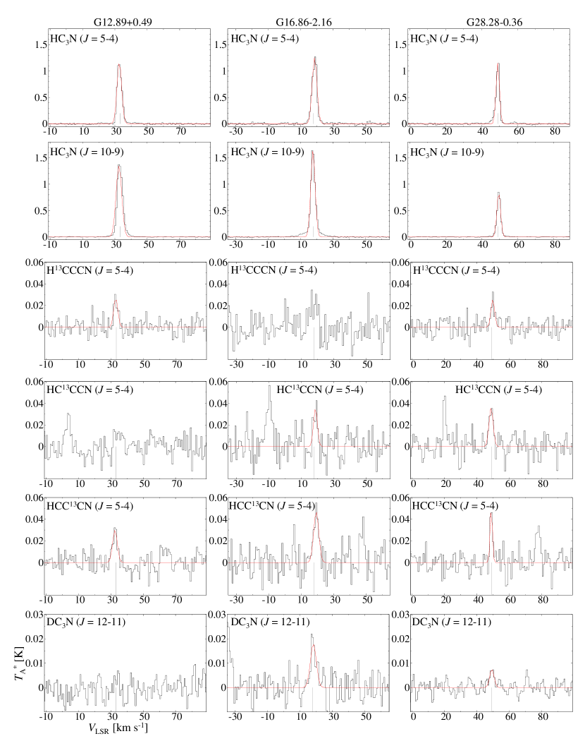
Figure 1: Spectra of the main isotopologue HC₃N and its ¹³C and D isotopologues in the three sources. The red lines show the Gaussian fitting results and gray vertical lines show the systemic velocity for each source.

Table 3: Spectral line parameters of the main isotopologue HC₃N and its ¹³C and D isotopologues in the three sources with the Nobeyama 45-m telescope

			G12.89+0.49					G16.86$-$2.16					G28.28$-$0.36
Species	Frequency	$E_{\rm{u}}/k$	$T_{\rm{mb}}$	FWHM	$\int T_{\mathrm{mb}}dv$	$V_{\rm{LSR}}$		$T_{\rm{mb}}$	FWHM	$\int T_{\mathrm{mb}}dv$	$V_{\rm{LSR}}$		$T_{\rm{mb}}$	FWHM	$\int T_{\mathrm{mb}}dv$	$V_{\rm{LSR}}$
Transition	(GHz)	(K)	(K)	(km s-1)	(K km s-1)	(km s-1)		(K)	(km s-1)	(K km s-1)	(km s-1)		(K)	(km s-1)	(K km s-1)	(km s-1)
HC3N
$J=5-4$	45.490314	6.5	1.64 (4)	3.35 (9)	5.8 (2)	32.8		1.76 (5)	3.50 (12)	6.6 (3)	18.7		1.62 (6)	2.22 (10)	3.8 (2)	49.0
$J=10-9$	90.979023	24.0	2.58 (12)	4.1 (2)	11.3 (8)	32.5		3.15 (7)	3.22 (8)	10.8 (4)	17.7		1.64 (3)	2.39 (5)	4.16 (11)	49.5
H13CCCN
$J=5-4$	44.084172	6.4	0.037 (7)	3.0 (7)	0.12 (4)	33.0		$<0.036$	…	…	…		0.036 (6)	2.7 (5)	0.10 (3)	49.8
HC13CCN
$J=5-4$	45.2973345	6.5	$<0.027$	…	…	…		0.050 (12)	2.8 (8)	0.15 (6)	18.9		0.051 (8)	3.0 (6)	0.16 (4)	48.7
HCC13CN
$J=5-4$	45.3017069	6.5	0.042 (7)	3.4 (7)	0.15 (4)	32.5		0.090 (13)	3.7 (6)	0.36 (8)	19.3		0.073 (13)	1.7 (4)	0.13 (4)	48.8
DC3N
$J=12-11$	101.314818	31.6	$<0.013$	…	…	…		0.034 (6)	4.3 (9)	0.16 (4)	18.2		0.014 (3)	3.2 (7)	0.049 (13)	49.2

Note. — Numbers in the parentheses are the standard deviation of the Gaussian fit, expressed in units of the last significant digits. For example, 1.64 (4) means $1.64\pm 0.04$. The upper limits correspond to the $3\sigma$ limits.

Figure 2 shows the spectra of CH₃CCH obtained with the Nobeyama 45-m radio telescope. Its $J=5-4$ and $6-5$ $K$-ladder lines ($K=0-0$, $1-1$, $2-2$, and $3-3$) were detected from the three sources with a S/N ratio above 4. We fitted the spectra with four-component Gaussian profiles. We fixed the centroid velocities to be the systemic velocities for each source (Table 2). The spectral line parameters are summarized in Table 4. There is no presence of wing emission in the CH₃CCH spectra and the lines are well fitted with the Gaussian profile.

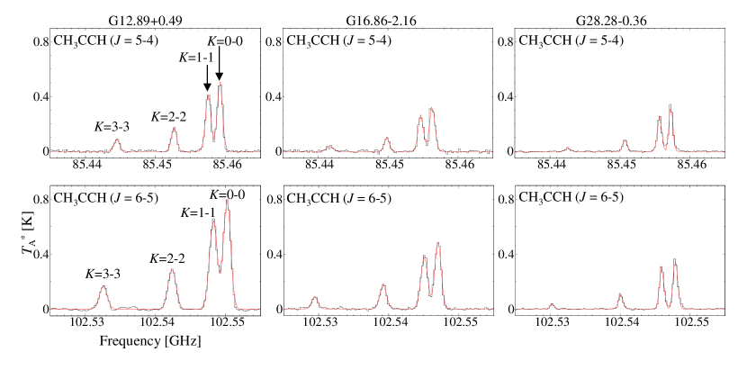
Figure 2: Spectra of CH₃CCH in the three sources. The red lines show the Gaussian fitting results.

Table 4: Spectral line parameters of CH₃CCH in the three sources with the Nobeyama 45-m telescope

			G12.89+0.49				G16.86$-$2.16				G28.28$-$0.36
Transition	Frequency	$E_{\rm{u}}/k$	$T_{\rm{mb}}$	FWHM	$\int T_{\mathrm{mb}}dv$		$T_{\rm{mb}}$	FWHM	$\int T_{\mathrm{mb}}dv$		$T_{\rm{mb}}$	FWHM	$\int T_{\mathrm{mb}}dv$
	(GHz)	(K)	(K)	(km s-1)	(K km s-1)		(K)	(km s-1)	(K km s-1)		(K)	(km s-1)	(K km s-1)
$J=5-4$
$K=0-0$	85.4573003	12.3	0.958 (14)	3.03 (5)	3.09 (6)		0.616 (18)	3.18 (9)	2.08 (8)		0.638 (14)	2.19 (5)	1.49 (4)
$K=1-1$	85.4556667	19.5	0.785 (14)	3.20 (6)	2.67 (7)		0.496 (18)	3.02 (11)	1.59 (8)		0.477 (13)	2.46 (7)	1.25 (5)
$K=2-2$	85.4507663	41.2	0.324 (14)	3.08 (13)	1.06 (6)		0.190 (19)	2.8 (3)	0.57 (8)		0.160 (13)	2.44 (19)	0.42 (5)
$K=3-3$	85.4426012	77.3	0.168 (14)	3.2 (3)	0.56 (7)		0.065 (16)	3.9 (9)	0.27 (9)		0.044 (13)	2.6 (7)	0.12 (5)
$J=6-5$
$K=0-0$	102.5479844	17.2	1.741 (13)	3.51 (3)	6.50 (8)		1.079 (14)	3.07 (5)	3.53 (7)		0.791 (12)	2.16 (4)	1.82 (4)
$K=1-1$	102.5460242	24.5	1.412 (13)	3.81 (4)	5.72 (8)		0.845 (13)	3.26 (6)	2.93 (7)		0.676 (12)	2.09 (4)	1.50 (4)
$K=2-2$	102.5401446	46.1	0.637 (13)	3.75 (9)	2.54 (8)		0.385 (13)	3.19 (13)	1.31 (7)		0.239 (12)	2.09 (12)	0.53 (4)
$K=3-3$	102.5303476	82.3	0.374 (13)	3.61 (14)	1.44 (8)		0.192 (14)	3.0 (2)	0.61 (7)		0.086 (13)	1.8 (3)	0.16 (4)

Note. — Numbers in the parentheses are the standard deviation of the Gaussian fit, expressed in units of the last significant digits.

Nine thermal CH₃OH lines were detected from G12.89+0.49, and eight lines, except for $6_{-2,5}-7_{-1,7}$ $E$ transition, were detected from the other two sources with a S/N ratio above 4 as shown in Figure 3. We fitted the spectra with Gaussian profiles and the spectral line parameters are summarized in Table 5. For the four lines shown in the top panels of Figure 3, we applied the four-component Gaussian fitting. In the same way as for CH₃CCH, the centroid velocities were fixed to be the systemic velocities of each source (Table 2). The wing emission for red and blue velocity components are seen in G16.86$-$2.16, while only the red component is found in G12.89+0.49. In G28.28$-$0.36, no wing emission is seen, which may be due to their lower line intensities.

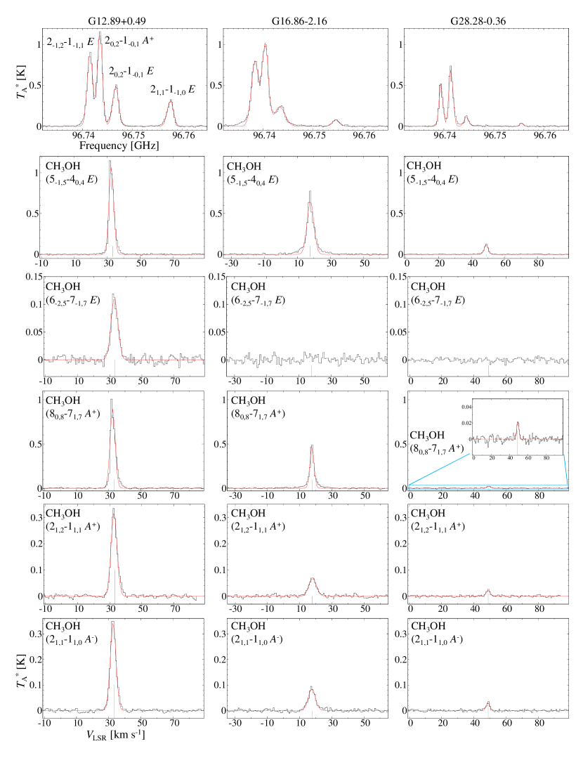
Figure 3: Spectra of CH₃OH in the three sources. The red lines show the Gaussian fitting results and gray vertical lines show the systemic velocity for each source.

Table 5: Spectral line parameters of CH₃OH in the three sources with the Nobeyama 45-m telescope

			G12.89+0.49					G16.86$-$2.16					G28.28$-$0.36
Transition	Frequency	$E_{\rm{u}}/k$	$T_{\rm{mb}}$	FWHM	$\int T_{\mathrm{mb}}dv$	$V_{\rm{LSR}}$		$T_{\rm{mb}}$	FWHM	$\int T_{\mathrm{mb}}dv$	$V_{\rm{LSR}}$		$T_{\rm{mb}}$	FWHM	$\int T_{\mathrm{mb}}dv$	$V_{\rm{LSR}}$
	(GHz)	(K)	(K)	(km s-1)	(K km s-1)	(km s-1)		(K)	(km s-1)	(K km s-1)	(km s-1)		(K)	(km s-1)	(K km s-1)	(km s-1)
$5_{-1,5}-4_{0,4}$ $E$	84.521169	40.4	1.97 (8)	3.44 (14)	7.2 (4)	32.5		1.20 (6)	4.9 (2)	6.2 (4)	17.9		0.222 (8)	2.79 (10)	0.66 (3)	48.9
$6_{-2,5}-7_{-1,7}$ $E$	85.568084	74.7	0.206 (7)	5.06 (17)	1.11 (5)	32.9		$<0.018$	…	…	…		$<0.011$	…	…	…
$8_{0,8}-7_{1,7}$ $A^{+}$	95.169463	83.5	1.82 (7)	3.70 (15)	7.2 (4)	32.4		0.96 (4)	2.92 (13)	2.99 (18)	17.7		0.045 (4)	3.0 (3)	0.14 (2)	49.3
$2_{1,2}-1_{1,1}$ $A^{+}$	95.914309	21.4	0.664 (13)	4.39 (10)	3.10 (9)	32.7		0.141 (4)	5.55 (19)	0.83 (4)	18.0		0.050 (4)	2.8 (3)	0.149 (19)	48.9
$2_{-1,2}-1_{-1,1}$ $E$	96.739362	12.5	1.81 (2)	4.09 (6)	7.87 (15)	$-$		1.63 (2)	5.31 (9)	9.2 (2)	$-$		1.06 (3)	2.80 (10)	3.16 (14)	$-$
$2_{0,2}-1_{0,1}$ $A^{+}$	96.741375	7.0	2.39 (2)	3.60 (4)	9.14 (14)	$-$		2.05 (2)	4.50 (7)	9.81 (19)	$-$		1.42 (3)	3.02 (7)	4.57 (15)	$-$
$2_{0,2}-1_{0,1}$ $E$	96.744550	20.1	0.99 (2)	4.40 (11)	4.66 (15)	$-$		0.485 (18)	7.8 (4)	4.0 (2)	$-$		0.23 (3)	3.5 (5)	0.87 (16)	$-$
$2_{1,1}-1_{1,0}$ $E$	96.755511	28.0	0.64 (2)	4.47 (17)	3.06 (15)	$-$		0.16 (2)	5.2 (8)	0.87 (18)	$-$		0.08 (3)	2.6 (12)	0.22 (14)	$-$
$2_{1,1}-1_{1,0}$ $A^{-}$	97.582804	21.6	0.702 (12)	4.18 (8)	3.12 (8)	32.7		0.172 (7)	5.3 (2)	0.97 (6)	17.6		0.065 (6)	2.7 (3)	0.18 (2)	48.8

Note. — Numbers in the parentheses are the standard deviation of the Gaussian fit, expressed in units of the last significant digits. The upper limits correspond to the $3\sigma$ limits.

Figures 4 and 5 show the spectra in the frequency bands covered with the TZ receiver. Several lines from COMs have been detected with a S/N ratio above 4. An analysis of the COMs requires the simultaneous fitting of multiple species to avoid blending effects with other lines. In our case, detected COMs have similar excitation-energy and such fitting cannot degenerate excitation temperatures and column densities. Therefore, we cannot derive their rotational temperatures and column densities accurately and we will not discuss COMs in the rest of this paper. We summarize the detection and non-detection of COMs in each source in Table 6. G12.89+0.49 is the most line-rich source with strong peak intensities, and both nitrogen-bearing COMs and oxygen-bearing COMs have been detected. On the other hand, only CH₃OH and CH₃CHO were detected with weak peak intensities in G28.28$-$0.36.

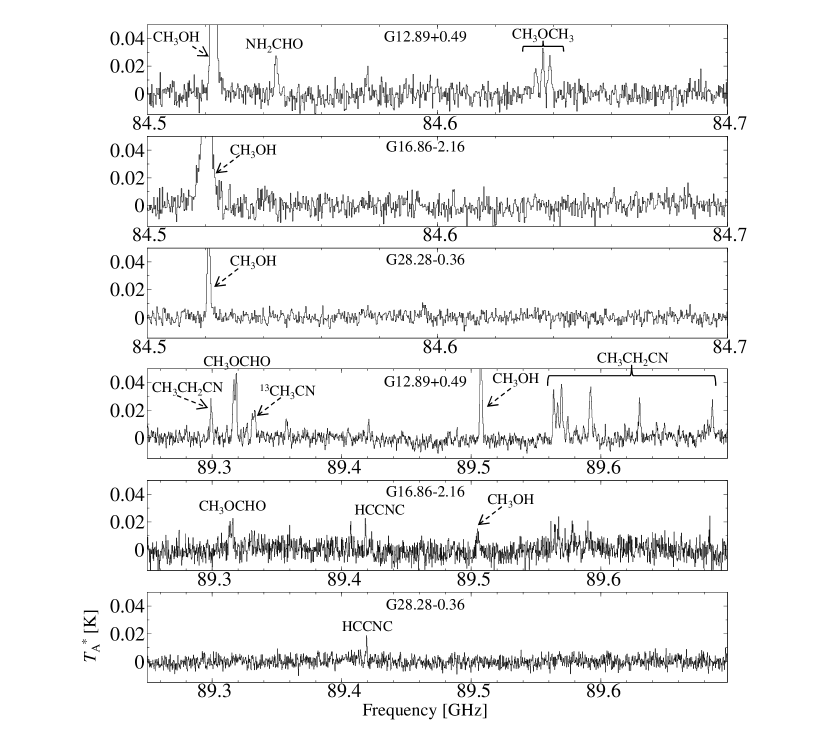
Figure 4: Spectra of the complex organic molecules in the 84.5$-$84.7 and 89.3$-$89.7 GHz bands in the three sources obtained with the Nobeyama 45-m telescope.

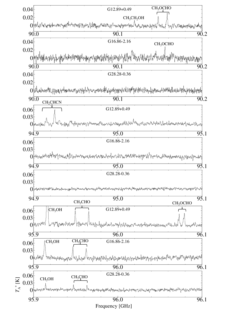
Figure 5: Spectra of the complex organic molecules in the 90.0$-$90.2, 94.9$-$95.1, and 95.9$-$96.1 GHz bands in the three sources obtained with the Nobeyama 45-m telescope.

Table 6: Summary of detection of complex organic molecules in the three sources with the Nobeyama 45-m telescope

Species	G12.89+0.49	G16.86$-$2.16	G28.28$-$0.36
CH3OCHO	Y	Y	N
CH3CH2OH	Y	N	N
CH3CHO	Y	Y	Y
CH3OCH3	Y	N	N
NH2CHO	Y	N	N
CH2CHCN	Y	N	N
CH3CH2CN	Y	N	N

Note. — ‘Y’ and ‘N’ represent detection and non-detection with a S/N ratio above 4, respectively.

3.2 Observational Results with the ASTE 10-m Telescope

Figure 6 shows the spectra in the 338.2$-$339.2 and 348.45$-$349.45 GHz bands obtained with the ASTE 10-m telescope. Table 7 summarizes the spectral line parameters obtained from the Gaussian fitting. The detection limit was set at a S/N ratio above 4. The $V_{\rm{LSR}}$ values are consistent with the systemic velocities of each source (Table 2). Several high-excitation energy ($E_{\rm{u}}/k>200$ K) lines from CH₃OH and CH₃CN were detected from G12.89+0.49. On the other hand, only two lower-excitation energy ($E_{\rm{u}}/k<75$ K) lines of CH₃OH and CCH were detected from G28.28$-$0.36. The line density in G16.86$-$2.16 is between those in G12.89+0.49 and G28.28$-$0.36. The relatively high-excitation energy line of CH₃OH ($7_{4,3}-6_{4,2}$ $A^{+}$ transition; $E_{\rm{u}}/k=145.3$ K) was detected in G16.86$-$2.16. The results suggest that hot gas exists in G12.89+0.49 and G16.86$-$2.16, which is supported by the detection of the metastable inversion transition NH₃ lines with the very-high-excitation energies, ($J,K$) = (8, 8) at 26.51898 GHz ($E_{\rm{u}}/k=686$ K) and ($J,K$) = (9, 9) at 27.47794 GHz ($E_{\rm{u}}/k=852$ K), with the GBT (Taniguchi et al., 2017b).

In G12.89+0.49 and G16.86$-$2.16, the line profiles of CH₃OH show wing emission suggestive of molecular outflow origins. In addition, the line widths (FWHM) of CH₃OH in these two sources ($\sim 5-6$ km s^-1) are larger than those in G28.28$-$0.36 ($\sim 2-3$ km s^-1). This may suggest that CH₃OH in G28.28$-$0.36 exists in less turbulent regions, as it is discussed in more detail in Section 5.6.

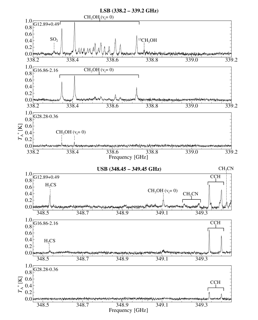
Figure 6: Spectra in the 338.2$-$339.2 and 348.45$-$349.45 GHz bands toward the three sources with the ASTE 10-m telescope.

Table 7: Spectral line parameters in the three sources with the ASTE 10-m telescope

			G12.89+0.49					G16.86$-$2.16					G28.28$-$0.36
Species &	Frequency	$E_{\rm{u}}/k$	$T_{\rm{mb}}$	FWHM	$\int T_{\mathrm{mb}}dv$	$V_{\rm{LSR}}$		$T_{\rm{mb}}$	FWHM	$\int T_{\mathrm{mb}}dv$	$V_{\rm{LSR}}$		$T_{\rm{mb}}$	FWHM	$\int T_{\mathrm{mb}}dv$	$V_{\rm{LSR}}$
Transition	(GHz)	(K)	(K)	(km s-1)	(K km s-1)	(km s-1)		(K)	(km s-1)	(K km s-1)	(km s-1)		(K)	(km s-1)	(K km s-1)	(km s-1)
SO2
$18_{4,14}-18_{3,15}$	338.305993	196.8	0.13 (4)	5.9 (9)	0.81 (9)	33.1		$<0.09$	…	…	…		$<0.09$	…	…	…
CH3OH
$7_{-1,7}-6_{-1,6}$ $E$	338.344628	70.5	1.23 (4)	4.6 (9)	5.99 (10)	32.9		0.82 (3)	4.5 (9)	3.94 (8)	17.3		0.17 (3)	2.2 (8)	0.40 (6)	48.9
$7_{0,7}-6_{0,6}$ $A^{+}$	338.408681	65.0	1.50 (4)	5.1 (9)	8.06 (11)	33.0		1.07 (3)	4.8 (9)	5.42 (7)	17.2		0.19 (3)	2.5 (8)	0.49 (5)	49.2
$7_{-6,1}-6_{-6,0}$ $E$	338.430933	253.9	0.23 (4)	5.8 (9)	1.40 (9)	32.9		$<0.09$	…	…	…		$<0.09$	…	…	…
$7_{6,1}-6_{6,0}$ $A^{+}$	338.442344	258.7	0.26 (4)	4.5 (9)	1.22 (9)	33.0		$<0.09$	…	…	…		$<0.09$	…	…	…
$7_{-5,2}-6_{-5,1}$ $E$	338.456499	189.0	0.26 (4)	5.0 (9)	1.38 (11)	32.9		$<0.09$	…	…	…		$<0.09$	…	…	…
$7_{5,3}-6_{5,2}$ $E$	338.475290	201.1	0.25 (4)	5.2 (9)	1.42 (11)	32.7		$<0.09$	…	…	…		$<0.09$	…	…	…
$7_{5,3}-6_{5,2}$ $A^{+}$	338.486337	202.9	0.25 (4)	5.9 (9)	1.55 (11)	33.2		$<0.09$	…	…	…		$<0.09$	…	…	…
$7_{-4,4}-6_{-4,3}$ $E$	338.504099	152.9	0.30 (4)	6.0 (9)	1.91 (10)	32.8		$<0.09$	…	…	…		$<0.09$	…	…	…
$7_{4,3}-6_{4,2}$ $A^{+}$	338.512627	145.3	0.51 (4)	4.7 (9)	2.56 (11)	32.7		0.14 (3)	6.1 (9)	0.92 (10)	17.7		$<0.09$	…	…	…
$7_{4,3}-6_{4,2}$ $E$	338.530249	161.0	0.27 (4)	6.0 (9)	1.72 (9)	32.8		$<0.09$	…	…	…		$<0.09$	…	…	…
$7_{3,5}-6_{3,4}$ $A^{+}$	338.540795	114.8	0.56 (4)	6.1 (9)	3.64 (12)	32.0		0.15 (3)	6.7 (9)	1.10 (10)	16.1		$<0.09$	…	…	…
$7_{-3,5}-6_{-3,4}$ $E$	338.559928	127.7	0.36 (4)	4.5 (9)	1.73 (10)	32.8		$<0.09$	…	…	…		$<0.09$	…	…	…
$7_{3,4}-6_{3,3}$ $E$	338.583195	112.7	0.36 (4)	5.2 (9)	2.00 (10)	33.0		$<0.09$	…	…	…		$<0.09$	…	…	…
$7_{1,6}-6_{1,5}$ $E$	338.614999	86.1	0.73 (4)	5.5 (9)	4.28 (11)	33.3		0.26 (3)	4.3 (9)	1.20 (8)	17.3		$<0.09$	…	…	…
$7_{2,5}-6_{2,4}$ $A^{+}$	338.639939	102.7	0.45 (4)	4.9 (9)	2.36 (11)	33.2		0.12 (3)	5.8 (9)	0.72 (9)	17.9		$<0.09$	…	…	…
$7_{-2,6}-6_{-2,5}$ $E$	338.72294	90.9	0.89 (4)	4.9 (9)	4.64 (11)	32.3		0.51 (3)	5.8 (9)	3.10 (7)	18.2		$<0.09$	…	…	…
$14_{1,13}-14_{0,14}$ $A^{-+}$	349.10702	260.2	0.36 (4)	6.0 (9)	2.29 (12)	33.2		$<0.09$	…	…	…		$<0.09$	…	…	…
13CH3OH
$13_{0,13}-12_{1,12}$ $A^{+}$	338.759948	205.9	0.17 (4)	4.5 (9)	0.80 (6)	33.0		$<0.09$	…	…	…		$<0.09$	…	…	…
H2CS
$10_{1,9}-9_{1,8}$	348.5343647	105.2	0.55 (4)	4.5 (9)	2.64 (11)	32.9		0.10 (3)	6.2 (9)	0.64 (6)	17.4		$<0.09$	…	…	…
CCH
$N=4-3,J=9/2-7/2$	349.3374558	41.9	1.17 (4)	4.2 (9)	5.22 (11)	33.7		1.12 (3)	3.2 (9)	3.82 (8)	16.8		0.34 (3)	3.4 (9)	1.25 (7)	48.1
$N=4-3,J=7/2-5/2$	349.3992738	41.9	0.80 (4)	3.8 (9)	3.27 (11)	32.1		0.86 (3)	3.3 (9)	3.04 (8)	17.1		0.25 (3)	3.4 (9)	0.92 (7)	48.3
CH3CN
$J_{K}=19_{6}-18_{6}$	349.2123106	424.7	0.14 (4)	5.4 (9)	0.81 (12)	33.1		$<0.09$	…	…	…		$<0.09$	…	…	…
$J_{K}=19_{5}-18_{5}$	349.2860057	346.2	0.16 (4)	5.8 (9)	0.98 (12)	33.9		$<0.09$	…	…	…		$<0.09$	…	…	…
$J_{K}=19_{4}-18_{4}$	349.3463428	282.0	0.20 (4)	5.1 (9)	1.07 (11)	33.3		$<0.09$	…	…	…		$<0.09$	…	…	…
$J_{K}=19_{2}-18_{2}$	349.4268497	196.3	0.23 (4)	5.3 (9)	1.32 (11)	33.0		$<0.09$	…	…	…		$<0.09$	…	…	…

Note. — Numbers in the parentheses are the standard deviation, expressed in units of the last significant digits. The upper limits correspond to the $3\sigma$ limits.

4 Analyses

4.1 Rotational Diagram Analysis

We derived the rotational temperatures and beam-averaged column densities of HC₃N, CH₃CCH, and CH₃OH with the beam size of $18\arcsec$ in the three sources from the rotational diagram analysis, using the following formula (Goldsmith & Langer, 1999);

$${\rm{ln}}\frac{3k\int T_{\mathrm{mb}}dv}{8\pi^{3}\nu S\mu^{2}}={\rm{ln}}\frac{N}{Q(T_{\rm{rot}})}-\frac{E_{\rm{u}}}{kT_{\rm{rot}}},$$ (1)

where $k$ is the Boltzmann constant, $S$ is the line strength, $\mu$ is the permanent electric dipole moment, $N$ is the column density, and $Q(T_{\rm{rot}})$ is the partition function. The permanent electric dipole moments are 3.7312, 0.784, and 0.899 D for HC₃N, CH₃CCH, and CH₃OH, respectively. We used $\int T_{\mathrm{mb}}dv$ values summarized in Tables 3, 4, and 5.

Figure 7 shows the fitting results of HC₃N, CH₃CCH, and CH₃OH in the three sources. The errors include the Gaussian fitting errors, the uncertainties from the main beam efficiency of 10%, the chopper-wheel method of 10%, and pointing calibration error of 30%. The derived rotational temperatures and column densities are summarized in Table 8.

In the case of HC₃N, we added data of the $J=3-2$ transition obtained with the GBT (Table 3 in Taniguchi et al., 2017b). The beam sizes are different among the three transitions, $27\arcsec$, $37\arcsec$, and $18\arcsec$ for the $J=3-2$, $5-4$, and $10-9$, respectively. Assuming a small beam filling factor, we multiplied the integrated intensities of the GBT data by ($\frac{27\arcsec}{18\arcsec}$)² and the 45 GHz band data by ($\frac{37\arcsec}{18\arcsec}$)² for the correction of the different beam sizes (filled circles in Figure 7). The red lines are the best fitting results for $J=5-4$ without beam size correction and $J=10-9$ transitions, and the green lines show the fitting results for the three transitions with beam size correction. In the case of the fitting for the $J=5-4$ and $10-9$ transitions, the $1\sigma$ fluctuation in the integrated intensity causes unlikely large errors in the derived rotational temperature and column density (e.g., $T_{\rm{rot}}\sim 600$ K), and we do not include the errors in Table 8. All of the three transitions are better fitted with beam size correction. The fitting results imply that the spatial distribution of HC₃N is smaller than 18″, corresponding to $\sim 0.07-0.1$ pc radii at the source distances (Table 2), like in the case for HC₅N (Taniguchi et al., 2017b). Taniguchi et al. (2017b) derived the rotational temperatures of HC₅N with beam size correction to be $\sim 13-20$ K in the three sources. The different rotational temperatures between HC₃N and HC₅N probably arise from the fact that we observed only lower excitation-energy lines ($E_{\rm{u}}/k<24.0$ K), compared to HC₅N ($E_{\rm{u}}/k\leq 100$ K; Taniguchi et al., 2017b), and the presence of complex excitation conditions.

In the case of CH₃CCH, we multiplied the integrated intensities of the $J=6-5$ transition lines by ($\frac{85.4{\rm GHz}}{102.5{\rm GHz}}$)² in order to correct the values for the $18\arcsec$ beam size at the 85 GHz band in G12.89+0.49 and G16.86$-$2.16, because data of the $J=6-5$ transition are systematically higher than those of the $J=5-4$ transition. In Figure 7, open and filled circles represent the integrated intensities without and with correction of frequency dependence of the beam size, respectively. The black lines show the fitting results with correction of frequency dependence. All of the data can be fitted simultaneously, which means that the spatial distribution of CH₃CCH is smaller than $18\arcsec$. This is the same case as for HC₃N and HC₅N. The derived rotational temperatures are $33^{+20}_{-9}$, $29^{+15}_{-8}$, and $23^{+9}_{-6}$ K in G12.89+0.40, G16.86$-$2.16, and G28.28$-$0.36, respectively.

In the case of CH₃OH, we fitted the data using all the lines in the 85$-$98 GHz band summarized in Table 5, and the fitting results are shown by the black lines in Figure 7. As is the case of CH₃CCH, we derived beam-averaged column densities a beam size of $18\arcsec$, correcting the frequency dependence of the beam size by multiplying the integrated intensities of the lines in the 95$-$98 GHz by ($\frac{85{\rm GHz}}{\nu{\rm GHz}}$)², where $\nu$ is the frequency of each line. The rotational temperatures are $42^{+33}_{-13}$, $36^{+18}_{-9}$, and $18^{+5}_{-3}$ K in G12.89+0.49, G16.86$-$2.16, and G28.28$-$0.36, respectively (Table 8). Purcell et al. (2009) derived the rotational temperatures of CH₃OH to be $5\pm 0.8$, $6\pm 0.1$, and $5\pm 0.5$ K in G12.89+0.49, G16.86$-$2.16, and G28.28$-$0.36, respectively, from fitting only three or four line transitions, which was interpreted as CH₃OH being sub-thermally excited. This does not seem to be the case when considering more CH₃OH transitions in the derivation of the rotational temperature.

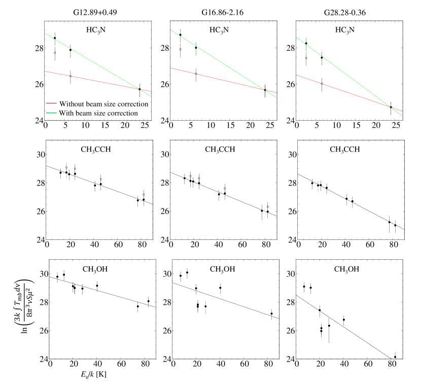
Figure 7: Rotational diagram of HC₃N, CH₃CCH, and CH₃OH in the three sources. HC₃N (upper panels): The filled and open circles represent with and without beam size correction, respectively. The red line is the fitting results for the $J=5-4$ data without beam size correction and $J=10-9$ data. The green line shows the fitting results for all of the lines with the beam size correction. CH₃CCH (middle panels): The filled and open circles represent with and without correction of frequency dependence, respectively. The black lines show the fitting results with correction of frequency dependence. CH₃OH (lower panels): The black lines show the fitting results for all of the observed lines.

Table 8: The rotational temperatures and beam-averaged column densities of HC₃N, CH₃CCH, and CH₃OH

	G12.89+0.49			G16.86$-$2.16			G28.28$-$0.36
Species	$T_{\rm{rot}}$	$N$		$T_{\rm{rot}}$	$N$		$T_{\rm{rot}}$	$N$
	(K)	(cm-2)		(K)	(cm-2)		(K)	(cm-2)
HC3N
$J=5-4$ & $10-9$	$24$	$4.4\times 10^{13}$		$20$	$4.3\times 10^{13}$		$13.4$	$2.0\times 10^{13}$
All	$7.7^{+1.6}_{-2.8}$	($1.4\pm 0.3$)$\times 10^{14}$		$7.2^{+1.4}_{-2.4}$	($1.3\pm 0.3$)$\times 10^{14}$		$6.2^{+1.1}_{-1.7}$	($7.6\pm 2.1$)$\times 10^{13}$
CH3CCH	$33^{+20}_{-9}$	$1.0^{+0.11}_{-0.02}\times 10^{15}$		$29^{+15}_{-8}$	$5.4^{+0.7}_{-0.8}\times 10^{14}$		$23^{+9}_{-6}$	$3.7^{+0.5}_{-0.9}\times 10^{14}$
CH3OH	$42^{+33}_{-13}$	$2.9^{+1.9}_{-1.3}\times 10^{15}$		$36^{+18}_{-9}$	$1.5^{+0.9}_{-0.7}\times 10^{15}$		$18^{+5}_{-3}$	$2.3^{+1.6}_{-1.1}\times 10^{14}$

Note. — The errors represent the standard deviation.

4.2 Column Densities of the D and ¹³C Isotopologues of HC₃N

We derived the column densities of the D and ¹³C isotopologues of HC₃N in the three sources assuming the LTE condition (Goldsmith & Langer, 1999). We used the following formulae;

$$\tau=-{\mathrm{ln}}\left[1-\frac{T_{\rm{mb}}}{J(T_{\rm{ex}})-J(T_{\rm{bg}})}\right]$$ (2)

where

$$J(T)=\frac{h\nu}{k}\Bigl{\{}\exp\Bigl{(}\frac{h\nu}{kT}\Bigr{)}-1\Bigr{\}}^{-1},$$ (3)

and

$$N=\tau\frac{3h\Delta v}{8\pi^{3}}\sqrt{\frac{\pi}{4\mathrm{ln}2}}Q\frac{1}{\mu^{2}}\frac{1}{J_{\rm{lower}}+1}\exp\Bigl{(}\frac{E_{\rm{lower}}}{kT_{\rm{ex}}}\Bigr{)}\Bigl{\{}1-\exp\Bigl{(}-\frac{h\nu}{kT_{\rm{ex}}}\Bigr{)}\Bigr{\}}^{-1}.$$ (4)

In Equation (2), $\tau$ denotes the optical depth, and $T_{\rm{mb}}$ the peak intensities summarized in Table 3. $T_{\rm{ex}}$ and $T_{\rm{bg}}$ are the excitation temperature and the cosmic microwave background temperature ($\simeq 2.73$ K). We used the rotational temperatures of HC₃N summarized in Table 8 as the excitation temperatures. We calculated two cases of excitation temperatures (Table 8) for each source. $J$($T$) in Equation (3) is the effective temperature equivalent to that in the Rayleigh-Jeans law. In Equation (4), N is the column density, $\Delta v$ is the line width (FWHM, Table 3), $Q$ is the partition function, $\mu$ is the permanent electric dipole moment, and $E_{\rm{lower}}$ is the energy of the lower rotational energy level. The electric dipole moments are 3.7408 D and 3.73172 D for DC₃N and the three ¹³C isotopologues, respectively. The derived column densities and the D/H and ¹²C/¹³C ratios are summarized in Table 9.

Table 9: The column densities of the D and ¹³C isotopologues of HC₃N

	G12.89+0.49			G16.86$-$2.16			G28.28$-$0.36
Species	$N$	D/H,		$N$	D/H,		$N$	D/H,
	(cm-2)	12C/13C		(cm-2)	12C/13C		(cm-2)	12C/13C
	$T_{\rm{ex}}=24$ K (fixed)			$T_{\rm{ex}}=20$ K (fixed)			$T_{\rm{ex}}=13.4$ K (fixed)
DC3N	$<6.2\times 10^{10}$	$<0.0014$		($5.5\pm 1.5$)$\times 10^{11}$	$0.013\pm 0.003$		($3.7\pm 1.0$)$\times 10^{11}$	$0.018\pm 0.005$
H13CCCN	($5.8\pm 1.7$)$\times 10^{11}$	$76\pm 23$		$<2.6\times 10^{11}$	$<165$		($6.8\pm 1.8$)$\times 10^{11}$	$30\pm 8$
HC13CCN	$<1.9\times 10^{11}$	$<237$		($7.6\pm 2.8$)$\times 10^{11}$	$57\pm 21$		($1.0\pm 0.3$)$\times 10^{12}$	$20\pm 5$
HCC13CN	($7.1\pm 1.9$)$\times 10^{11}$	$63\pm 16$		($1.8\pm 0.4$)$\times 10^{12}$	$24\pm 5$		($8.2\pm 2.3$)$\times 10^{11}$	$25\pm 7$
	$T_{\rm{ex}}=7.7$ K (fixed)			$T_{\rm{ex}}=7.2$ K (fixed)			$T_{\rm{ex}}=6.2$ K (fixed)
DC3N	$<5.4\times 10^{11}$	$<0.0046$		($4.9\pm 1.4$) $\times 10^{12}$	$0.037\pm 0.010$		($3.3\pm 0.9$)$\times 10^{12}$	$0.043\pm 0.012$
H13CCCN	($2.5\pm 0.8$)$\times 10^{12}$	$46\pm 14$		$<1.2\times 10^{12}$	$<114$		($3.1\pm 0.8$)$\times 10^{12}$	$24\pm 7$
HC13CCN	$<8.2\times 10^{11}$	$<142$		($3.4\pm 1.3$)$\times 10^{12}$	$38\pm 14$		($4.7\pm 1.2$)$\times 10^{12}$	$16\pm 4$
HCC13CN	($3.1\pm 0.8$)$\times 10^{12}$	$37\pm 10$		($6.0\pm 1.4$)$\times 10^{12}$	$22\pm 5$		($3.9\pm 1.1$)$\times 10^{12}$	$19\pm 5$

Note. — The errors represent the standard deviation. The upper limits were derived using the $1\sigma$ noise level.

5 Discussion

In this section, we will discuss comparisons of the chemical composition among MYSOs using CH₃OH, CH₃CCH, and HC₅N, all of which are considered to be in the lukewarm envelopes (Table 8). In the following discussion, we assume that the spatial distributions of CH₃OH, CH₃CCH, and HC₅N are similar to each other. This assumption is based on the following results; the source sizes of both HC₅N and CH₃CCH seem to be smaller than $18\arcsec$ (see Taniguchi et al. (2017b) and Section 4.1), and the rotational temperatures of CH₃OH are comparable with those of CH₃CCH in our three sources. Nitrogen-bearing COMs are usually originated from hot cores (e.g., Bisschop et al., 2007), and thus we do not include them in discussion. We will also discuss the relationship between the line width and excitation energy of rotational lines of CH₃OH.

5.1 Comparisons of Fractional Abundances in the High-Mass Star-Forming Regions

We derived the fractional abundances of HC₃N, CH₃OH, and CH₃CCH, $X$($a$) = $N$($a$)/$N$(H₂), in the three sources. The H₂ column densities, $N$(H₂), in the three sources were derived by Taniguchi et al. (2017b). The $N$(H₂) values and the fractional abundances of HC₃N, CH₃OH, CH₃CCH, and HC₅N derived by Taniguchi et al. (2017b) are summarized in Table 10. The derived $X$(CH₃OH) values are $1.2^{+1.8}_{-0.9}\times 10^{-7}$, $8.8^{+11}_{-5.8}\times 10^{-8}$, and $4.6^{+7.0}_{-3.4}\times 10^{-8}$ in G12.89+0.49, G16.86$-$2.16, and G28.28$-$0.36, respectively. The $X$(CH₃CCH) values are derived to be $4.2^{+2.8}_{-2.2}\times 10^{-8}$, $3.2^{+1.9}_{-1.5}\times 10^{-8}$, and $7.6^{+5.2}_{-4.4}\times 10^{-8}$ in G12.89+0.49, G16.86$-$2.16, and G28.28$-$0.36, respectively. We derive the $X$(HC₃N) values for two cases, fitting results of two transitions and all transitions (Table 8). Figure 8 shows their fractional abundances in the three sources. All of the column densities including the molecular hydrogen were derived as beam-averaged values for a beam size of $18\arcsec$. More accurate column densities and fractional abundances can be obtained in the future via interferometric observations that resolve the size of the sources.

Although our sample is small, there seems to be an anti-correlation between $X$(CH₃OH) and $X$(HC₅N). G12.89+0.49 shows the highest $X$(CH₃OH) value and the lowest $X$(HC₅N) value among the three sources, while G28.28$-$0.36 shows the lowest $X$(CH₃OH) value and the highest $X$(HC₅N) value. We further discuss the relationship between HC₅N and CH₃OH in Section 5.2. The $X$(HC₃N) has a positive correlation with $X$(HC₅N), while a negative correlation with $X$(CH₃OH).

The $X$(CH₃CCH) values in the three sources are consistent within their $1\sigma$ errors, and we cannot find any clear correlations between HC₅N and CH₃CCH. According to the gas-grain-bulk three-phase chemical network simulation (Majumdar et al., 2016, 2017a, 2017b) results assuming that the temperatures are 20 and 30 K and the density is $10^{5}$ cm^-3, CH₃CCH is formed on the grains and desorbed non-thermally (Hasegawa & Herbst, 1993; Garrod et al., 2007). HC₅N is formed in the gas phase mainly by the neutral-neutral reaction of CN + C₄H₂ and the electron recombination reaction of H₂C₅N⁺. The neutral-neutral reaction is also a main formation pathway to HC₅N in the model by Chapman et al. (2009). Chapman et al. (2009) suggested that C₄H₂ is formed by the reaction of C₂H₂ + CCH. C₂H₂ can be formed in the gas phase from CH₄ (Hassel et al., 2008) and can be directly evaporated from grain mantles (Lahuis & van Dishoeck, 2000). Hence, the productions of CH₃CCH and HC₅N seem to be related to the grain-surface reactions even in the lukewarm envelopes ($T\sim 20-30$ K). No correlation between CH₃CCH and HC₅N may imply that there is no direct relationship between them, which is also indicated in the chemical network simulation.

Table 10: The $N$(H₂) and fractional abundances of CH₃OH, CH₃CCH, HC₃N, and HC₅N in the three sources

Source	$N$(H2)	$X$(CH3OH)	$X$(CH3CCH)	$X$(HC3N)	$X$(HC3N)	$X$(HC5N)
	($\times 10^{22}$ cm-2)	($\times 10^{-8}$)	($\times 10^{-8}$)	($\times 10^{-9}$)	($\times 10^{-9}$)	($\times 10^{-10}$)
G12.89+0.49	$2.4^{+2.5}_{-0.8}$	$12^{+18}_{-9}$	$4.2^{+2.8}_{-2.2}$	$1.8\pm 0.9$	$5.8^{+4.8}_{-3.6}$	$9.9^{+6.1}_{-5.4}$
G16.86$-$2.16	$1.7^{+1.0}_{-0.5}$	$8.8^{+11}_{-5.8}$	$3.2^{+1.9}_{-1.5}$	$2.5^{+1.1}_{-0.9}$	$7.7^{+5.7}_{-3.9}$	$16\pm 7$
G28.28$-$0.36	$0.49^{+0.42}_{-0.16}$	$4.6^{+7.0}_{-3.4}$	$7.6^{+5.2}_{-4.4}$	$4.1^{+2.0}_{-1.9}$	$16^{+14}_{-9.5}$	$42^{+26}_{-20}$

Note. — The errors represent the standard deviation. These values are averaged ones with the beam size of $18\arcsec$.

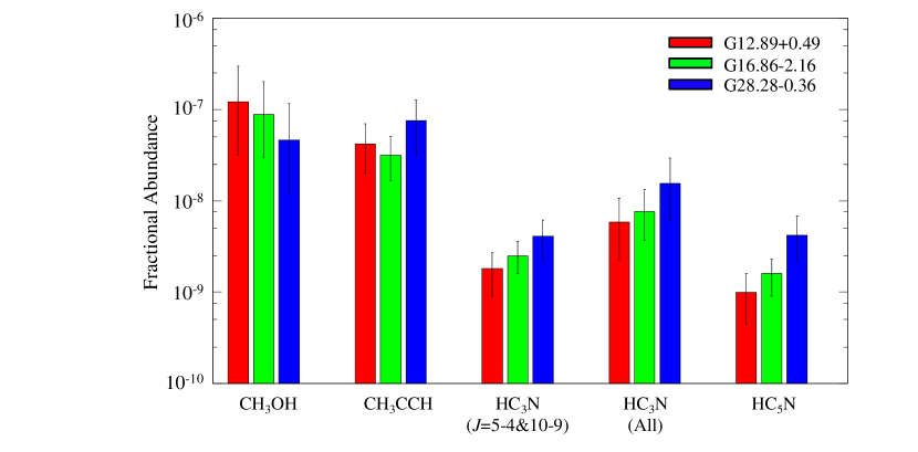
Figure 8: Fractional abundances of CH₃OH, CH₃CCH, HC₃N, and HC₅N in the high-mass star-forming regions. The HC₅N values are taken from Taniguchi et al. (2017b).

5.2 A Variety of the $N$(HC₅N)/$N$(CH₃OH) Ratio

Taniguchi et al. (2017b) found that the $N$(HC₅N)/$W$(CH₃OH) ratio, where $W$ represents the integrated intensity, varies by more than one order of magnitude among the three sources, and suggested the possibility of the chemical differentiation. In this paper, we derived the CH₃OH column densities in the three sources, and then we calculated the $N$(HC₅N)/$N$(CH₃OH) ratios in the observed three sources, as shown in Figure 9. We also added the data toward the high-mass protostellar object NGC2264 CMM3 (Watanabe et al., 2015). Watanabe et al. (2015) derived $N$(HC₅N) and $N$(CH₃OH) to be ($2.5\pm 0.9$)$\times 10^{13}$ cm^-2 and ($1.8\pm 0.2$)$\times 10^{15}$ cm^-2, respectively. We took the cold component value for CH₃OH, because its rotational temperature ($24.3\pm 2.6$ K) is comparable with that of HC₅N ($25.8\pm 4.6$ K) in NGC2264 CMM3 (Watanabe et al., 2015).

The $N$(HC₅N)/$N$(CH₃OH) ratio in G28.28$-$0.36 ($0.091^{+0.109}_{-0.039}$) is higher than that in G12.89+0.49 ($0.008^{+0.008}_{-0.004}$) by one order of magnitude, and those in G16.86$-$2.16 ($0.019^{+0.017}_{-0.008}$) and NGC2264 CMM3 ($0.014^{+0.007}_{-0.006}$) by a factor of $\sim 5$.

As Taniguchi et al. (2017b) discussed, the HC₅N molecules can be formed from CH₄ (WCCC, Aikawa et al., 2008; Hassel et al., 2008) and/or C₂H₂ (Chapman et al., 2009), which could be evaporated from grain mantles. CH₃OH is mainly formed by the successive hydrogenation reaction of CO molecules on dust grains, while CH₄, may be C₂H₂ (Lahuis & van Dishoeck, 2000) as well, are formed by the hydrogenation reaction of C atoms on dust grains. Therefore, the chemical differentiation in the lukewarm envelope may reflect the different ice chemical composition among the MYSOs.

Our source sample was chosen from the HC₅N-detected source list by Green et al. (2014). HC₅N was not detected in more than half of the sources where Green et al. (2014) carried out observations. In addition, Taniguchi et al. (2018) detected HC₅N in half of high-mass protostellar objects in their source list. The $N$(HC₅N)/$N$(CH₃OH) ratio should cover a broader range of values than the presented here, when considering the HC₅N-undetected sources into consideration.

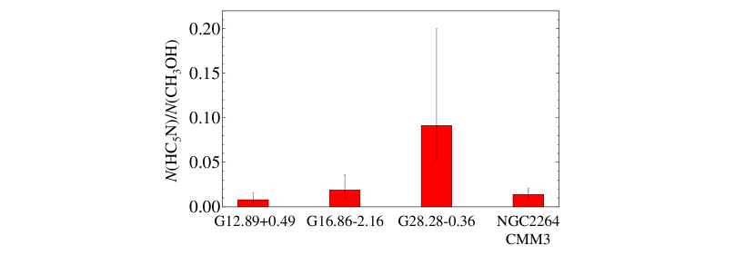
Figure 9: Comparison of the $N$(HC₅N)/$N$(CH₃OH) ratio among the three high-mass star-forming regions. The data for NGC2264 CMM3 were taken from Watanabe et al. (2015).

5.3 Relationship between $N$(HC₅N)/$N$(CH₃OH) and $N$(CH₃CCH)/$N$(CH₃OH)

In this subsection, we follow the analysis by Fayolle et al. (2015) who compared the chemical composition normalized by CH₃OH among MYSOs. We compare the chemical composition in the lukewarm envelope using the $N$(HC₅N)/$N$(CH₃OH) and $N$(CH₃CCH)/$N$(CH₃OH) ratios.

Figure 10 shows the relationship between the $N$(HC₅N)/$N$(CH₃OH) ratio and $N$(CH₃CCH)/$N$(CH₃OH) ratio in the four MYSOs, the observed three sources and NCG2264 CMM3 (Watanabe et al., 2015). The $N$(HC₅N)/$N$(CH₃OH) ratio correlates with the $N$(CH₃CCH)/$N$(CH₃OH) ratio. This is caused by the fraction of the lukewarm envelope in the single-dish beams, rather than the chemical differentiation. The chemical composition, based on HC₅N and CH₃CCH, of the lukewarm gas in G28.28$-$0.36 is similar to those in G16.86$-$2.16 and NGC2264 CMM3 (Ratio $\sim 20$). On the other hand, the $N$(CH₃CCH)/$N$(CH₃OH) ratio compared to the $N$(HC₅N)/$N$(CH₃OH) ratio in G12.89+0.49 is higher (Ratio $\approx 40$) than those in the other three sources. These results suggest the chemical diversity in the lukewarm envelope.

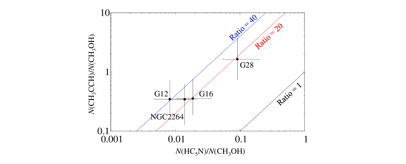
Figure 10: Plot of $N$(CH₃CCH)/$N$(CH₃OH) versus $N$(HC₅N)/$N$(CH₃OH). The data for NGC2264 CMM3 were taken from Watanabe et al. (2015). The labels of G12, G16, G28, and NGC2264 indicate the plots for G12.89+0.49, G16.86$-$2.16, G28.28$-$0.36, and NGC2264 CMM3, respectively.

5.4 Relationship of the Chemical Composition between Central Core and Envelope

He et al. (2012) carried out 1-mm spectral line survey observations toward 89 GLIMPSE Extended Green Objects (EGOs; Cyganowski et al., 2008). From their survey observations, there are largely two types of EGO clouds; line-rich and line-poor sources. It is unclear why some sources show line-poor spectra, and others show many lines of COMs. Ge et al. (2014) suggested that the EGO cloud cores are possibly in the short onset phase of the hot core stage, when CH₃OH ice is quickly evaporating from grain surfaces at a gas temperature of $\sim 100$ K. Hence, the difference between the line-poor and line-rich EGO cloud cores seems to originate from the chemical differentiation rather than the chemical evolution. Besides, Fayolle et al. (2015) compared the chemistry between organic-poor MYSOs and organic-rich MYSOs, namely hot cores, but the relationship between the central core and the envelope was not clear. In this subsection, we discuss a possibility of the relationship of the chemical composition between the core and the envelope.

There are clear differences in the spectra among the three sources (Figures 4 $-$ 6). As summarized in Table 6, the detected COMs are different among the three observed sources. CH₃CHO was detected toward all of the three sources, and it is considered to exist in the envelope (Fayolle et al., 2015). In G12.89+0.49, the largest number of COMs have been detected, while G28.28$-$0.36 is a line-poor source. The results in G28.28$-$0.36, a line-poor source, are consistent with those of He et al. (2012), showing that only H¹³CO⁺ was detected in G28.28$-$0.36. As discussed in Section 5.2, the $N$(HC₅N)/$N$(CH₃OH) ratio in G28.28$-$0.36 is higher than that in G12.89+0.49 by an order of magnitude. In the case of G16.86$-$2.16, the $N$(HC₅N)/$N$(CH₃OH) ratio shows a value between G12.89+0.49 and G28.28$-$0.36, and the line density and the COM’s line intensities are also between the others. From these results, the line-poor MYSOs are likely to be surrounded by the carbon-chain-rich envelope, while the line-rich MYSOs, namely hot cores, appear to be surrounded by the CH₃OH-rich envelope.

5.5 Isotopic Fractionation of HC₃N

The ¹²C/¹³C ratio shows a gradient with distance from the Galactic center ($D_{\rm{GC}}$; e.g., Savage et al., 2002; Milam et al., 2005). Recent observations derived the following relationship (Halfen et al., 2017);

$$^{12}{\rm{C}}/^{13}{\rm{C}}=5.21(\pm 0.52)D_{\rm{GC}}+22.6(\pm 3.3),$$ (5)

where $D_{\rm{GC}}$ is in units of kpc. We estimated the $D_{\rm{GC}}$ values of each source using trigonometry. The $D_{\rm{GC}}$ values are estimated at 5.8 and 8.9 kpc for G12.89+0.49 and G16.86$-$2.16, respectively. The $D_{\rm{GC}}$ value of G28.28$-$0.36 was derived to be 5.4 kpc by Taniguchi et al. (2016b). From Equation (5), the ¹²C/¹³C ratios are calculated at $53\pm 6$, $69\pm 8$, and $51\pm 6$ in G12.89+0.49, G16.86$-$2.16, and G28.28$-$0.36, respectively.

The ¹²C/¹³C ratios derived from observations (Table 9) are generally lower than or consistent with the values calculated from Equation (5) within the errors, except for non-detection species. These results mean that the ¹³C species of HC₃N are not heavily diluted. The ¹²C/¹³C ratios of cyanopolyynes in dark clouds (e.g., TMC-1, L1521B, and L134N; Taniguchi et al., 2016a, 2017a) are generally lower than those of other carbon-chain species (e.g., CCH, CCS, C₃S, C₄H), which means that the ¹³C species of cyanopolyynes are not heavily diluted. Similar results with the ¹²C/¹³C ratios of HC₃N being not significantly high were also found in the warm gas around the protostar L1527 (Taniguchi et al., 2016b). Our results show the similar tendency to the local low-mass star-forming regions.

Belloche et al. (2016) reported a tentative detection of DC₃N toward the Sgr B2 (N2) hot core and derived the D/H ratio to be 0.09%. A tentative detection of DC₃N was also achieved toward the Compact Ridge and the hot core of Orion KL (Esplugues et al., 2013), and the deuterium fractionation was estimated at $1.5\pm 0.9$%. The deuterium fractionation in the high-mass protostellar object NGC2264 CMM3 was calculated at $1.8\pm 1.5$% from a tentative detection of DC₃N (Watanabe et al., 2015). The higher D/H values were reported toward cold dense cores (5%$-$10%, Howe et al., 1994) and toward the L1527 protostar, which is one of the warm carbon chain chemistry sources ($\sim 3$%, Sakai et al., 2009b). The D/H values of HC₃N in G16.86$-$2.16 and G28.28$-$0.36 ($\sim 1-5$%) is higher than that in Sgr B2, lower than cold dense cores, and comparable to Orion KL hot core and L1527. On the other hand, DC₃N was not detected in G12.89+0.49 and we only derived the upper limit for its D/H ratio, which is significantly lower than those in G16.86$-$2.16 and G28.28$-$0.36. In general, the D/H ratio becomes lower in the higher temperature regions (e.g., Caselli & Ceccarelli, 2012). Hence, the results may imply that the emission of HC₃N comes from the G12.89+0.49 central hot core position, and the lukewarm envelope component is less than those in the other two sources. In the observations presented here, the lukewarm envelopes and the central cores were covered by the single-dish beam, and we cannot distinguish between them. The D/H ratio significantly depends on the temperature, and we need the high-spatial resolution observations using interferometers such as ALMA to derive the temperature dependence of the D/H ratio.

5.6 A Comparison of Line Width of CH₃OH

Line width is a key tool to characterize the environments where the molecules exist. In general, high-excitation energy lines are expected to trace the hotter gas and show broad line widths, whereas low-excitation energy lines come mainly from cold molecular clouds and show narrow line widths. We detected several CH₃OH emission lines with different excitation energies. We will investigate the relationship between the excitation energy and the line width of CH₃OH in this subsection.

Figure 11 shows a comparison between the line widths of CH₃OH and the excitation energy of each line. We derive the line width ($\Delta v$) using the following formula;

$$\Delta v=\sqrt{\Delta v_{\rm{obs}}^{2}-\Delta v_{\rm{inst}}^{2}},$$ (6)

where $\Delta v_{\rm{obs}}$ and $\Delta v_{\rm{inst}}$ are the observed line widths (Tables 5 and 7) and the instrumental velocity width (0.85 km s^-1 $-$ 0.86 km s^-1, Section 2), respectively.

We conducted the Kendall’s $\tau$ correlation coefficient test. The probability ($p$) that there is no correlation between the line width and the excitation energy is calculated at 0.03%, and the $\tau$ value is $+0.51$ in G12.89+0.49. This suggests the weak positive correlation between the line width and the excitation energy. The $p$ and $\tau$ values are derived to be 69% and $+0.08$ in G16.86$-$2.16, respectively. In G28.28$-$0.36, the $p$ and $\tau$ values are 72% and $-0.45$, respectively. Hence, there is no clear correlation between the line width and the excitation energy in G16.86$-$2.16 and G28.28$-$0.36. This may be caused by the non-detection of the very-high-excitation energy lines in the two sources.

We also compared the distributions of the CH₃OH line widths among the three sources using the two-sample Kolmogorov-Smirnov test (K-S test). We compared the distributions for all of the combinations; (a) G12.89+0.49 and G28.28$-$0.36, (b) G16.86$-$2.16 and G28.28$-$0.36, and (c) G12.89+0.49 and G16.86$-$2.16. The probabilities that the distributions of the line widths in the selected two sources are the same are derived to be $3.2\times 10^{-4}$%, $5.8\times 10^{-3}$%, and 39% for case (a), (b), and (c), respectively. These results mean that the distribution of the CH₃OH line width in G28.28$-$0.36 is clearly different from those in the other two sources, and we cannot exclude the possibility that the distributions in G12.89+0.49 and G16.86$-$2.16 are different.

The average line widths of CH₃OH are $4.8\pm 0.6$, $5.2\pm 0.6$, and $2.6\pm 0.5$ km s^-1 in G12.89+0.49, G16.86$-$2.16, and G28.28$-$0.36, respectively. Although the average line widths in G12.89+0.49 and G16.86$-$2.16 are consistent with each other within the errors, G16.86$-$2.16 shows the highest value; nevertheless the very-high-excitation energy lines were not detected in G16.86$-$2.16. These imply that CH₃OH exists in turbulent gas such as a molecular outflow in G16.86$-$2.16 rather than the hot gas. This is supported by the strong wing emission in the CH₃OH spectra in G16.86$-$2.16. In G12.89+0.49, CH₃OH seems to exist in the hot gas as well as in molecular outflow suggested by the wing emission. On the other hand, the line width in G28.28$-$0.36 is much narrower than those in the other two sources. This suggests that CH₃OH exists mainly in the relatively quiescent region, i.e. envelope for this source. The non-detection of the very-high-excitation energy lines is consistent with the envelope origin. There is a possibility of the molecular outflow origin, but a low S/N ratio prevents us from confirmation.

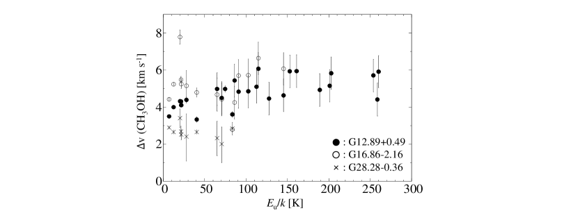
Figure 11: Relationship between excitation energy and line width of CH₃OH.

6 Conclusions

We carried out observations in the 42$-$46 and 82$-$103 GHz bands with the Nobeyama 45-m radio telescope, and in the 338.2$-$339.2 and 348.45$-$349.45 GHz bands with the ASTE 10-m telescope toward the three high-mass star-forming regions associated with the 6.7 GHz CH₃OH masers, G12.89+0.49, G16.86$-$2.16, and G28.28$-$0.36. The rotational temperatures and the beam-averaged column densities of HC₃N, CH₃CCH, and CH₃OH in the three sources are derived.

The $N$(HC₅N)/$N$(CH₃OH) ratio in G28.28$-$0.36 is higher than that in G12.89+0.49 by one order of magnitude and that in G16.86$-$2.16 by a factor of 5. Moreover, the relationships between the $N$(HC₅N)/$N$(CH₃OH) ratio and the $N$(CH₃CCH)/$N$(CH₃OH) ratio in G28.28$-$0.36 and G16.86$-$2.16 are similar to each other, while HC₅N is deficient when compared to CH₃CCH in G12.89+0.49. These results may imply the chemical diversity of the lukewarm envelope.

The line density in G28.28$-$0.36 is significantly low and a few COMs have been detected, while oxygen-/nitrogen-bearing COMs and high-excitation-energy lines have been detected from G12.89+0.49. These results seem to imply that the organic-poor MYSOs (G28.28-0.36) are surrounded by the carbon-chain-rich lukewarm envelope, whereas the organic-rich MYSOs (G12.89+0.49 and G16.86-2.16), hot cores, are surrounded by the CH₃OH-rich lukewarm envelope. The results presented in this paper were led based on observations with single-dish telescopes without information about the spatial distributions of each molecular emission and only a few molecular species. Further observations are required to confirm the trends reported in this work.

References

- Aikawa et al. (2008) Aikawa, Y., Wakelman, V., Garrod, R. T., & Herbst, E. 2008, ApJ, 674, 993
- Bacmann et al. (2012) Bacmann, A., Taquet, V., Faure, A., Kahane, C., & Ceccarelli, C. 2012, A&A, 541, L12
- Balucani et al. (2015) Balucani, N., Ceccarelli, C., & Taquet, V. 2015, MNRAS, 449, L16
- Belloche et al. (2016) Belloche, A., Müller, H. S. P., Garrod, R. T., & Menten, K. M. 2016, A&A, 587, A91
- Bisschop et al. (2007) Bisschop, S. E., Jørgensen, J. K., van Dishoeck, E. F., & de Wachter, E. B. M. 2007, A&A, 465, 913
- Caselli & Ceccarelli (2012) Caselli, P., & Ceccarelli, C. 2012, A&A Rev., 20, 56
- Cernicharo et al. (2012) Cernicharo, J., Marcelino, N., Roueff, E., et al. 2012, ApJ, 759, L43
- Chapman et al. (2009) Chapman, J. F., Millar, T. J., Wardle, M., Burton, M. G., & Walsh, A. J. 2009, MNRAS, 394, 221
- Cyganowski et al. (2008) Cyganowski, C. J., Whitney, B. A., Holden, E., et al. 2008, AJ, 136, 2391
- Esplugues et al. (2013) Esplugues, G. B., Cernicharo, J., Viti, S., et al. 2013, A&A, 559, A51
- Fayolle et al. (2015) Fayolle, E. C., Öberg, K. I., Garrod, R. T., van Dishoeck, E. F., & Bisschop, S. E. 2015, A&A, 576, A45
- Garrod et al. (2007) Garrod, R. T., Wakelam, V., & Herbst, E. 2007, A&A, 467, 1103
- Ge et al. (2014) Ge, J. X., He, J. H., Chen, X., & Takahashi, S. 2014, MNRAS, 445, 1170
- Goldsmith & Langer (1999) Goldsmith, P. F., & Langer, W. D. 1999, ApJ, 517, 209
- Green et al. (2014) Green, C. -E., Green, J. A., Burton, M. G., et al. 2014, MNRAS, 443, 2252
- Halfen et al. (2017) Halfen, D. T., Woolf, N. J., & Ziurys, L. M. 2017, ApJ, 845, 158
- Hasegawa & Herbst (1993) Hasegawa, T. I., & Herbst, E. 1993, MNRAS, 261, 83
- Hassel et al. (2008) Hassel, G. E., Herbst, E., & Garrod, R. T. 2008, ApJ, 681, 1385
- He et al. (2012) He, J. H., Takahashi, S., & Chen, X. 2012, ApJS, 202, 1
- Herbst & van Dishoeck (2009) Herbst, E., & van Dishoeck, E. F. 2009, ARA&A, 47, 427
- Hirota et al. (2009) Hirota, T., M. Ohishi, & Yamamoto, S 2009, ApJ, 699, 585
- Howe et al. (1994) Howe, D. A., Millar, T. J., Schilke, P., & Walmsley, C. M. 1994, MNRAS, 267, 59
- Iguchi & Okuda (2008) Iguchi, S., & Okuda, T. 2008, PASJ, 60, 857
- Imai et al. (2016) Imai, M., Sakai, N., Oya, Y., et al. 2016, ApJ, 830, L37
- Jaber et al. (2014) Jaber, A. A., Ceccarelli, C., Kahane, C., & Caux, E. 2014, ApJ, 791, 29
- Kamazaki et al. (2012) Kamazaki, T., Okumura, S. K., Chikada, Y., et al. 2012, PASJ, 64, 29
- Lahuis & van Dishoeck (2000) Lahuis, F., & van Dishoeck, E. F. 2000, A&A, 355, 699
- Li et al. (2016) Li, F. C., Xu, Y., Wu, Y. W., et al. 2016, AJ, 152, 92
- Majumdar et al. (2017a) Majumdar, L., Gratier, P., Andron, I., Wakelam, V., & Caux, E. 2017a, MNRAS, 467, 3525
- Majumdar et al. (2017b) Majumdar, L., Gratier, P., Ruaud, M., et al. 2017b, MNRAS, 466, 4470
- Majumdar et al. (2016) Majumdar, L., Gratier, P., Vidal, T., et al. 2016, MNRAS, 458, 1859
- Marcelino et al. (2007) Marcelino, N., Cernicharo, J., Agúndez, M., et al. 2007, ApJ, 665, L127
- Milam et al. (2005) Milam, S. N., Savage, C., Brewster, M. A., Ziurys, L. M., & Wyckoff, S. 2005, ApJ, 634, 1126
- Mller et al. (2005) Mller, H. S. P., Schlder, F., Stutzki, J., & Winnewisser, G. 2005, JMoSt, 742, 215
- Nakajima et al. (2013) Nakajima, T., Kimura, K., Nishimura, A., et al. 2013, PASP, 125, 252
- Nakamura et al. (2015) Nakamura, F., Ogawa, H., Yonekura, Y., et al. 2015, PASJ, 67, 117
- Öberg et al. (2010) Öberg, K. I., Bottinelli, S., Jørgensen, J. K., & van Dishoeck, E. F. 2010, ApJ, 716, 825
- Okuda & Iguchi (2008) Okuda, T., & Iguchi, S. 2008, PASJ, 60, 315
- Potapov et al. (2016) Potapov, A., Sánchez-Monge, Á., Schilke, P., et al. 2016, A&A, 594, A117
- Purcell et al. (2006) Purcell, C. R., Balasubramanyam, R., Burton, M. G., et al. 2006, MNRAS, 367, 553
- Purcell et al. (2009) Purcell, C. R., Longmore, S. N., Burton, M. G., et al. 2009, MNRAS, 394, 323
- Reboussin et al. (2014) Reboussin, L., Wakelam, V., Guilloteau, S., & Hersant, F. 2014, MNRAS, 440, 3557
- Reid et al. (2014) Reid, M. J., Menten, K. M., Brunthaler, A., et al. 2014, ApJ, 783, 130
- Ruaud et al. (2016) Ruaud, M., Wakelam, V., & Hersant, F. 2016, MNRAS, 459, 3756
- Sakai et al. (2009a) Sakai, N., Sakai, T., Hirota, T., Burton, M., & Yamamoto, S. 2009a, ApJ, 697, 769
- Sakai et al. (2008) Sakai, N., Sakai, T., Hirota, T., & Yamamoto, S. 2008, ApJ, 672, 371-381
- Sakai et al. (2009b) Sakai, N., Sakai, T., Hirota, T., & Yamamoto, S. 2009b, ApJ, 702, 1025
- Savage et al. (2002) Savage, C., Apponi, A. J., Ziurys, L. M., & Wyckoff, S. 2002, ApJ, 578, 211
- Shimajiri et al. (2015) Shimajiri, Y., Sakai, T., Kitamura, Y., et al. 2015, ApJS, 221, 31
- Suzuki et al. (1992) Suzuki, H., Yamamoto, S., Ohishi, M., et al. 1992, ApJ, 392, 551
- Taniguchi et al. (2017a) Taniguchi, K., Ozeki, H., & Saito, M. 2017a, ApJ, 846, 46
- Taniguchi et al. (2016a) Taniguchi, K., Ozeki, H., Saito, M., et al. 2016a, ApJ, 817, 147
- Taniguchi et al. (2017b) Taniguchi, K., Saito, M., Hirota, T., et al. 2017b, ApJ, 844, 68
- Taniguchi et al. (2016b) Taniguchi, K., Saito, M., & Ozeki, H. 2016b, ApJ, 830, 106
- Taniguchi et al. (2018) Taniguchi, K., Saito, M., Sridharan, T. K., & Minamidani, T. 2018, ApJ, 854, 133
- Tielens & Hagen (1982) Tielens, A. G. G. M., & Hagen, W. 1982, A&A, 114, 245
- Urquhart et al. (2013) Urquhart, J. S., Moore, T. J. T., Schuller, F., et al. 2013, MNRAS, 431, 1752
- van Dishoeck (2017) van Dishoeck, E. F. 2017, arXiv:1710.05940
- Vastel et al. (2014) Vastel, C., Ceccarelli, C., Lefloch, B., & Bachiller, R. 2014, ApJ, 795, L2
- Watanabe et al. (2015) Watanabe, Y., Sakai, N., López-Sepulcre, A., et al. 2015, ApJ, 809, 162