Is coherence catalytic?

Abstract

Quantum coherence, the ability to control the phases in superposition states is a resource, and it is of crucial importance, therefore, to understand how it is consumed in use. It has been suggested that catalytic coherence is possible, that is repeated use of the coherence without degradation or reduction in performance. The claim has particular relevance for quantum thermodynamics because, were it true, it would allow free energy that is locked in coherence to be extracted indefinitely. We address this issue directly with a careful analysis of the proposal by Åberg [1]. We find that coherence cannot be used catalytically, or even repeatedly without limit.

Keywords: Quantum coherence, quantum correlations, state discrimination, resource theory

1 Introduction

Quantum coherence provides the ability to control the phases in superposition states and as such is an essential element in the investigation and harnessing of quantum phenomena. Indeed it is the element that is at the very core of quantum phenomena, referred to by Feynman as “the only mystery” [2]. The thermodynamic significance of coherence has long been established, even if not fully understood; indeed the link between masers (or lasers), which are the quintessential sources of coherent light, and heat engines was made long ago [3, 4].

Coherence is a key component, perhaps the crucial distinguishing feature, of quantum thermodynamics and it is essential, therefore, to have a reliable account of it as a resource. Not to do so might lead to at best inaccuracies and at worst, the prediction of phenomena that violate physical laws.

The idea of catalytic coherence and its variants has been applied to a range of topics including the analysis of autonomous quantum machines [6]. In quantum thermodynamics, Åberg’s repeatable property has been applied to the problem of extracting work from quantum coherence [5] and, at a more formal level, the catalysis argument has been extended to general symmetries [7]. Recently, quantum catalysis has been employed in a study of measurement-based quantum heat engines [8]. Quantum catalysis has become an important part of the nascent field of quantum thermodynamics [9]. However, is widely acknowledged that for a system to act as a catalysis it must be returned to its initial state at the end of the process [10, 11, 12, 13]. It is readily apparent that this condition is not fulfilled in the processes treated by Åberg [1]. Ng et al. [14] make a case for considering approximate forms of catalysis on the grounds that all physical processes are approximate in some sense. But this misses the difference between what is possible in principle and technical limitations: even in the absence of technical limitations Åberg’s catalysis does not operate as a catalysis.

Here we present an analysis of a proposal by Åberg that coherence is catalytic [1] or, perhaps more accurately, that it is a resource that can be used repeatedly without degradation in performance [5]. We ask, specifically, whether the coherence in Åberg’s proposal is indeed catalytic or repeatable and show that it is neither. In fact we show that coherence is a finite resource that is expended through use in accord with previous studies of the degradation [15, 16, 17] and consumption [18] of coherence. Describing the use of coherence as catalytic, approximately catalytic, inexact catalysis or repeatable not only fails to capture this crucial property of coherence but suggests that the contrary is true.

We present a reanalysis of the Åberg proposal concentrating, in particular, on the role of correlations. Our key finding is that the qubits to which the coherence is transferred are, necessarily correlated and it is these correlations that limit the efficacy of repeated operations. If we consider each qubit independently then we do indeed find that they are in identical states but that these are correlated. In information theory it is common to speak of a sequence of systems being independent and identically distributed (i. i. d.) [19]. For Åberg’s scheme the qubit states are indeed identically distributed but they are not independent and so are not i. i. d..

To be completely clear, coherence is a strictly finite resource. Repeated use inevitably degrades and ultimately consumes it. Once eliminated the residual coherence source performs no better than one prepared randomly. In the Åberg proposal this is reflected in the complete destruction of reservoir coherence following a single and ultimately inevitable error in the transfer of the phase reference to a qubit.

2 Proposed scheme for catalytic coherence

We begin with a brief presentation of the proposal by Åberg for demonstrating catalytic coherence (CC) [1]. The main idea explored in CC is exemplified by the use of a resource in the form of a multilevel quantum system acting as an “energy reservoir” that is initially in the coherent superposition state

$$|{\eta_{L,l_{0}}}\rangle=\frac{1}{\sqrt{L}}\sum_{l=0}^{L-1}|{l_{0}+l}\rangle,$$ (1)

where $|{l_{0}+l}\rangle$ for $l\in\mathbb{Z}$ are reservoir energy eigenstates. The coherence we seek to utilise is held in the relative phases between the amplitudes for the $L$ states forming this superposition. Here the phase is 0, but we could store a phase $\theta$ in the more general state

$$|{\eta_{L,l_{0}},\theta}\rangle=\frac{1}{\sqrt{L}}\sum_{l=0}^{L-1}e^{il\theta}|{l_{0}+l}\rangle.$$ (2)

For simplicity we shall work with the state (1) but should keep in mind the fact that it is being used as phase or coherence reference for $\theta=0$.

We start with the general scheme but give, at the end of this section, a specific example, which might make the scheme a little clearer. The task we are required to perform is to prepare, repeatedly, coherent superpositions of two-level systems (qubits), corresponding, at least approximately, to the operation

$$U|{\psi_{0}}\rangle=a|{\psi_{0}}\rangle+b|{\psi_{1}}\rangle$$ (3)

on a sequence of two-level systems, where $|{\psi_{0}}\rangle$, $|{\psi_{1}}\rangle$ are system energy eigenstates and $U$ is a given unitary operator. The coherent phase in the reservoir state, in particular, is imprinted on the state as the relative phase of the amplitudes $a$ and $b$.

The process is analyzed in CC in terms of the quantum channels

$$\Phi_{\sigma,U}(\rho_{0})=\tr_{E}[V(U)\rho_{0}\otimes\sigma V(U)^{\dagger}]$$ (4)

$$\Lambda_{\rho_{0},U}(\sigma)=\tr_{S}[V(U)\rho_{0}\otimes\sigma V(U)^{\dagger}]\ ,$$ (5)

where $\tr$ denotes the trace operation. Here $\Phi_{\sigma,U}(\rho_{0})$ represents a channel that acts on system $S$ in state $\rho_{0}=|{\psi_{0}}\rangle\langle{\psi_{0}}|$ and $\Lambda_{\rho_{0},U}(\sigma)$ represents the complementary channel that acts on energy reservoir $E$ in state $\sigma$. Here, the operator $V(U)$ acts on the tensor product of the associated Hilbert spaces ${\cal H}_{S}\otimes{\cal H}_{E}$ and is defined by

$$V(U)=\sum_{n,n^{\prime}=0,1}|{\psi_{n}}\rangle\langle{\psi_{n}}|U|{\psi_{n^{\prime}}}\rangle\langle{\psi_{n^{\prime}}}|\otimes\Delta^{n^{\prime}-n}\ ,$$ (6)

and $\Delta^{k}$, which is called the “shift operator”, is defined by

$$\Delta^{k}=\sum_{j\in\mathbb{Z}}|{j+k}\rangle\langle{j}|\ .$$ (7)

Throughout we assume that $l_{0}$ in (1) is larger than the number of times the reservoir is used, so that the interaction does not access the reservoir ground state, $|{0}\rangle$. Hence we do not need to differentiate between the doubly-infinite and half-infinite reservoirs, nor employ “regenerating” cycles, as in CC.

A key result of CC is that if $\tr(\Delta^{a}\sigma)\approx 1$ for $a=-2,\ldots,2$ then

$$\Phi_{\sigma,U}(\rho_{0})\approx U\rho_{0}U^{\dagger}\ .$$ (8)

Another key result is that the expectation value $\langle{\Delta^{a}}\rangle$ is invariant under the action of the channel on the reservoir $E$ in the sense that

$$\langle{\Delta^{a}}\rangle=\tr(\Delta^{a}\sigma)=\tr[\Delta^{a}\Lambda_{\rho,U}(\sigma)]\ ,$$ (9)

for all values of $a$. These two results are the basis for arguing that the same channel can be used again on another system to perform the exactly the same coherent operation, as epitomised explicitly in CC by the statement [1]

$$\Phi_{\Lambda(\sigma),U}=\Phi_{\sigma,U}\ .$$ (10)

This line of reasoning leads to the conclusion in CC that the coherence resource represented by the reservoir is not degraded by its use, and the claim that coherence has a catalytic property as illustrated by phrases such as ‘coherence is catalytic in this model’ and ‘we only use the coherence catalytically and do not “spend” it at all’ [1].

Nevertheless, it is acknowledged in CC that the state of the reservoir $\sigma$ is changed by the channel $\Lambda_{\rho,U}$, i.e. $\Lambda_{\rho,U}(\sigma)\neq\sigma$. This unavoidable change in the reservoir has prompted other authors to use alternative descriptors in place of Åberg’s ‘catalysis’. For example, Korzekwa et al. prefer to use ‘repeatable’ to avoid any suggestion of an unchanging reservoir [5]. Their argument is that for the channel to be repeatable, the reservoir only needs to remain as useful as it was initially irrespective of any change in its state. A different choice is taken by Marvian and Lloyd who use the qualified description of ‘approximate catalysis’ [7]. To some extent the issue between these authors comes down to the meaning of the term ‘catalysis’; this discussion, although of interest, is not the point of our paper. For the interested reader, however, we give a few historical remarks below.

The presentation above is necessarily somewhat formal and an example calculation might be helpful. Let us suppose that the desired transformation is $|{\psi_{0}}\rangle\rightarrow|{+}\rangle=2^{-1/2}(|{\psi_{0}}\rangle+|{\psi_{1}}\rangle)$. The action unitary transformation acting on the first qubit and the energy reservoir produces the state

$$V(U)|{\psi_{0}}\rangle\otimes|{\eta_{L,l_{0}}}\rangle=\frac{1}{\sqrt{2}}\left(|{\psi_{0}}\rangle\otimes|{\eta_{L,l_{0}}}\rangle+|{\psi_{1}}\rangle\otimes\Delta^{-1}|{\eta_{L,l_{0}}}\rangle\right),$$ (11)

which is approximately the desired state. To see this we can find the state of the qubit by tracing over the energy reservoir to give the mixed state with density operator

$$\rho_{S}=\left(1-\frac{1}{2L}\right)|{+}\rangle\langle{+}|+\frac{1}{2L}|{-}\rangle\langle{-}|,$$ (12)

where $|{-}\rangle=2^{-1/2}(|{\psi_{0}}\rangle-|{\psi_{1}}\rangle)$ is the state that is orthogonal to the desired superposition. For large $L$ this is a very good approximation to the intended state.

The state of the energy reservoir following the interaction is changed from the pure state $|{\eta_{L,l_{0}}}\rangle$ to the mixed state with density operator

$$\rho_{E}=\frac{1}{2}\left(|{\eta_{L,l_{0}}}\rangle\langle{\eta_{L,l_{0}}}|+\Delta^{-1}|{\eta_{L,l_{0}}}\rangle\langle{\eta_{L,l_{0}}}|\Delta\right).$$ (13)

This state has clearly changed, although the change is very small; the fidelity of the post-interaction state with the initial state is

$$\langle{\eta_{L,l_{0}}}|\rho_{E}|{\eta_{L,l_{0}}}\rangle=1-\frac{1}{L}\left(1-\frac{1}{2L}\right),$$ (14)

which is close to unity for large $L$. The reservoir state has changed and in this sense the process is not catalytic. There are two senses in which the coherence appears to be catalytic and repeatable, however, and this is the point: firstly, the post-interaction state of the energy reservoir is a mixture of two states, $|{\eta_{L,l_{0}}}\rangle$ and $\Delta^{-1}|{\eta_{L,l_{0}}}\rangle$, each of which functions equally well as a source of coherence for future use and secondly repeated uses of the energy reservoir as a coherence source to act on a sequence of qubits will produce for each of them the same mixed state (12). This is the basis of the claims for catalysis and repeatability, and it is these claims that we address in this paper. We find, however, that these promising indications are misleading.

3 Independence versus quantum correlations

We have seen that the Åberg scheme creates qubits in the mixed state (12) but the single-qubit state, which appears naturally in the channel picture, is only part of the story. It is of the very essence of “catalysis” or “repeatability” that the coherence source should be used more than once, ideally many times. A full description of the state of the qubits includes, not just the single-qubit properties, but also any correlations that exist between them. These correlations mean that the properties of a collection of qubits that have drawn coherence from the reservoir are very different to those of uncorrelated qubits each in the state $\rho_{S}$. We demonstrate this point explicitly by considering first just two qubits, then a collection of $N$ qubits and contrast the properties of these with those of uncorrelated qubits.

3.1 Two qubits

We start by considering the action of our coherent transformation on a pair of qubits, each prepared initially in the ground state $|{\psi_{0}}\rangle$. Applying the unitary operation $V(U)$ to each in turn produces the state

$$V(U)\otimes V(U)|{\psi_{0}}\rangle|{\psi_{0}}\rangle|{\eta}\rangle = \frac{1}{4}\left[|{+}\rangle|{+}\rangle(\mathbbm{1}+\Delta^{-1})^{2}|{\eta}\rangle\right.$$ (15)

$$\quad+(|{+}\rangle|{-}\rangle+|{-}\rangle|{+}\rangle)(\mathbbm{1}-\Delta^{-2})|{\eta}\rangle$$

$$\qquad\left.+|{-}\rangle|{-}\rangle(\mathbbm{1}-\Delta^{-1})^{2}|{\eta}\rangle\right],$$

where $\mathbbm{1}$ is the identity operator and we have, for brevity, written $|{\eta}\rangle$ for the reservoir state and omitted the tensor-product symbols where there is no ambiguity. Here $V(U)\otimes V(U)$ is a short hand for

$$V(U)\otimes V(U) = \sum_{n,n^{\prime},m,m^{\prime}=0,1}|{\psi_{n}}\rangle\langle{\psi_{n}}|U|{\psi_{n^{\prime}}}\rangle\langle{\psi_{n^{\prime}}}|\otimes$$ (16)

$$\qquad\qquad|{\psi_{m}}\rangle\langle{\psi_{m}}|U|{\psi_{m^{\prime}}}\rangle\langle{\psi_{m^{\prime}}}|\otimes\Delta^{n^{\prime}-n+m^{\prime}-m}.$$

The resulting state of the two qubits is not separable and, in particular, is not simply $\rho_{S}\otimes\rho_{S}$. As a simple demonstration of this we give the probabilities for the outcomes of measurements on the two qubits in the $\{|{+}\rangle,|{-}\rangle\}$ basis. We find these to be

$$P(+,+) = 1-\frac{3}{4L}$$

$$P(+,-) = \frac{1}{4L}=P(-,+)$$

$$P(-,-) = \frac{1}{4L},$$ (17)

where we have used the expression

$$\langle{\eta}|\Delta^{a}|{\eta}\rangle=1-\frac{|a|}{L}\qquad|a|\leq L.$$ (18)

That there are correlations between the two qubits is clear from the fact that these probabilities do not factor into products. For comparison we give the products of the single-qubit probabilities:

$$P(+)\times P(+) = 1-\frac{1}{L}+\frac{1}{4L^{2}}$$

$$P(+)\times P(-) = \frac{1}{2L}-\frac{1}{4L^{2}}=P(-)\times P(+)$$

$$P(-)\times P(-) = \frac{1}{4L^{2}}.$$ (19)

These are the probabilities that would result if the channel picture were sufficient to describe two uses of the phase resource so that the two-qubit state was $\rho_{S}\otimes\rho_{S}$.

The number of reservoir energy eigenstates involved is intended to be large, so we can take the large $L$ limit of these probabilities. It is clear, in this limit, that on most occasions measurements of the two qubits will result in the value ‘$+$’, but it is when one or more ‘$-$’ value occurs that we see the significance of the correlations. In the absence of correlations, the probability for getting two ‘$-$’ outcomes is very small, $\sim L^{-2}$, but the Åberg scheme produces this outcome with a much higher probability, $\sim L^{-1}$. Indeed it is noteworthy that all three outcomes in which at least one ‘$-$’ occurs have the same probability. This reflects a general feature on the correlations in the Åberg scheme. To see this clearly we consider the properties of a larger number of qubits.

3.2 $N<L$ qubits

The correlations evident on our analysis of two qubits are yet more apparent and significant when we consider a larger number of qubits. For $N$ qubits (where $N<L$) the interaction produces the combined qubit-reservoir state

$$V(U)^{\otimes N}|{\psi_{0}}\rangle^{\otimes N}|{\eta}\rangle=\left[\frac{1}{2}\left[|{+}\rangle(\mathbbm{1}+\Delta^{-1})+|{-}\rangle(\mathbbm{1}-\Delta^{-1})\right]\right]^{\otimes N}|{\eta}\rangle.$$ (20)

From this general expression we can extract the probabilities that a measurement on each of the $N$ qubits in the $\{|{+}\rangle,|{-}\rangle\}$ basis will give any chosen sequence of ‘$+$’ and ‘$-$’ results. The symmetry of the process means that the probability for any given sequence in which $n$ qubits are found in the state $|{+}\rangle$ and $N-n$ in the state $|{-}\rangle$ is

$$P_{\rm seq}(n)=\frac{1}{2^{2N}}\langle{\eta}|(\mathbbm{1}-\Delta)^{N-n}(\mathbbm{1}+\Delta)^{n}(\mathbbm{1}+\Delta^{-1})^{n}(\mathbbm{1}-\Delta^{-1})^{N-n}|{\eta}\rangle.$$ (21)

We emphasise that this probability does not depend on the order in which the qubits appear in this sequence as $\Delta$ commutes with $\Delta^{-1}$. This means, in turn, that the probability of finding $n$ of the qubits in the state $|+\rangle$ in any order is

$$P(n)=\left(\begin{array}[]{c}N\\ n\end{array}\right)P_{\rm seq}(n)\,,$$ (24)

and hence that the probabilities sum to unity, as they should:

$$\sum_{n=0}^{N}P(n) = \sum_{n=0}^{N}\left(\begin{array}[]{c}N\\ n\end{array}\right)2^{-2N}\langle\eta|(2\mathbbm{1}-\Delta-\Delta^{-1})^{N-n}(2\mathbbm{1}+\Delta+\Delta^{-1})^{n}|\eta\rangle$$

$$= \langle\eta|\left(\frac{\mathbbm{1}}{2}-\frac{\Delta}{4}-\frac{\Delta^{-1}}{4}+\frac{\mathbbm{1}}{2}+\frac{\Delta}{4}+\frac{\Delta^{-1}}{4}\right)^{N}|\eta\rangle$$

$$= 1\,.$$ (28)

Finding a single qubit in the state $|-\rangle$ leaves the reservoir in a state that is essentially devoid of the initial coherence and this suggests that the next qubit tested is equally likely to be found in the state $|-\rangle$ as in the state $|+\rangle$. This means to suggest, in particular, that

$$P_{\rm seq}(N-1)=P(0)\,,$$ (29)

so that, for example, if the first (or any other) qubit is found in the state $|-\rangle$ then the remaining $N-1$ are equally likely to all be found in the $|-\rangle$ or the state $|+\rangle$! The reason for this remarkable result is readily understood in terms of the state of the reservoir following a $|{-}\rangle$ outcome. In this case the reservoir state, $|{\eta}\rangle$, is acted on by $\mathbbm{1}-\Delta^{-1}$ and hence the (unnormalised) reservoir state becomes

$$(\mathbbm{1}-\Delta^{-1})|{\eta}\rangle=\frac{1}{\sqrt{L}}\left(|{l_{0}+L-1}\rangle-|{l_{0}-1}\rangle\right).$$ (30)

The are no adjacent or even nearby energy states in this case and hence it no longer acts as a source of coherence. Preparation from it of a $|{+}\rangle$ or a $|{-}\rangle$ state will happen with equal probability. More generally, the probability that the remaining qubits form a given sequence with $m$ qubits in the state $|{+}\rangle$ and $N-m-1$ in the state $|{-}\rangle$ is the same as that for a sequence in which $m$ qubits are found in the state $|{-}\rangle$ and $N-m-1$ in the state $|{+}\rangle$.

Evaluating the general probabilities $P_{\rm seq}(n)$ is a lengthy and not especially enlightening procedure, but we have found excellent approximations to these, which give probabilities to within a few percent or better for $N>1$. A few examples will suffice to indicate the trend:

$$P_{\rm seq}(N) = P(+,+,\cdots,+)$$

$$\approx 1-\sqrt{\frac{N}{\pi}}\frac{1}{L}$$

$$P_{\rm seq}(N-1) = P_{\rm seq}(0)=P(0)$$

$$\approx \frac{1}{2\sqrt{\pi(N-1)}L}$$

$$P_{\rm seq}(N-2) = P_{\rm seq}(1)$$

$$\approx \frac{1}{4\sqrt{\pi(N-2)^{3}}L}$$

$$P_{\rm seq}(N-3) = P_{\rm seq}(2)$$ (31)

$$\approx \frac{3}{8\sqrt{\pi(N-3)^{5}}L}.$$

The most striking feature of these probabilities is that those for which there is at least one ‘$-$’ outcome all fall off as $L^{-1}$. This contrasts strongly with the situation that would hold in the absence of the correlations, with the state $\rho_{S}^{\otimes N}$, for which $P_{\rm seq}(N-k)$ would fall off as $L^{-k}$. The overall probability that there will be $N-n\ll N$ ‘$-$’ outcomes is rather flat:

$$P(N-1) = NP_{\rm seq}(N-1)\approx\sqrt{\frac{N}{\pi}}\frac{1}{2L}$$

$$P(N-2) = \frac{N(N-1)}{2}P_{\rm seq}(N-2)\approx\sqrt{\frac{N}{\pi}}\frac{1}{8L}$$

$$P(N-3) = \frac{N(N-1)(N-2)}{6}P_{\rm seq}(N-3)\approx\sqrt{\frac{N}{\pi}}\frac{1}{16L},$$ (32)

where we have simplified these expressions by choosing $N\gg 1$. In the absence of these correlations, with the multi-qubit state $\rho_{S}^{\otimes N}$, the situation is very different and for $N\ll L$, it is most unlikely that more than one of the qubits will be found to be in the state ‘$-$’:

$$P_{\rho_{S}^{\otimes N}}(N-1)\approx\frac{N}{2L}$$

$$P_{\rho_{S}^{\otimes N}}(N-2)\approx\frac{1}{2}\left(\frac{N}{2L}\right)^{2}$$

$$P_{\rho_{S}^{\otimes N}}(N-3)\approx\frac{1}{6}\left(\frac{N}{2L}\right)^{3}.$$ (33)

For $N\ll L$ only the first of these is comparable to the probabilities for a small number of ‘$-$’ outcomes given in Eq. (3.2). The most extreme case is the probability that all the $N$ qubits will be found in the state $|{-}\rangle$ which, as we have seen, is approximately $(2L\sqrt{\pi N})^{-1}$, while for the uncorrelated state this probability has the vastly smaller value of $(2L)^{-N}$!

The correlations between the transformed qubits are a crucial part of the overall picture and although each qubit, when considered alone, will be found in the state $\rho_{S}$, the multi-qubit state is very different from the uncorrelated tensor product of these density operators. Multiple coherent operations, acting on multiple qubits is the very essence of catalysis and repeatability, and it follows that these correlations cannot be ignored. Neglecting these correlations can lead to unphysical conclusions as we demonstrate in the next section.

4 Paradoxical repercussions

The purpose of this section is to highlight the fundamental necessity for the existence of the correlations we have described and, in doing so, expose the inadequacy of describing each post-interaction qubit by the simple mixed state $\rho_{S}$. This is important as it shows that the requirement that we account fully for the correlations between the qubits is general and not simply a particular manifestation of the Åberg scheme.

4.1 Unphysical state discrimination

Our first example is one of quantum state discrimination [24, 25]. The key idea is that it is not possible, even in principle, to determine for certain in which of two known non-orthogonal quantum states a system has been prepared. The absolute minimum probability of error in making this choice is given by the Helstrom bound [26, 27].

Consider an energy reservoir to have been prepared in one of two possible initial states, $|{\eta(\theta_{1})}\rangle$ or $|{\eta(\theta_{2})}\rangle$ where

$$|{\eta(\theta)}\rangle=\frac{1}{\sqrt{L}}\sum_{l=0}^{L-1}e^{\rmi l\theta}|{l_{0}+l}\rangle.$$ (34)

In general these two possible reservoir states will not be orthogonal and if they are not orthogonal then it necessarily follows that we cannot discriminate between these two states with certainly.

Let us suppose that the energy reservoir is used to prepare a very large number of qubits, each of which will then be found in one of the mixed states

$$\rho(\theta_{j})=\frac{1}{2}\left[|{\psi_{0}}\rangle\langle{\psi_{0}}|+|{\psi_{1}}\rangle\langle{\psi_{1}}|+\left(1-\frac{1}{L}\right)(e^{-\rmi\theta_{j}}|{\psi_{0}}\rangle\langle{\psi_{1}}|+e^{\rmi\theta_{j}}|{\psi_{1}}\rangle\langle{\psi_{0}}|)\right],$$ (35)

where $j=1,2$. If we accept literally the claim of CC that the same reservoir can be used repeatedly to perform the same coherent operation and so create the state $\rho(\theta_{j})^{\otimes N}$ then we can recast the problem of determining the reservoir state as one of discriminating between the two $N$-qubit states, $\rho(\theta_{1})^{\otimes N}$ and $\rho(\theta_{2})^{\otimes N}$. The probability of error in discriminating between these two states decreases with each additional copy available, and approaches zero in the limit of large $N$. To show this explicitly, we note that the minimum achievable probability of error in discriminating two states $\rho$ and $\sigma$ is given by the well-known Helstrom bound [26, 27]:

$$P_{\rm err}(\rho,\sigma) =\frac{1}{2}\left(1-D(\rho,\sigma)\right)$$ (36)

where $D(\rho,\sigma)=\frac{1}{2}\tr|\rho-\sigma|$ is the trace distance. Further, a bound on the trace distance is given by $D(\rho,\sigma)\geq 1-F(\rho,\sigma),$ where $F(\rho,\sigma)=\tr\sqrt{\rho^{1/2}\sigma\rho^{1/2}}$ is the fidelity [28], thus

$$P_{\rm err}\leq\frac{1}{2}F(\rho,\sigma)\ .$$ (37)

For the $N$-copy states corresponding to different reservoir states the fidelity is readily calculated to be:

$$F(\rho(\theta_{1})^{\otimes N},\rho(\theta_{2})^{\otimes N}) =F(\rho(\theta_{1}),\rho(\theta_{2})])^{N}$$ (38)

$$=\left[1-\frac{1}{2}\left(1-\frac{1}{L}\right)^{2}\left(1-\cos(\theta_{1}-\theta_{2})\right)\right]^{\frac{N}{2}},$$

which tends to zero exponentially as $N$ increases. It would appear, therefore, that the channel could be used to discriminate between two non-orthogonal reservoir states $|{\eta_{L,l_{0}}(\theta_{1})}\rangle$, $|{\eta_{L,l_{0}}(\theta_{2})}\rangle$ with an accuracy approaching 100% [24, 29]. But this contradicts the fundamental result that no quantum measurement can unambiguously distinguish between two non-orthogonal states [27, 28]. Hence, we are left with a paradox: the results of CC—and (8), (9) and (10) in particular—appear to imply that the channel $\Phi_{\sigma,U}$ can perform coherent operations repeatedly, and yet we have just seen that this possibility would lead to a violation of a fundamental result in quantum measurement theory. The resolution, of course, lies in the correlations between the qubits that are neglected in the channel picture.

4.2 Unphysical generation of unbounded coherence

Our second example raises the issue of quantum coherence as a limited resource and so challenges directly the idea of its catalytic use. We start by noting that the coherence represented by the reservoir state in (1) is an example of a broken U(1) symmetry, and its coherence is quantified by its asymmetry with respect to the U(1) symmetry group. The asymmetry quantified by $A_{G}(\varrho)$ was first introduced by one of us [30, 31] as a measure of the ability of a system with density operator $\varrho$ to act as a reference and break the superselection rule (SSR) associated with a symmetry described by the group $G$. It is defined as [30, 31]

$$A_{G}(\varrho)\equiv S({\cal G}_{G}[\varrho])-S(\varrho)$$ (39)

where $S(\varrho)\equiv-\tr(\varrho\ln\varrho)$ is the von Neumann entropy of the density operator $\varrho$ and ${\cal G}_{G}[\cdot]$ is the twirl superoperator is given by

$$\mathcal{G}_{G}[\varrho]=\frac{1}{|G|}\sum_{g\in G}T_{g}\varrho T_{g}^{\dagger}$$ (40)

for the unitary representation $\{T_{g}:g\in G\}$ of a discrete group $G$ of order $|G|$. For continuous groups, the sum in (40) is replaced with an integral with an appropriate integration measure. The operational utility of $A_{G}(\varrho)$ is that it quantifies the extra work that is extractable from a quantum Szilard engine under a SSR when a system in the state $\varrho$ is used as a reference for the engine’s working fluid. In that case $k_{B}TA_{G}(\varrho)$, where $k_{B}$ is Boltzmann’s constant and $T$ is the temperature of the thermal reservoir, is an achievable upper bound on the extra work [30, 31]. The asymmetry $A_{G}(\varrho)$ has a number of other important properties [30, 31], but the salient one for us here is that it is non increasing under operations $\varrho\to\mathcal{O}[\varrho]$ that are $G$-covariant, i.e.

$$A_{G}(\mathcal{O}[\varrho])\leq A_{G}(\varrho)\ ,$$ (41)

where a $G$-covariant operation is one that satisfies $\mathcal{O}[T_{g}\varrho T^{\dagger}_{g}]=T_{g}\mathcal{O}[\varrho]T^{\dagger}_{g}$ for all $g\in G$.

In particular, the U(1) symmetry group

$${\rm U(1)}=\left\{T(\phi)=\exp\left(-\rmi{H_{0}\over s}\phi\right):0<\phi\leq 2\pi\right\}\ ,$$ (42)

is continuous and its corresponding twirl is given by

$${\cal G}_{\rm U(1)}[\varrho]=\int_{2\pi}\frac{d\phi}{2\pi}T(\phi)\varrho T^{\dagger}(\phi)$$ (43)

where $H_{0}=s\sum_{n}n|{n}\rangle\langle{n}|+s_{0}$ is the free Hamiltonian of the system, $s$ and $s_{0}$ represent an energy gap and “vacuum” energy parameters, respectively, and $\phi$ is a phase angle. This symmetry represents the invariance to phase rotations and $A_{\rm U(1)}(\varrho)$ measures the phase coherence of $\varrho$ in terms of how $\varrho$ breaks the U(1) symmetry. The U(1)-covariant operations $\mathcal{O}[\cdot]$ satisfy

$$\mathcal{O}\left[\exp\left(-\rmi{H_{0}\over s}\phi\right)\varrho\exp\left(\rmi{{H_{0}}\over s}\phi\right)\right]=\exp\left(-\rmi{H_{0}\over s}\phi\right)\mathcal{O}[\varrho]\exp\left(\rmi{H_{0}\over s}\phi\right)$$ (44)

for all values of $\phi$ in a $2\pi$ interval. In other words, U(1)-covariant operations commute with the phase-shifting operation. If we apply this to the reservoir state $|{\eta_{L,l_{0}}}\rangle$ then we find

$$\mathcal{G}_{G}[|{\eta}\rangle\langle{\eta}|]=\frac{\mathbbm{1}}{L},$$ (45)

so that the asymmetry is $A_{G}[|{\eta}\rangle\langle{\eta}|]=\ln L$.

The findings of CC, and (10) in particular, suggest that the channel $\Phi_{\sigma,U}$ can produce an inexhaustible supply of systems in the state $\Phi_{\sigma,U}(\rho_{0})$ and this has implications for the non increasing property of asymmetry. To see this let the initial state of a collection of $N$ systems be $\rho_{0}^{\otimes N}$ where $\rho_{0}=|{\psi_{0}}\rangle\langle{\psi_{0}}|$, $U$ be given by (3) and the reservoir initially be in the state $\sigma=|{\eta_{L,l_{0}}}\rangle\langle{\eta_{L,l_{0}}}|$ given by (1). This yields $\sigma^{\prime}=\Lambda_{\rho_{0},U}(\sigma)$, $\sigma^{\prime\prime}=\Lambda_{\rho_{0},U}(\sigma^{\prime})$ etc. and, using (10), we find that $\rho_{0}^{\otimes k}$ is transformed to

$$\cdots\otimes\Phi_{\sigma^{\prime\prime},U}(\rho_{0})\otimes\Phi_{\sigma^{\prime},U}(\rho_{0})\otimes\Phi_{\sigma,U}(\rho_{0}) =\cdots\otimes\Phi_{\sigma,U}(\rho_{0})\otimes\Phi_{\sigma,U}(\rho_{0})\otimes\Phi_{\sigma,U}(\rho_{0})$$ (46)

$$=\cdots\otimes\rho\otimes\rho\otimes\rho$$ (47)

where $\rho$ is given by (35) with $\theta=0$, i.e.

$$\rho=\frac{1}{2}\left[|{\psi_{0}}\rangle\langle{\psi_{0}}|+|{\psi_{1}}\rangle\langle{\psi_{1}}|+\left(1-\frac{1}{L}\right)(|{\psi_{0}}\rangle\langle{\psi_{1}}|+|{\psi_{1}}\rangle\langle{\psi_{0}}|)\right]\ .$$ (48)

In A we show that the asymmetry of the collection of systems is given approximately by

$$A_{\rm U(1)}(\rho^{\otimes N})\approx\frac{1}{2}\ln\left(\frac{N\pi e}{2}\right)$$ (49)

for large $L$ in the limit of large $N$. Figure 1 shows that (49) is a good approximation even for relatively small values of $L$ and $N$. The fact that the right side of (49) diverges as $N$ tends to infinity implies that the reservoir can be used to generate a collection of systems in a state that has unbounded coherence. Yet this conflicts with the physical requirement that the asymmetry must be non-increasing under physical operations. Once again, the resolution lies in the correlations between the qubits that are omitted in the simple channel picture. It is clear that these correlations are a fundamental component of the final multi-qubit state.

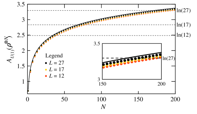
Figure 1: Comparison of the exact values of $A_{U(1)}(\rho^{\otimes N})$ (discs) with the approximate values given by (49) (continuous curve) for different values of $L$ and $N$. The red, yellow and black discs correspond to values of $A_{U(1)}(\rho^{\otimes N})$ for $L=12$, $17$ and $27$, respectively. For clarity, the discs are plotted for every third value of $N$ starting from $N=1$. Also plotted (as dotted grey lines) are the corresponding upper bounds on $A_{\rm U(1)}({\rm Tr}_{E}[{\cal V}_{N}(\rho_{0}^{\otimes N}\otimes\sigma)])$. The inset gives an enlarged view of the range $N=150$ to $200$.

5 Discussion and Conclusion

The validity of the key equations of CC, reproduced here as (8), (9) and (10), is not in dispute. These equations imply that each system $S_{i}$, if considered on its own (i.e. in the absence of information about the state of any other system $S_{j\neq i}$), will have a reduced density operator given by $\rho$ in (48). The fact that the reduced density operator is $\rho$—regardless of how many prior times the reservoir has been used to prepare other systems—may appear to be extraordinary. This situation simply reflects, however, the invariance of the single-system reduced density operator to the order in which the systems are prepared. This invariance is apparent in the commutativity of the operators $V_{i}(U)$ defined according to (6) for different systems $S_{i}$. For example, it is straightforward to see that $V_{1}(U)V_{2}(U)=V_{2}(U)V_{1}(U)$ and it follows that this commutability property generalises to any two systems $S_{i}$ and $S_{j}$. This leads to a crucial point: the dynamics of the interaction between the reservoir and the systems are invariant with respect to the ordering of the preparation of the systems.

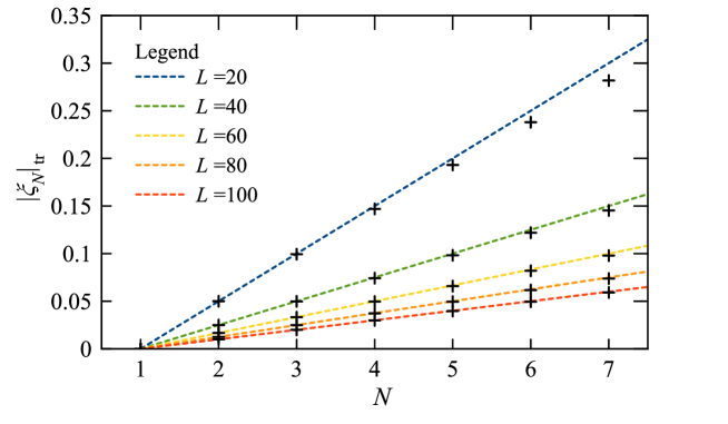
Figure 2: The trace norm of the repeatability error $\xi_{N}$ as a function of the number of systems $N$ for various values of $L$. The crosses represent exact values of $|\xi_{N}|_{\mbox{tr}}$ and the dashed lines represent the approximation $|\xi_{N}|_{\mbox{tr}}\approx(N-1)/L$ derived in B for $1\leq N\ll L$.

The invariance is the reason that every system prepared using the same reservoir, if considered on its own, has the same reduced density operator, $\rho$. It does not, however, imply that the preparation of the systems is catalytic or even repeatable, as claimed in CC. Rather, it merely implies that if one system is examined, it will be found to be in the state $\rho$ regardless of the order in which it is prepared. If, instead, two systems are examined, they will be found in the state $\tr_{E}[{\cal V}_{2}(\rho_{0}^{\otimes 2}\otimes\sigma)]$ regardless of the order in which they are prepared. To determine whether the preparation of a system is repeatable in the sense that another system is able to be prepared in the same state as the first, we need to compare the actual prepared state of both systems in question, i.e. $\tr_{E}[{\cal V}_{2}(\rho_{0}^{\otimes 2}\otimes\sigma)]$, with the state that represents both systems being prepared in the same state, i.e. $\rho^{\otimes 2}$. The fact that the state of two processed qubits is not $\rho^{\otimes 2}$ is a direct demonstration that the preparation is not repeatable. In general, the repeatability error in the preparation of $N$ systems is given by the difference $\xi_{N}=\tr_{E}[{\cal V}_{N}(\rho_{0}^{\otimes N}\otimes\sigma)]-\rho^{\otimes N}$. Figure 2 shows how the trace norm of $\xi_{N}$ grows linearly with $N$ for $1\leq N\ll L$. Given that it is the neglect of this error that leads to the paradoxical results discussed in preceding sections, it follows that the non-repeatability of the preparation cannot be ignored or even eliminated in principle—rather the non-repeatability of the preparation stands as a necessity for consistency with basic quantum principles. In conclusion, we can say, quite categorically, that coherence is not catalytic.

Appendix A Asymmetry of $\rho^{\otimes N}$

To derive a closed expression for the asymmetry

$$A_{\rm U(1)}(\rho^{\otimes N}) =S(\mathcal{G}_{\rm U(1)}[\rho^{\otimes N}])-S(\rho^{\otimes N})\ ,$$ (50)

where $\rho$ is given by (48) in the main text, we first deduce a number of preliminary results, as follows. In places we treat the energy eigenstates $|{\psi_{0}}\rangle$ and $|{\psi_{1}}\rangle$ as the eigenstates of the $z$ component of angular momentum of a fictitious spin-1/2 particle with corresponding eigenvalues $-\hbar/2$ and $\hbar/2$. This allows us to use the Dicke state basis $\{|{J,M;\bm{\lambda},i}\rangle\}$ where $J$ and $M$ are the analogous angular momentum quantum numbers and $\bm{\lambda}\equiv(\lambda_{1},\lambda_{2})$ and $i$ are quantum numbers that label different permutations of the systems [32, 33]. The quantum numbers satisfy $0\leq J\leq N/2$, $-J\leq M\leq J$, $N=\lambda_{1}+\lambda_{2}$, $\lambda_{1}\geq\lambda_{2}$, $2J=\lambda_{1}-\lambda_{2}$, $1\leq i\leq{}^{N}C_{\lambda_{2}}-{}^{N}C_{\lambda_{2}-1}$ [32]. They are all integer valued if the number of systems, $N$, is even. For brevity, we limit the following discussion to just this case; the extension to odd values of $N$ is, however, straightforward. A $\rm U(1)$ phase rotation in the energy basis is equivalent to a spatial rotation about the $z$ axis in the Dicke basis. As rotations leave the subspace $\{|{J,M;\bm{\lambda},i}\rangle:-J\leq M\leq J\}$ invariant, it is useful to express the Dicke states using the notation of a tensor product $|{J,M;\bm{\lambda},i}\rangle=|{J,M}\rangle\otimes|{\bm{\lambda},i}\rangle$ because then rotations have the form $R\otimes\mathbbm{1}$, where $R$ is a $\rm SU(2)$ rotation operator that operates on the $|{J,M}\rangle$ component and $\mathbbm{1}$ is the identity operator that operates on the $|{\bm{\lambda},i}\rangle$ component [33]. With this notation, the $\rm U(1)$ twirl operation on $\rho^{\otimes N}$ is represented by

$${\cal G}_{\rm U(1)}[\rho^{\otimes N}]=\int_{2\pi}\frac{\rmd\theta}{2\pi}\left(e^{i\theta J_{z}}\otimes\mathbbm{1}\right)\rho^{\otimes N}\left(e^{-i\theta J_{z}}\otimes\mathbbm{1}\right)\ .$$ (51)

Here and in the following, $J_{\mu}=\sum_{n}\sigma_{\mu}^{(n)}$ for $\mu=x$, $y$ or $z$ are components of the total angular momentum operator for the collection of systems and $\sigma_{\mu}^{(n)}$ are the corresponding Pauli spin operators for the $n$th spin-$1/2$ system. As the twirl is a linear operation, we can separate its effect on individual terms in the Dicke-state expansion of density operator. In particular, terms proportional to

$$|{J,M}\rangle\langle{J^{\prime},M^{\prime}}|\otimes|{\bm{\lambda},i}\rangle\langle{\bm{\lambda}^{\prime},i^{\prime}}|$$ (52)

are reduced to zero by the twirl if $M\neq M^{\prime}$ and left unchanged otherwise. It follows that an equivalent form of the twirl operation is given by

$${\cal G}_{\rm U(1)}[\rho^{\otimes N}]=\sum_{M=-N/2}^{N/2}\Pi_{M}\rho^{\otimes N}\Pi_{M}$$ (53)

where

$$\Pi_{M}=\sum_{J=|M|}^{N/2}\left(|{J,M}\rangle\langle{J,M}|\otimes\sum_{i=1}^{\Gamma_{J}}|{\bm{\lambda},i}\rangle\langle{\bm{\lambda},i}|\right)$$ (54)

is a projection operator that projects onto the eigenspace of $J_{Z}$ associated with eigenvalue $M$,

$$\Gamma_{J}=\cases{1&for $|J|=N/2$\\ \mbox{${N\choose{\lambda_{2}}}-{N\choose{\lambda_{2}-1}}$}&otherwise}$$ (55)

and $\lambda_{2}=N/2-J$. It is straightforward to show that the right side of (53) has the same effect on the terms in (52) as the right side of (51). An equivalent form of $\Pi_{m}$ is given in the energy basis by

$$\Pi_{M}=\sum_{z=0}^{2^{N}-1}\delta_{h(\tilde{z}),N/2+M}|{\tilde{z}}\rangle\langle{\tilde{z}}|$$ (56)

where $|{\tilde{z}}\rangle\equiv\bigotimes_{n=1}^{N}|{\psi_{\tilde{z}_{n}}}\rangle$ represents the collective state of the $N$ systems in the $|{\psi_{0}}\rangle$, $|{\psi_{1}}\rangle$ basis, $\tilde{z}$ is a binary representation of $z$, $\tilde{z}_{n}$ is the $n$th bit of $\tilde{z}$, and $h(\tilde{z})$ is the Hamming weight of $\tilde{z}$ (i.e. the number of 1’s in $\tilde{z}$).

Let the projection of $\rho^{\otimes N}$ be represented by

$$\mathcal{Q}_{M}=\frac{1}{p_{M}}\Pi_{M}\rho^{\otimes N}\Pi_{M}$$ (57)

where $\mathcal{Q}_{M}$ is a normalised density operator and $p_{M}$ is the normalisation constant. The value of $p_{M}$ can be calculated in the energy basis as follows. We reexpress $\rho$ from (48) as

$$\rho=\frac{1}{2}\left(\mathbbm{1}_{s}+a\sigma_{x}\right)$$ (58)

where $a=1-1/L$, $\mathbbm{1}_{s}=|{\psi_{0}}\rangle\langle{\psi_{0}}|+|{\psi_{1}}\rangle\langle{\psi_{1}}|$ is a system identity operator, and $\sigma_{x}=|{\psi_{0}}\rangle\langle{\psi_{1}}|+|{\psi_{1}}\rangle\langle{\psi_{0}}|$ and make use of (56) to arrive at

$$\Pi_{M}\rho^{\otimes N}\Pi_{M} =\sum_{z=0}^{2^{N}-1}\delta_{h(\tilde{z}),\ell}|{\tilde{z}}\rangle\langle{\tilde{z}}|\frac{1}{2^{N}}\left(\mathbbm{1}_{s}+a\sigma_{x}\right)^{\otimes N}\sum_{z^{\prime}=0}^{2^{N}-1}\delta_{h(\tilde{z}^{\prime}),\ell}|{\tilde{z}^{\prime}}\rangle\langle{\tilde{z}^{\prime}}|$$ (59)

$$=\frac{1}{2^{N}}\sum_{z,z^{\prime}=0}^{2^{N}-1}\delta_{h(\tilde{z}),\ell}\delta_{h(\tilde{z}^{\prime}),\ell}a^{h(\tilde{z}\oplus\tilde{z}^{\prime})}|{\tilde{z}}\rangle\langle{\tilde{z}^{\prime}}|$$ (60)

where $\ell=N/2+M$ and $A\oplus B$ represents the bitwise exclusive-or operation on the binary numbers $A$ and $B$. The last result was derived by noting three things: (i) each $\sigma_{x}$ operator in (59) induces a bit flip at a unique location in the label of the state $|{\tilde{z}^{\prime}}\rangle$, (ii) only one term in the expansion of the product in $\langle{\tilde{z}}|(\mathbbm{1}+a\sigma_{x})^{\otimes N}|{\tilde{z}}\rangle$ is nonzero for $h(\tilde{z})=h(\tilde{z}^{\prime})=\ell$, and (iii) the number of bit flips to make $\tilde{z}^{\prime}$ equal to $\tilde{z}$ (i.e. the Hamming distance between $\tilde{z}^{\prime}$ and $\tilde{z}$) gives the power of $a$ in the nonzero term in (ii). Taking the trace of (60) then yields

$$p_{M} =\tr(\Pi_{M}\rho^{\otimes N}\Pi_{M})=\frac{1}{2^{N}}\sum_{z=0}^{2^{N}-1}\delta_{h(\tilde{z}),N/2+M}$$ (61)

$$=\frac{1}{2^{N}}{N\choose{N/2+M}}\ .$$ (62)

Next, we find the representation of $\rho^{\otimes N}$ in the Dicke basis by first diagonalising $\rho$:

$$\rho=a|{1}\rangle\langle{1}|+b|{0}\rangle\langle{0}|$$ (63)

where $a=1-1/L$ as above, $b=1/L$, $|{0}\rangle\equiv(|{\psi_{0}}\rangle-|{\psi_{1}}\rangle)/\sqrt{2}$ and $|{1}\rangle\equiv(|{\psi_{0}}\rangle+|{\psi_{1}}\rangle)/\sqrt{2}$. The tensor product $\rho^{\otimes N}$ has a simple binomial expansion in this basis, i.e.

$$\rho^{\otimes N}=\sum_{k=0}^{N}{N\choose k}a^{N-k}b^{k}\mathcal{R}_{k}$$ (64)

where $\mathcal{R}_{k}$ is the normalised density operator

$$\mathcal{R}_{k}=\frac{1}{{N\choose k}}\sum_{x=0}^{2^{N}-1}\delta_{h(\tilde{x}),k}|{\tilde{x}}\rangle\langle{\tilde{x}}|\ .$$ (65)

Here $|{\tilde{x}}\rangle\equiv\bigotimes_{n=1}^{N}|{\tilde{x}_{n}}\rangle$ represents the collective state in the $|{0}\rangle$, $|{1}\rangle$ basis, $\tilde{x}$ is a binary representation of $x$, and $\tilde{x}_{n}$ is the $n$th bit of $\tilde{x}$. The sum in (65) would be equal to the sum in (56) for $M=k-N/2$ if the states $|{0}\rangle$ and $|{1}\rangle$ in (65) were replaced with $|{\psi_{0}}\rangle$ and $|{\psi_{1}}\rangle$, respectively. As $|{0}\rangle$ and $|{1}\rangle$ are related to $|{\psi_{0}}\rangle$ and $|{\psi_{1}}\rangle$ by a rotation of $\pi/2$ around the $y$ axis, i.e. $|{0}\rangle=e^{i\sigma_{y}\pi/2}|{\psi_{0}}\rangle$ and $|{1}\rangle=e^{i\sigma_{y}\pi/2}|{\psi_{1}}\rangle$, it follows that

$$\mathcal{R}_{k}=\frac{1}{{N\choose k}}\left(e^{iJ_{y}\pi/2}\otimes\mathbbm{1}\right)\Pi_{k-N/2}\left(e^{-iJ_{y}\pi/2}\otimes\mathbbm{1}\right)\ .$$ (66)

We now use the last result to express $\mathcal{Q}_{M}$ in (57) in the Dicke basis. Substituting for $\rho^{\otimes N}$ in (57) using (64) and (66), i.e.

$$\mathcal{Q}_{M}=\frac{1}{p_{M}}\sum_{k=0}^{N}a^{N-k}b^{k}\,\Pi_{M}\left(e^{iJ_{y}\pi/2}\otimes\mathbbm{1}\right)\Pi_{k-N/2}\left(e^{-iJ_{y}\pi/2}\otimes\mathbbm{1}\right)\Pi_{M}\ ,$$ (67)

replacing $\Pi_{M}$ using (54) and then using the fact that rotations leave the value of $J$ unchanged yields

$$\mathcal{Q}_{M}=\frac{1}{p_{M}}\sum_{k=0}^{N}\sum_{J=J_{0}}^{N/2}a^{N-k}b^{k}\,|d^{J}_{M,k-N/2}(\pi/2)|^{2}|{J,M}\rangle\langle{J,M}|\otimes\sum_{i=1}^{\Gamma_{J}}|{\bm{\lambda},i}\rangle\langle{\bm{\lambda},i}|$$ (68)

where

$$J_{0}\equiv\max\{|M|,|k-N/2|\}$$ (69)

and $d^{J}_{M^{\prime},M}(\beta)=\langle{J,M^{\prime}|e^{-iJ_{y}\beta}|J,M}\rangle$ are the matrix elements of the rotation operator $e^{-iJ_{y}\beta}$ [34]. Conveniently, (68) gives the diagonal representation of $\mathcal{Q}_{M}$.

The projected state operator $\mathcal{Q}_{M}$ is normalised and so taking the trace of (68) and substituting for $p_{M}$ using (62) yields

$$1=\sum_{k=0}^{N}a^{N-k}b^{k}\left(\sum_{J=J_{0}}^{N/2}|d^{J}_{M,k-N/2}(\pi/2)|^{2}\frac{2^{N}}{{N\choose{N/2+M}}}\Gamma_{J}\right)\ .$$ (70)

The fact that this holds for all positive values of $a$ with $b=1-a$ implies that the expression in the large brackets is equal to ${N\choose k}$. To see this, treat the right side of the equation

$$1=\sum_{k=0}^{N}a^{N-k}(1-a)^{k}x_{k}$$ (71)

as a polynomial in $a$ and solve for $x_{k}$. For example, collecting powers of $a$,

$$1=\sum_{r=0}^{N}a^{r}\sum_{s=0}^{r}{N\choose{s}}(-1)^{s}x_{s+N-r}\ ,$$ (72)

and equating coefficients of like powers of $a$ on both sides yields $x_{N}=1$ for $a^{0}$, $x_{N-1}=N$ for $a^{1}$, $x_{N-2}={N\choose 2}$ for $a^{2}$ and so on, with the general solution being $x_{k}={N\choose k}$. Thus, we find the useful result that

$$\sum_{J=J_{0}}^{N/2}|d^{J}_{M,k-N/2}(\pi/2)|^{2}\Gamma_{J}=\frac{1}{2^{N}}{N\choose{N/2+M}}{N\choose k}\ .$$ (73)

The von Neumann entropy $S(\mathcal{Q}_{M})$ follows directly from the diagonal representation of $\mathcal{Q}_{M}$ given in (68), i.e.

$$S(\mathcal{Q}_{M}) =-\sum_{k=0}^{N}\sum_{J=J_{0}}^{N/2}\sum_{i=1}^{\Gamma_{J}}a^{N-k}b^{k}\,\frac{|d^{J}_{M,k-N/2}(\pi/2)|^{2}}{p_{M}}\ln\left(a^{N-k}b^{k}\,\frac{|d^{J}_{M,k-N/2}(\pi/2)|^{2}}{p_{M}}\right)\ .$$ (74)

Performing the sum over $i$, substituting for $p_{M}$ using (62) and reexpressing the logarithm, i.e.

$$S(\mathcal{Q}_{M})=-\sum_{k=0}^{N}\sum_{J=J_{0}}^{N/2}\Gamma_{J}a^{N-k}b^{k}\,\frac{|d^{J}_{M,k-N/2}(\pi/2)|^{2}2^{N}}{{N\choose{N/2+M}}}\left[\ln\left(a^{N-k}b^{k}\right)+\ln\left(\frac{|d^{J}_{M,k-N/2}(\pi/2)|^{2}2^{N}}{{N\choose{N/2+M}}}\right)\right]\ ,$$

(75)

and then using (73) yields

$$S(\mathcal{Q}_{M}) =-\sum_{k=0}^{N}a^{N-k}b^{k}{N\choose k}\ln\left(a^{N-k}b^{k}\right)+\epsilon_{M}$$ (76)

where

$$\epsilon_{M}=-\sum_{k=0}^{N}\sum_{J=J_{0}}^{N/2}\Gamma_{J}a^{N-k}b^{k}\,\frac{|d^{J}_{M,k-N/2}(\pi/2)|^{2}2^{N}}{{N\choose{N/2+M}}}\ln\left(\frac{|d^{J}_{M,k-N/2}(\pi/2)|^{2}2^{N}}{{N\choose{N/2+M}}}\right)\ .$$ (77)

Noting that the binomial coefficient ${N\choose k}$ in (76) represents the number of equal-likely events with probability $a^{N-k}b^{k}$, we recognise the first term as being equal to $S(\rho^{\otimes N})$, i.e.

$$S(\mathcal{Q}_{M})=S(\rho^{\otimes N})+\epsilon_{M}\ .$$ (78)

Next we derive an approximate expression for $\epsilon_{M}$ that is valid for large $L$ (i.e. for $a\approx 1$ and $b\approx 0$) in the limit that $N\to\infty$ using the facts that (i) the projected state $\mathcal{Q}_{M}$ is distributed binomially according to $p_{M}$ in (62), and (ii) from (73) the sum

$$\sum_{J=J_{0}}^{N/2}\Gamma_{J}a^{N-k}b^{k}\,\frac{|d^{J}_{M,k-N/2}(\pi/2)|^{2}2^{N}}{{N\choose{N/2+M}}}=a^{N-k}b^{k}{N\choose k}$$ (79)

is a binomial distribution over $k$ centred on $k\approx bN$. According to (i), it is only the projected states $\mathcal{Q}_{M}$ with $M\approx 0$ to order $\sqrt{N}$ that contribute significantly in (40) and so we limit our attention to $M\approx 0$. In regards to (ii), in (77) the terms that contribute significantly to the sum over $k$ are those for which $k\approx bN$ to order $\sqrt{N}$, and so ignoring all other terms means that $J_{0}=N(1/2-b)$ according to (69), and so we only need to consider terms in the sum over $J$ in the range $J=N(1/2-b),\ldots,N/2$. These terms, with $M=0$ and $k=bN$, have the form

$$\Gamma_{N(1/2-c)}\frac{|d^{N(1/2-c)}_{0,-N(1/2-b)}(\pi/2)|^{2}2^{N}}{{N\choose{N/2}}}\ln\left(\frac{|d^{N(1/2-c)}_{0,-N(1/2-b)}(\pi/2)|^{2}2^{N}}{{N\choose{N/2}}}\right)$$ (80)

where $0<c\leq b\ll 1/2$. The Wigner-d matrix elements have the form [32, 34]

$$d^{j}_{0,m}(\pi/2)=\sum_{n}\frac{(-1)^{n}}{n!(n-m)!}\frac{(j+n)!}{(j-n)!}\left(\frac{(j+m)!}{(j-m)!}\right)^{1/2}\frac{1}{2^{n}}$$ (81)

where sum is over values of $n$ which give non-negative values for the arguments of the factorials, and thus is from $0$ to $N(1/2-c)$. Substituting $j=N(1/2-c)$ and $m=-N(1/2-b)$, i.e.

$$d^{N(1/2-c)}_{0,-N(1/2-b}(\pi/2) \approx\sum_{n=0}^{N(1/2-c)}\frac{(-1)^{n}}{n![n+N(1/2-b)]!}\frac{[N(1/2-c)+n]!}{[N(1/2-c)-n]!}\left\{\frac{[N(b-c)]!}{[N(1-b-c)]!}\right\}^{1/2}\frac{1}{2^{n}}\ ,$$

and making the approximations $N(1/2-c)\approx N(1/2-b)\approx N/2$ in the large $N$ limit gives

$$d^{N(1/2-c)}_{0,-N(1/2-b}(\pi/2) \approx\left\{\frac{[N(b-c)]!}{N!}\right\}^{1/2}\frac{1}{(N/2)!}\sum_{n=0}^{N/2}{N/2\choose n}\left(\frac{-1}{2}\right)^{n}$$ (82)

$$=\left\{\frac{[N(b-c)]!}{N!}\right\}^{1/2}\frac{1}{(N/2)!2^{N/2}}$$ (83)

and so

$$\frac{|d^{N(1/2-c)}_{0,-N(1/2-b)}(\pi/2)|^{2}2^{N}}{{N\choose{N/2}}}\to 0$$ (84)

as $N\to\infty$. Correspondingly, the terms in (80) vanish in the same limit and so we find from (77) with $M=0$ that

$$\epsilon_{0}\to 0\mbox{ as }N\to\infty\ .$$ (85)

The stage is finally set for deriving an expression for $A_{\rm U(1)}(\rho^{\otimes N})$. From (53) and (57) we find

$$\mathcal{G}_{\rm U(1)}[\rho^{\otimes N}]=\sum_{M=-N/2}^{N/2}\Pi_{M}\rho^{\otimes N}\Pi_{M}=\sum_{M=-N/2}^{N/2}p_{M}\mathcal{Q}_{M}$$ (86)

and using the diagonal representation of $\mathcal{Q}_{M}$ in (68) gives

$$S(\mathcal{G}_{\rm U(1)}[\rho^{\otimes N}]) =-\sum_{M=-N/2}^{N/2}\sum_{k=0}^{N}\sum_{J=J_{0}}^{N/2}\sum_{i=1}^{\Gamma_{J}}a^{N-k}b^{k}\,|d^{J}_{M,k-N/2}(\pi/2)|^{2}\ln\left(a^{N-k}b^{k}\,|d^{J}_{M,k-N/2}(\pi/2)|^{2}\right)$$

$$=-\sum_{M=-N/2}^{N/2}\sum_{k=0}^{N}\sum_{J=J_{0}}^{N/2}\Gamma_{J}a^{N-k}b^{k}\,|d^{J}_{M,k-N/2}(\pi/2)|^{2}\ln\left(a^{N-k}b^{k}\,|d^{J}_{M,k-N/2}(\pi/2)|^{2}\right)\ .$$

Next, using (64) and (66) we find

$$S(\rho^{\otimes N})=S\left[\sum_{k=0}^{N}{N\choose k}a^{N-k}b^{k}\frac{1}{{N\choose k}}\left(e^{iJ_{y}\pi/2}\otimes\mathbbm{1}\right)\Pi_{k-N/2}\left(e^{-iJ_{y}\pi/2}\otimes\mathbbm{1}\right)\right]$$ (88)

which reduces to

$$S(\rho^{\otimes N})=S\left(\sum_{k=0}^{N}a^{N-k}b^{k}\Pi_{k-N/2}\right)$$ (89)

because the rotation about the $y$ axis does not change the entropy. According to the representations in (54), (56) or (66), the projection operator $\Pi_{k-N/2}$ projects onto a subspace of dimension ${N\choose k}$ and so

$$S(\rho^{\otimes N})=-\sum_{k=0}^{N}a^{N-k}b^{k}{N\choose k}\left[\ln\left(a^{N-k}b^{k}\right)\right]\ .$$ (90)

Multiplying by unity in the form of $\sum_{M=-N/2}^{N/2}\frac{1}{2^{N}}{N\choose{N/2+M}}=1$ and then using (73) we find

$$S(\rho^{\otimes N}) =-\sum_{M=-N/2}^{N/2}\sum_{k=0}^{N}a^{N-k}b^{k}\frac{1}{2^{N}}{N\choose{N/2+M}}{N\choose k}\left[\ln\left(a^{N-k}b^{k}\right)\right]$$ (91)

$$=-\sum_{M=-N/2}^{N/2}\sum_{k=0}^{N}\sum_{J=J_{0}}^{N/2}\Gamma_{J}a^{N-k}b^{k}\,|d^{J}_{M,k-N/2}(\pi/2)|^{2}\left[\ln\left(a^{N-k}b^{k}\right)\right]$$

and so substituting for $S(\mathcal{G}_{\rm U(1)}[\rho^{\otimes N}])$ and $S(\rho^{\otimes N})$ in (50) using (LABEL:S(G(rho^N))_exact) and (91) finally gives an exact expression for $A_{\rm U(1)}(\rho^{\otimes N})$ as

$$A_{\rm U(1)}(\rho^{\otimes N}) =-\sum_{M=-N/2}^{N/2}\sum_{k=0}^{N}\sum_{J=J_{0}}^{N/2}a^{N-k}b^{k}\,\Gamma_{J}|d^{J}_{M,k-N/2}(\pi/2)|^{2}\ln\left(|d^{J}_{M,k-N/2}(\pi/2)|^{2}\right)\ .$$ (92)

More useful, however, is an approximate expression that is valid for large $L$ (i.e. for $a\approx 1$ and $b\approx 0$) in the limit that $N\to\infty$. To derive it, note that the projection operator $\Pi_{M}$ defined in (54) projects onto disjoint subspaces for different values of $M$, and so the projections $\mathcal{Q}_{M}$ form a set of mutually orthogonal density operators. Making use of this together with (86) gives

$$S(\mathcal{G}_{\rm U(1)}[\rho^{\otimes N}])=H(\{p_{M}\})+\sum_{M=-N/2}^{N/2}p_{M}S(\mathcal{Q}_{M})$$ (93)

where $H(\{p_{M}\})=-\sum_{M=-N/2}^{N/2}p_{M}\ln(p_{M})$ is the Shannon entropy associated with the set of probabilities $\{p_{M}\}$. Substituting into (50) and then recalling the results in (78) and (85) shows

$$A_{\rm U(1)}(\rho^{\otimes N})\to H(\{p_{M}\})\mbox{ as }N\to\infty\ .$$ (94)

Using the Gaussian approximation to the binomial distribution further simplifies the result to

$$A_{\rm U(1)}(\rho^{\otimes N})\approx\frac{1}{2}\ln(\frac{N\pi e}{2})$$ (95)

which appears as (49) in the main text.

Appendix B Repeatability error

The repeatability error $\xi_{N}$ in the preparation of $N$ systems is defined by

$$\xi_{N}=\tr_{E}[{\cal V}_{N}(\rho_{0}^{\otimes N}\otimes\sigma)]-\rho^{\otimes N}\ .$$ (96)

Using $U|{\psi_{0}}\rangle=(|{\psi_{0}}\rangle+|{\psi_{1}}\rangle)/\sqrt{2}$ for $U$ in (6) and $\rho_{0}=|{\psi_{0}}\rangle\langle{\psi_{0}}|$ gives

$$\tr_{E}[{\cal V}_{N}(\rho_{0}^{\otimes N}\otimes\sigma)]={1\over 2^{N}}\sum_{n,n^{\prime},m,m^{\prime},\ldots}|{\psi_{n}}\rangle\langle{\psi_{n^{\prime}}}|\otimes|{\psi_{m}}\rangle\langle{\psi_{m^{\prime}}}|\otimes\ldots\tr_{E}(\Delta^{-n-m-\ldots}\sigma\Delta^{n^{\prime}+m^{\prime}+\ldots})$$

and evaluating the partial trace over the reservoir yields

$$\tr_{E}[{\cal V}_{N}(\rho_{0}^{\otimes N}\otimes\sigma)]={1\over 2^{N}}\sum_{n,n^{\prime},m,m^{\prime},\ldots}|{\psi_{n},\psi_{m}\ldots}\rangle\langle{\psi_{n^{\prime}},\psi_{m^{\prime}}\ldots}|\left(1-\mbox{$\frac{|n-n^{\prime}+m-m^{\prime}+\ldots|^{(L)}}{L}$}\right)\ ,$$

where $|n|^{(L)}\equiv\min\{L,|n|\}$ and $|{\psi_{n},\psi_{m}\ldots}\rangle\equiv|{\psi_{n}}\rangle\otimes|{\psi_{m}}\rangle\otimes\ldots$. Similarly, we find

$$\rho^{\otimes N}={1\over 2^{N}}\sum_{n,n^{\prime},m,m^{\prime},\ldots}|{\psi_{n},\psi_{m}\ldots}\rangle\langle{\psi_{n^{\prime}},\psi_{m^{\prime}}\ldots}|\left(1-\mbox{$\frac{|n-n^{\prime}|}{L}$}\right)\left(1-\mbox{$\frac{|m-m^{\prime}|}{L}$}\right)\ldots\ ,$$

and so from (96) the repeatability error is given by

$$\xi_{N} ={1\over 2^{N}}\sum_{n,n^{\prime},m,m^{\prime},\ldots}|{\psi_{n},\psi_{m}\ldots}\rangle\langle{\psi_{n^{\prime}},\psi_{m^{\prime}}\ldots}|$$ (97)

$$\times\left[1-\mbox{$\frac{|n-n^{\prime}+m-m^{\prime}+\ldots|^{(L)}}{L}$}-\left(1-\mbox{$\frac{|n-n^{\prime}|}{L}$}\right)\left(1-\mbox{$\frac{|m-m^{\prime}|}{L}$}\right)\ldots\right]\ .$$

An approximate expression for $\xi_{N}$ in the regime where $L\gg 1$ and $N\ll L$ is derived using the following four facts about the terms in (97): (i) $|n-n^{\prime}+m-m^{\prime}+\ldots|^{(L)}=|n-n^{\prime}+m-m^{\prime}+\ldots|$ for $N<L$, (ii) $(1-\frac{|n-n^{\prime}|}{L})(1-\frac{|m-m^{\prime}|}{L})\ldots=1-\frac{|n-n^{\prime}|}{L}-\frac{|m-m^{\prime}|}{L}-\ldots$ to first order in $1/L$ for $N\ll L$, (iii) the terms for which $|n-n^{\prime}+m-m^{\prime}+\ldots|\ll|n-n^{\prime}|+|m-m^{\prime}|+\ldots$ are far more abundant than the remaining terms for $1\ll N\ll L$, and (iv) the values of $|n-n^{\prime}+m-m^{\prime}+\ldots|$ are not necessarily negligible compared to those of $|n-n^{\prime}|+|m-m^{\prime}|+\ldots$ for values of $N$ of the order of unity. The first three facts imply that the expression in square brackets in (97) can be approximated by $\frac{1}{L}(|n-n^{\prime}|+|m-m^{\prime}|+\ldots)$ for $1\ll N\ll L$ whereas the fourth fact implies that this needs to be reduced to $\frac{1}{L}(|n-n^{\prime}|+|m-m^{\prime}|+\ldots-|n-n^{\prime}+m-m^{\prime}+\ldots|)$ to be useful for relatively small values of $N$. Note that the expression $|n-n^{\prime}+m-m^{\prime}+\ldots|$ here is to be replaced with $|n-n^{\prime}|$ for $N=1$ and that it contributes little for large $N$; this suggests an approximate expression that is valid for $N=1$ as well as $N\gg 1$ is given by $\frac{1}{L}(|n-n^{\prime}|+|m-m^{\prime}|+\ldots-|n-n^{\prime}|)$ which is to be interpreted as zero for $N=1$ and $\frac{1}{L}(|m-m^{\prime}|+\ldots)$ otherwise. The corresponding approximate expression for the repeatability error is, therefore, $\xi_{1}=0$ for $N=1$ and

$$\xi_{N} \approx{1\over 2^{N}L}\sum_{n,n^{\prime}}|{\psi_{n}}\rangle\langle{\psi_{n^{\prime}}}|\otimes\kern-10.00002pt\sum_{m,m^{\prime},p,p^{\prime}\ldots}|{\psi_{m},\psi_{p}\ldots}\rangle\langle{\psi_{m^{\prime}},\psi_{p^{\prime}}\ldots}|\left(|m-m^{\prime}|+|p-p^{\prime}|+\ldots\right)\ ,$$

where there are $N-1$ terms in the bracketed expression, for $1<N\ll L$. The trace norm $|\xi_{N}|_{\mbox{tr}}=\tr(\sqrt{\xi_{N}^{\dagger}\xi_{N}})$ is then easily calculated to be

$$|\xi_{N}|_{\mbox{tr}}\approx\frac{N-1}{L}\ .$$ (98)

Figure 2 compares values given by this approximation with numerically calculated, exact values of $|\xi_{N}|_{\mbox{tr}}$ for a range of values of $L$.

References

References

- [1] Åberg J 2014 Catalytic coherence Phys. Rev. Lett. 113 150402 and Supplementary Materials at http://link.aps.org/supplemental/10.1103/PhysRevLett.113.150402.
- [2] Feynman R P, Leighton R B and Sands M 1965 The Feynman lectures on physics vol. III (Reading MA: Addison-Wesley)
- [3] Scovil H E D and Schultz-DuBois E O 1959 Three-level masers as heat engines Phys. Rev. Lett. 2 262–263
- [4] Scully M O 2017 Laser entropy arXiv:1708.06642
- [5] Korzekwa K, Lostaglio M, Oppenheim J and Jennings D 2016 The extraction of work from quantum coherence New J. Phys. 18, 023045.
- [6] Malabarba A S L, Short A J and Kammerlander P 2015 Clock-driven quantum thermal engines New J. Phys. 17, 045027.
- [7] Marvian I and Lloyd S 2016 From clocks to cloners: Catalytic transformations under covariant operations and recoverability. arXiv: 1608.07325
- [8] Hayashi M and Tajima H 2017 Measurement-based formulation of quantum heat engines Phys. Rev. A 95, 032132.
- [9] Goold J, Huber M, Riera A, del Rio L and Skrzypczyk P 2016 The role of quantum information in thermodynamics—a topical review J.Phys. A 49, 143001.
- [10] Du S, Bai Z and Guo Y 2015 Conditions for coherence transformations under incoherent operations Phys. Rev. A 91, 052120.
- [11] Brando F, Horodecki M, Ng N, Oppenheim J and Wehner S 2015 The second laws of quantum thermodynamics P. Natl. Acad. Sci. USA 112, 3275-3279.
- [12] Gallego R, Eisert J and Wilming H 2016 Thermodynamic work from operational principles New J. Phys. 18, 103017.
- [13] Ng N H Y, Woods M P and Wehner S 2017 Surpassing the Carnot efficiency by extracting imperfect work New J. Phys. 19, 113005.
- [14] Ng N H Y, Mancinska L, Cirstoiu C, Eisert J and Wehner S 2015 Limits to catalysis in quantum thermodynamics New J. Phys. 17, 085004.
- [15] Bartlett S D, Rudolph T, Spekkens R W and Turner P S 2006 Degradation of a quantum reference frame New J. Phys. 8, 58.
- [16] Bartlett S D, Rudolph T, Sanders B C and Turner P S 2007 Degradation of a quantum directional reference frame as a random walk J. Mod. Optics 54, 2211-2221.
- [17] Bartlett S D, Rudolph T and Spekkens R W 2007 Reference frames, superselection rules, and quantum information Rev. Mod. Phys. 79, 555–609.
- [18] White G A, Vaccaro J A and Wiseman H M 2009 The Consumption of Reference Resources AIP Conf. Proc. 1110, 79.
- [19] Cover T M and Thomas J A 1991 Elements of information theory (New York: Wiley)
- [20] Allen R E (ed.) 1984 The Pocket Oxford Dictionary of Current English 7th edn. (Oxford: Clarendon Press)
- [21] Berzelius J 1835 Årsberättelse om framsteg i fysik och kemi (Stockholm: Royal Swedish Academy of Sciences) p. 245
- [22] https://www.kth.se/en/che/archive/arkiv/berzelius-1.184145 accessed December 14 2017
- [23] Davy H 1817 Some new experiments and observations on the combustion of gaseous mixtures, with an account of a method of preserving a continued light in mixtures of inflammable gases and air without flame Phil. Trans. R. Soc. Lond. 107 77–85
- [24] Chefles A 2000 Quantum state discrimination Contemp. Phys. 41 401–424.
- [25] Barnett S M and Croke S 2009 Quantum state discrimination Adv. Opt. Photon. 1 238–278.
- [26] Helstrom C W 1976 Quantum Detection and Estimation Theory (New York: Academic Press).
- [27] Barnett S M 2009 Quantum Information (Oxford: Oxford University Press).
- [28] Nielsen M A and Chuang I L 2000 Quantum Computation and Quantum Information (Cambridge: Cambridge University Press.
- [29] Chefles A and Barnett S M 1998 Quantum state separation, unambiguous discrimination and exact cloning J. Phys. A: Math. Gen. 31, 10097–10103.
- [30] Vaccaro J A, Anselmi F, Wiseman H M and Jacobs K 2005 Complementarity between extractable mechanical work, accessible entanglement, and ability to act as a reference frame, under arbitrary superselection rules. arXiv:quant-ph/0501121v1.
- [31] Vaccaro J A, Anselmi F, Wiseman H M and Jacobs K 2008 Tradeoff between extractable mechanical work, accessible entanglement, and ability to act as a reference system, under arbitrary superselection rules Phys. Rev. A 77 032114.
- [32] Arecchi F T, Courtens E, Gilmore R and Thomas H 1972 Atomic Coherent States in Quantum Optics Phys. Rev. A 6 2211–2237.
- [33] Bartlett S D and Wiseman H M 2003 Entanglement Constrained by Superselection Rules Phys. Rev. Lett. 91 097903.
- [34] Rose M E 1957 Elementary Theory of Angular Momentum (New York: Wiley).