A survey and a new selection criterion
for statistical home range estimation

Abstract

The home range of a specific animal describes the geographic area where this individual spends most of the time while carrying out its usual activities (eating, resting, reproduction, …). Although a well-established definition of this concept is lacking, there is a variety of home range estimators. The first objective of this work is to review and categorize the statistical methodologies proposed in the literature to approximate the home range of an animal, based on a sample of observed locations. The second aim is to address the open question of choosing the “best” home range from a collection of them based on the same sample. We introduce a numerical index, based on a penalization criterion, to rank the estimated home ranges. The key idea is to balance the excess area covered by the estimator (with respect to the original sample) and a shape descriptor measuring the over-adjustment of the home range to the data. To our knowledge, apart from computing the home range area, our ranking procedure is the first one which is both applicable to real data and to any type of home range estimator. Further, the optimization of the selection index provides in fact a way to select the smoothing parameter for the kernel home range estimator. For clarity of exposition, we have applied all the estimation procedures and our selection proposal to a set of real locations of a Mongolian wolf using R as the statistical software. As a byproduct, this review contains a thorough revision of the implementation of home range estimators in the R language.

Keywords: home range; utilization distribution; nonparametric; set estimation; selection criterion; telemetry; penalized criterion; animal movement; kernel density estimation

MSC: Primary 62P12; secondary 62-02, 62G99.

1 Introduction to the home range problem

1.1 Problem statement

There has long existed an interest in identifying different characteristics (degrees of use, geographical limits, environmental descriptors…) of space use by whole animal species or individuals. The space use can be described by various (sometimes interrelated) concepts. In this work we specifically focus on the concept of home range. As Seton (1909, p. 26) pointed out when speaking about the home range of an individual, “no wild animal roams at random over the country; each has a home-region, even if it has not an actual home. The size of this home region corresponds somewhat with the size of the animal. […] In the idea of a home-region is the germ of territorial rights.”.

Burt (1943) is credited with the first formalization of the idea of home range, as “that area traversed by the individual in its normal activities of food gathering, mating and caring for young. Occasional sallies outside the area, perhaps exploratory in nature, should not be considered as in part of the home range.” Resting and watering areas and the routes traveled between all these strategic locations may also be part of the home range. The home range of an animal should not be confused with its territory, which is the defended portion of the home range. In particular, home ranges of different individuals may overlap (for instance, water sources can be shared).

In everyday practice, conservation biologists and spatial ecologists, among others, have a keen interest in estimating space use maps from animal tracking data, for example for monitoring threatened species and for conservation planning. Further, the widespread use of geolocated smartphones has lead to massive amounts of analogous tracking data for billions of human individuals (Meekan et al. 2017). Analysis of space use is, thus more appealing than ever, not only from a conservational point of view (analysis of interactions between animals and humans), but also from an economical or even anthropological perspective (Walsh et al. 2010).

Delineation of the home range boundary is a popular and simple way of describing the space use of a monitored individual. This problem has been tackled in a variety of ways of increasing complexity. For instance, individual space use can also be described by the utilization distribution (UD), the probability distribution of the animal locations over a period of time (van Winkle 1975). Nowadays, statistical procedures aiming to obtain the home range usually define it as a level set, with high probability content (e.g., 95%), of the utilization density, $f$. Another appealing possibility is to use mechanistic home range analysis (see Moorcroft and Lewis 2006), which first proceeds by modeling the trajectory of the animal via a stochastic process.

The purpose of this work is twofold. First we provide a thorough review of the statistical procedures proposed in the literature to estimate the home range of a specific animal. At the same time, along with the conceptual review, the libraries in the statistical software R (R Core Team, 2018) available for the different procedures will be also surveyed. The second aim of this work stems precisely from this review. Given such a wealth of possible estimators, which is the “best” one? To our knowledge, this is an interesting and still open question. In Section 3 we propose to construct a numerical index that balances overestimation and overfitting of the home range with respect to the observed locations. An advantage of our proposal is that it can be computed for any type of home range estimator, while previously existing selection procedures only work for specific types of home ranges (for example, those defined as the level set of a utilization density).

1.2 Characteristics of animal location data

Originally, animal locations were obtained using live traps (Blair 1940) or continuous observation of the animal (Odum and Kuenzler 1955). In the 1960s these techniques were substituted by radio telemetry, which consists in attaching a transmitter to the animal and recording its position via the transmission of radio signals. Recent advances in tracking and telemetry technology (e.g., GPS instead of radio emissions) provide animal location data with an even higher frequency and accuracy (Kie et al. 2010). This, together with improvement in computing resources, has originated the use of new estimation techniques and an increasing generalized interest in the analysis of space use based on tracked individuals.

Fleming et al. (2015) highlight the fact that animal tracking data are, by nature, autocorrelated, an obvious consequence of animal movement being a continuous process. Consequently, these authors define a home range as a region with a prespecified probability content (usually 95%) of the range distribution, which is the “probability distribution of all possible locations as determined from the distribution of all possible paths”. Fleming et al. (2015) consider that an autocorrelated sample contains less geometrical information about the density level set contour than a sample of independent observations of the same size. However, the existence of autocorrelation between observations implies that we can take advantage of information from the past to predict the future movements of the animal and, thus, it should be used for home range estimation.

1.3 A real data set: Mongolian wolves

Throughout this work we will be reviewing techniques for home range estimation proposed in the literature. The procedures will be illustrated via the analysis of the real data set of relocations with ID 14291019 downloaded from Movebank (www.movebank.org), an animal movement database coordinated by the Max Planck Institute for Ornithology, the North Carolina Museum of Natural Sciences, and the University of Konstanz. This data set contains the locations of a pair of Mongolian wolves, Boroo (female) and Zimzik (male), observed during a period starting May 2003 (Boroo) or March 2004 (Zimzik) and ending September 2005 (both) with GPS technology (Kaczensky et al. 2006, Kaczensky et al. 2008). Signal transmission took place between one to three times a day, at irregularly-spaced times. Between the two wolves we chose Zimzik, since its trajectory, with 1455 observed locations as depicted in the map in Figure 1, seems to correspond to a home range with interesting mathematical features (more than one connected component, non-convex components, …). The map comprises part of the provinces of Hovd and Govi-Altay in southwestern Mongolia (the provinces border is shown as a dashed grey line) and China (the Mongolia-China border is in solid grey). We can also see the patches of the Great Gobi B Strictly Protected Area, an International Biosphere Reserve in Gobi desert, and other nature reserves. As noted by Kaczensky et al. (2008), in Figure 1 we can see that Zimzik preferred mountainous terrains (slope $>5^{\circ}$), which hinder wolf hunting, over the flat steppe. Consequently, in this case elevation contours contribute to the shape of the home range. In general, it seems reasonable to believe that there are usually explanatory variables related (to some extent) to the utilization distribution and the home range of an animal. The problem of how to incorporate this information onto the home range estimator has been little analyzed yet (see Horne et al. 2008).

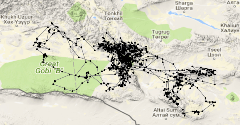
Figure 1: Relocations and trajectories of the Mongolian wolf Zimzik on Google Maps.

2 Statistical analysis of positional data

The statistical procedures to estimate home ranges are of a descriptive and nonparametric nature. They either estimate the home range directly, using geometric-type procedures, or they estimate first the utilization density and then compute the 95% level set of the density estimator. The earliest estimation techniques were based on scarce location data, which were assumed to be independent. However, the high-frequency observation in current tracking samples demands incorporating time dependence in the analysis of positional data. To distinguish between these two setups, in Subsection 2.1 we review the simpler home range estimators proposed under the independence assumption, and in Subsection 2.2 we introduce the more recent proposals dealing with time-dependent locations.

2.1 Assuming location data are independent

In this subsection we denote the animal relocations by $\mathbf{x}_{1},\ldots,\mathbf{x}_{n}$ and we assume they are independent realizations of a random vector $\mathbf{X}$ taking values in $\mathbb{R}^{2}$. In this setup, we begin by introducing global methods for home range estimation. The term “global” refers to the fact that each of such procedures is applied to the whole data set at once. In contrast, later we focus on the so-called localized methods, which stem from the former by applying a particular global method to each of the subsets of a suitably chosen partition of the data and then gathering up all the local pieces thus obtained.

2.1.1 Global methods

Minimum convex polygon (MCP) or convex hull

The convex hull of a sample of points is the minimum convex set enclosing them all, yielding a polygon connecting the outermost points in the sample and all whose inner angles are less than 180^∘. This is the simplest method for constructing home ranges and computing their areas and it has been widely employed for a long time, even until recently.

A variant of the MCP home range estimator is obtained by removing the proportion $\alpha$ of the sample points farthest from the sample centroid. More generally, Bath et al. (2006) compare the MCP home range after applying different criteria to “peel” individual observations from the sample of locations: they remove points farthest from the centroid or from the harmonic mean or those with a great influence on the area of the home range.

References using the minimum convex polygon (alone or in comparison with other methods) to estimate the home range of an individual are very abundant. Let us just mention a few: Mohr (1947), Odum and Kuenzler (1955), Worton (1987), Carey et al. (1990), Harris et al. (1990), Pavey et al. (2003), List and Macdonald (2003), Nilsen et al. (2008), Signer et al. (2015).

Obviously, the convexity restriction has serious drawbacks, among them home range overestimation, as illustrated in Figure 2, showing the MCP of Zimzik locations. The MCP was computed using the R package adehabitatHR (Calenge 2006). This home range does not adapt to the mountainous territory to which this wolf usually circunscribed its movements. To overcome this drawback, Harvey and Barbour (1965) proposed the minimum area method (also called by Kenward et al. 2001 the concave polygon). First, they computed the range length, the distance between the two locations furthest apart. Then, one outermost point (that is, in the boundary of the MCP) is connected with the next outermost one lying inside a ball of radius one quarter of the range length. The resulting minimum area home range is not necessarily convex and adapted better to the underlying sample shape.

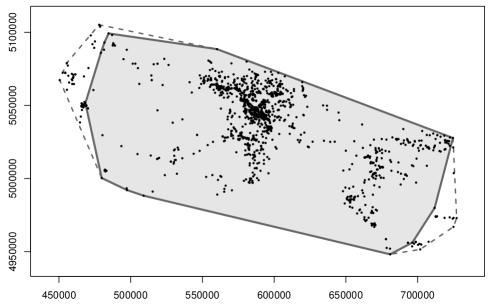
Figure 2: Minimum convex polygons for Zimzik location data: the MCP containing 95% of sample points is colored in grey. The dashed lines correspond to the MCP of the whole sample.

$\alpha$-convex hull

In the Computational Geometry literature, the notion of $\alpha$-convexity (first employed by Perkal 1956) is introduced as a generalized convexity concept, in order to relax the assumption of convexity, which can be very restrictive in practice. This is especially true in the problem of home range estimation, as illustrated above.

Rodríguez-Casal (2007) introduced the $\alpha$-convex hull of a sample of points and studied its convergence properties. Defined in simple terms, the $\alpha$-convex hull is the intersection of the complements of all the open balls of radius $\alpha$ which do not contain any sample points. Figure 3 shows the $\alpha$-convex hull of the observed Zimzik locations, with a value of $\alpha=18000$, computed using the R package alphahull (Pateiro-López and Rodríguez-Casal, 2016) after removing 5% of the data points farthest from the data centroid (see also Pateiro-López and Rodríguez-Casal, 2010).

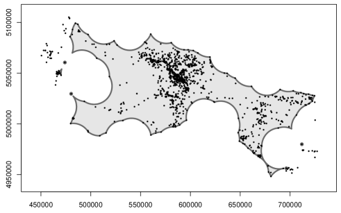
Figure 3: $\alpha$-convex hull estimation of the home range for Zimzik locations.

The boundary of this home range estimator clearly shows the arcs of some of the balls of radius $\alpha$ that form the complement of the estimator. The improvement over the convex hull is clearly noticeable, since the $\alpha$-convex hull does not contain some of the large portions of never-visited terrain that the convex hull enclosed.

The radius $\alpha$ controls the regularity of the resulting estimator: large values of $\alpha$ make the $\alpha$-convex hull very similar to the ordinary convex hull, and small values yield a quite fragmented home range estimator. The suggested value of $\alpha=18000$ was chosen here by visual inspection, but a recent research study proposes an automatic, data-based choice of this parameter (see Rodríguez-Casal and Saavedra-Nieves, 2016).

Let us point out that there are other existing home-range estimation techniques that receive a similar name to “$\alpha$-convex hull”, despite they refer to a completely different concept. To avoid confusion, it is worth mentioning the procedure of Burgman and Fox (2003), called $\alpha$-hull, which simply consists in obtaining the Delaunay triangulation of the data points and eliminating those line segments longer than a multiple $\alpha$ of the average line length. Although this latter $\alpha$-hull was initially introduced to estimate a species range, it has also been used for home range estimation (see, e.g., Foley et al. 2014).

In fact, Burgman and Fox’s $\alpha$-hull is closer to another related object in the Computational Geometry literature: the $\alpha$-shape of the data points. This is another generalization of the convex hull, defined as the polygon whose edges are those segments connecting two data points if there is an open ball of radius $\alpha$ having those two data points in its boundary and no other data point in its interior (Edelsbrunner et al., 1983). The $\alpha$-shape corresponding to Zimzik locations, computed with the R package alphahull, is depicted in Figure 4, for the same value of $\alpha=18000$ as before and after removing the 5% of the data points farthest from the data centroid. Its appearance is very similar to the $\alpha$-convex hull in Figure 3, with the notable difference that its boundary is formed by straight lines, instead of circular arcs.

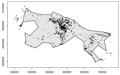
Figure 4: $\alpha$-shape estimation of the home range for Zimzik locations.

Still other recent generalizations of the convex hull are available for independent relocations, as for instance the cone-convex hull of Cholaquidis et al. (2014). In the case of dependent locations, Cholaquidis et al. (2016) propose to estimate the home range by the $\alpha$-convex hull of the trajectory or by the reflected Brownian motion (RBM) sausage (the outer parallel set of the trajectory). Here we will not explore these many variants.

Harmonic mean home range

Dixon and Chapman (1980) define the areal sample moment of order -1 with respect to a point $\mathbf{x}\in\mathbb{R}^{2}$ as the harmonic mean of the distances of $\mathbf{x}$ to the observed locations:

$$\mbox{HM}(\mathbf{x})=\frac{1}{n^{-1}\sum_{i=1}^{n}\|\mathbf{x}-\mathbf{x}_{i}\|^{-1}},$$

where $\|\mathbf{x}-\mathbf{x}_{i}\|$ is the Euclidean distance between $\mathbf{x}$ and $\mathbf{x}_{i}$. Then, as pointed out in Worton (1989), $\mbox{HM}(\mathbf{x})^{-1}$ can be considered as a kernel-type estimator of the UD, so that the harmonic mean home range is a level set of $\mbox{HM}^{-1}$ containing 95% of the locations. In fact, Devroye and Krzyżak (1999) showed that $\mbox{HM}(\mathbf{x})^{-1}$ is not a consistent estimator of the density, although this flaw is easily amended after a simple normalization, which consists of dividing $\mbox{HM}(\mathbf{x})^{-1}$ by $V_{d}\log n$, where $V_{d}$ is the volume of the unit ball in $\mathbb{R}^{d}$. In such form, it is called Hilbert kernel density estimate. In any case, note that the 95% level set is unaffected by that normalization. We display in Figure 5 the resulting home range, which obviously shares many of the drawbacks of the MCP.

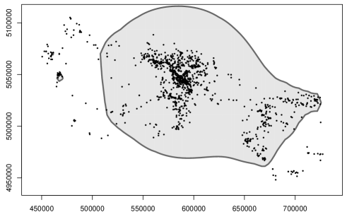
Figure 5: Harmonic mean home range for the wolf data.

Kernel density estimation (KDE)

Let us recall that $f$ denotes the utilization density. The home range of an animal is frequently defined as the level set $\{f\geq c\}$ of the utilization density attaining a 95% probability content, that is, the level set associated to the level $c=c_{0.05}$ such that

$$0.95=\int_{\{f\geq c_{0.05}\}}f(\mathbf{x})\,d\mathbf{x}.$$

Thus, a plug-in estimator of the home range is the analogous level set $\{\hat{f}\geq\hat{c}_{0.05}\}$ of an estimator $\hat{f}$ of $f$, where

$$0.95=\int_{\{\hat{f}\geq\hat{c}_{0.05}\}}\hat{f}(\mathbf{x})\,d\mathbf{x}.$$

The first proposals along these lines assumed a bivariate normal model for the UD (Calhoun and Casby 1958). Still in a parametric setting, Don and Rennolls (1983) used a mixture of normal densities to estimate $f$. However, noting that such parametric models were usually inappropriate, in a seminal paper Worton (1989) introduced kernel density estimators as a natural nonparametric approach in home range procedures.

The general expression of a kernel density estimator is

$$\hat{f}(\mathbf{x})=\frac{1}{n}\sum_{i=1}^{n}K_{\mathbf{H}}(\mathbf{x}-\mathbf{x}_{i}),$$ (1)

where $K:\mathbb{R}^{2}\to[0,\infty)$ is the kernel function (in this case, a probability density in $\mathbb{R}^{2}$), $\mathbf{H}=(h_{ij})$ is a symmetric, positive-definite $2\times 2$ bandwidth matrix, and the scaling notation $K_{\mathbf{H}}(\mathbf{x}):=|\mathbf{H}|^{-1/2}K(\mathbf{H}^{-1/2}\mathbf{x})$ has been used, with $\mathbf{H}^{-1/2}$ standing for the inverse of the matrix square root of $\mathbf{H}$.

It is well known that the choice of the kernel $K$ has little effect on the accuracy of the estimator $\hat{f}$, compared to that of the bandwidth $\mathbf{H}$. Worton (1989) chose a constrained bandwidth matrix $h^{2}\mathbf{I}$ (where $\mathbf{I}$ denotes the identity matrix) depending on a single smoothing parameter $h>0$, which was proposed to be selected either via the “ad hoc” method (i.e., optimal for the Gaussian distribution) or via least-squares cross-validation. Worton (1989) additionally considered an adaptive KDE, that is, a kernel-type estimator where the bandwidth is allowed to vary from one observation $\mathbf{x}_{i}$ to the other.

The KDE home range for the wolf data is displayed in Figure 6 for the one-dimensional ad hoc bandwidth $h=12269.09$ (as computed using package adehabitatHR) and the bidimensional unconstrained plug-in bandwidth matrix

$$\mathbf{H}=\left(\begin{array}[]{rr}23727441&-9074807\\ -9074807&10663700\end{array}\right)$$ (2)

of Chacón and Duong (2010), obtained with the package ks (Duong 2018). It is worth mentioning that, due to the very large values of the UTM coordinates, it was necessary to pre-spherify the location data in order for the numerical routine to be able to perform the optimization correctly. This means that the data were pre-multiplied by ${\bf S}^{-1/2}$, the inverse of the square root of their sample variance matrix $\bf S$, so that the sample variance matrix of the transformed data became the identity matrix. A plug-in bandwidth was obtained from these sphered data and was then scaled back by pre- and post-multiplying it by the $\bf S$ to finally obtain the above plug-in matrix for the original data (see Duong and Hazelton, 2003, Section 4).

As already noted by Bauder et al. (2015), the use of this unconstrained plug-in bandwidth matrix outperforms the single smoothing parameter approaches. The selected plug-in bandwidth matrix above suggests that, for this data set, it is advisable to use individual kernels with correlation coefficient $-0.571$, hence having their mass obliquely oriented, and not parallel to the coordinate axes as it happens when a diagonal or a single-parameter bandwidth is employed.

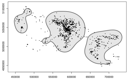
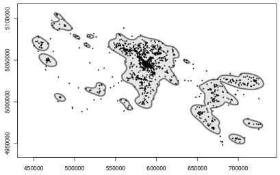
(a)	(b)

Figure 6: KDE home ranges for Zimzik data using (a) the one-dimensional ad hoc bandwidth $h$ and (b) the unconstrained plug-in bandwidth matrix $\mathbf{H}$.

Moreover, these UD estimators clearly reveal that just trimming points furthest away from the data centroid to obtain a region containing 95% of the data points might not be a good idea, since those points may not necessarily correspond to locations within low density zones.

Since its introduction, the use of the KDE home range has become widespread and a great deal of publications make use of it, even if the density estimator given in (1) is originally thought for independent observations (see Subsection 2.2). To cite a few case studies using this KDE home range, Bertrand et al. (1996), Kie and Boroski (1996), Girard et al. (2002), Hemson et al. (2005), Berger and Gese (2007), Pellerin et al. (2008), Jacques et al. (2009). Seaman and Powell (1996) and Seaman et al. (1999) analyze the KDE home range performance via simulations. Matthiopoulos (2003) presents a modification of the KDE to incorporate additional information on the animal.

Another ingenious modification of the KDE of a home range, namely the permissible home range estimator (PHRE), is given by Tarjan and Tinker (2016). These authors transform the original geographical sighting coordinates into coordinates with respect to relevant landscape features influencing animal space use. A KDE is constructed on the new coordinates and, afterwards, the corresponding estimated UD is backtransformed to geographical coordinates. The PHRE makes full sense in the context considered by Tarjan and Tinker (2016), but it is not clear that, in general, relevant features for the animal can always give rise to a new coordinate system.

2.1.2 Localized methods

The previous global methods share the common feature that they employ the whole data set (or a slightly trimmed subsample) at once to construct the home range estimate, either by applying some geometric construction to the sample points (convex hull and its variants) or by previously obtaining an estimate of the utilization density from them and then computing the density level set with 95% probability content (kernel methods).

In contrast, localized methods proceed in three steps: first, a local neighbourhood of points is selected according to some criterion (pre-clustering, nearest neighbours, points lying on a certain ball); then, one of the previous global methods is applied only to the selected points to obtain a local home range estimate, and, finally, many of these local home ranges are gathered together by taking their union. This way, many variants can be considered, depending on two choices: the way in which local neighbourhoods are constructed and the global method applied to each of these neighbourhoods. Next we describe the most popular ones.

Local convex hull (LoCoH) or k-nearest neighbor convex hulls (k-NNCH)

This is a localized version of the MCP. For a fixed integer $k>0$, Getz and Wilmers (2004) construct the convex hull, $k$-NNCH_i, of each sample point $x_{i}$ and its $k-1$ nearest neighbors (NN) (with respect to the Euclidean metric, although other metrics could be employed). Then these hulls are ordered according to their area, from smallest to largest. The LoCoH home range estimate is the isopleth that results of progressively taking the union of the hulls from the smallest upwards, until a specific percentage (e.g., 95%) of sample points is included. Getz et al. (2007) extend the original LoCoH procedure (called $k$-LoCoH) to the $r$-LoCoH (where a fixed sphere of influence was used instead of the $k$ nearest neighbours) and to the $a$-LoCoH (the $a$ standing for adaptive sphere of influence). A detailed study of the theoretical properties and finite sample performance of the $r$-LoCoH can be found in Aaron and Bodart (2016).

The optimal choice of the number of neighbours, $k$, depends on the topological features of the home range. In particular, one possibility is to choose the minimal $k$ resulting in a prefixed genus (number of holes), as long as this information is known. If it is not, Getz and Wilmers (2004) suggest guessing the genus after inspection of the physical characteristics of the territory. Another possibility is to examine the areas of the isopleths as a function of the values of $k$ (see the documentation of the R package tlocoh, Lyons et al. 2018).

The idea of incorporating topological information on the estimator has been little explored in the home range estimation literature. However, it represents a very active area in statistical research recently, encompassing a variety of methodologies under the name of Topological Data Analysis, which are nicely reviewed in Wasserman (2018) and implemented in the R package TDA (Fasy et al., 2017). Undoubtedly, the application of these modern techniques to the field of home range estimation shows promise as a very interesting venue for further research.

In Figure 7 we display the LoCoH home range for Zimzik data and $k=35$ neighbours, obtained with tlocoh. It is clear that this procedure is far more flexible than the convex hull, although it retains the simplicity of the latter.

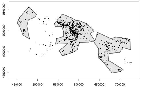
Figure 7: LoCoH isopleths with probability content 95% and $k=35$ neighbours for Zimzik locations.

Characteristic hull polygon (CHP)

As the LoCoH, the characteristic hull polygon (Downs and Horner 2009) is a union of convex sets and a generalization of the MCP. First, the Delaunay triangulation of the sample of locations is constructed. Then, the largest 5% of the triangles are removed, where the size of the triangle is measured by its perimeter. As Downs and Horner (2009) point out, it would be interesting that the proportion of triangles to remove should somehow depend on the actual shape of the real home range (for instance, this proportion should be 0 for convex domains).

The package adehabitatHR is the only one implementing the CHP in R, but it measures the size of the triangles by their area. We have modified the CharHull function from adehabitatHR to compute the perimeter of the Delaunay triangles and remove the 5% with largest boundary (see Figure 8). We see that this estimator resembles the LoCoH with $k=35$. As a home range, the CHP is unsatisfactory, since it includes several slivers corresponding to seldom visited locations, and, in particular, this produces two surprising holes that do not seem reasonable for the home range (by visual inspection of the sample shape and taking into account the geography of the terrain).

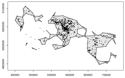
Figure 8: Characteristic hull polygon for Zimzik locations.

Single-linkage cluster

Kenward et al. (2001) proposed yet another localized variant of the MCP. The difference with the LoCoH lies in the way that local neighbourhoods are constructed. Their proposal starts from the nearest-neighbour distances between locations, these distances are clustered using single-linkage cluster analysis, aiming to minimize the mean joining distance and imposing a certain minimum cluster size. Once the locations are grouped in clusters, the convex hull (or the minimum area polygon) of each cluster is computed and the final home range is defined as the union of these polygons.

The single-linkage cluster home range of Zimzik locations data appears in Figure 9, produced using the package adehabitatHR. The method identified two larger clusters of locations, and several other smaller clusters, and obtained the final home range estimate by gathering together the convex hulls of each of the clusters. Nevertheless, it is noticeable that the convex hull does not seem to appropriately recover the shape of the main clusters, since the latter do not appear to be convex.

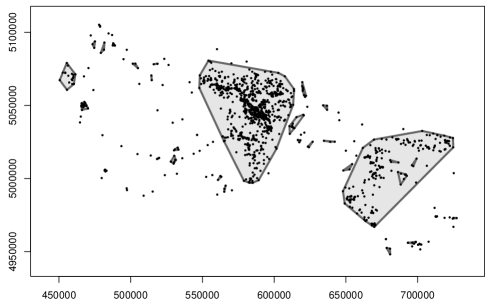
Figure 9: Single-linkage cluster home range estimation for Zimzik locations.

2.2 Incorporating time dependency

As noted in Subsection 1.2, the advent of GPS technologies to the animal tracking context has posed new interesting problems. The high frequency in the signal transmission originates stochastic dependence among locations which are close in time. This dependence should somehow be incorporated into the home range estimator, but it is also a source of information on the behavioural mechanisms of the animal.

In this subsection we review the proposals to incorporate the time dependency into the home range estimator. The sample including the observation times is denoted by $(t_{1},\mathbf{x}_{1}),\ldots,(t_{n},\mathbf{x}_{n})$, with $t_{1}<\ldots<t_{n}$. It should be stressed that for most studies the observation times are fixed by the researcher, so that they should not be treated as random.

We should also remind that static home range estimators are usually defined as a high probability contour of the utilization distribution. Most dynamic home range estimation methodologies seem to be also oriented towards this natural population goal, but some caution is required regarding recently proposed dynamic techniques, since some of them seem to lose track of the target that they intend to estimate.

2.2.1 Global methods

Time Geography Density Estimation (TGDE)

Time geography is a perspective of social geography introduced by Hägerstrand (1970). It analyzes human phenomena (transportation, socio-economic systems,…) in a geographic space taking into account the restrictions and trade-offs in human spatial behaviour imposed by individual activity schedules (see Miller 2005).

An important concept in time geography is the space-time prism, which bounds all possible space-time paths between two observed locations $\mathbf{x}_{i}$ and $\mathbf{x}_{i+1}$ at consecutive time points, taking into account the accessibility constraints of the individual (see Figure 10). The geo-ellipse $g_{i}$ or potential path area (PPA) of these two consecutive locations delineates in the geographic space all points that the individual can potentially reach during the time interval $[t_{i},t_{i+1}]$:

$$g_{i}=\{\mathbf{x}:\|\mathbf{x}-\mathbf{x}_{i}\|+\|\mathbf{x}-\mathbf{x}_{i+1}\|\leq(t_{i+1}-t_{i})v_{i}\},$$

where $v_{i}$ denotes the maximum velocity in the time interval.

Figure 10: Space-time prism and geoellipse $g_{i}$ corresponding to consecutive locations $\mathbf{x}_{i}$ and $\mathbf{x}_{i+1}$, observed at times $t_{i}$ and $t_{i+1}$ respectively.

Downs (2010) and Downs et al. (2011) propose to integrate KDE and time geography techniques by using the geo-ellipses derived from location pairs as surrogates for the KDE level sets. Downs (2010) claims that a drawback of KDE home range estimation is that it includes areas where the individual could not have been located, given the spatial and temporal constraints established by the observed locations and the maximum potential velocity. As an alternative, if the maximum interval velocities $v_{i}$ are all assumed to be equal to some global maximum velocity $v$, then the time-geographic density estimate at a point $\mathbf{x}$ is defined as

$$\hat{f}_{\mbox{\tiny TG}}(\mathbf{x})=\frac{1}{(n-1)[(t_{n}-t_{1})v]^{2}}\sum_{i=1}^{n-1}G\left(\frac{\|\mathbf{x}-\mathbf{x}_{i}\|+\|\mathbf{x}-\mathbf{x}_{i+1}\|}{(t_{i+1}-t_{i})v}\right),$$ (3)

where $G$ is a decreasing function playing the role of the kernel. Given that $G$ is maximal at zero, the individual summands of the estimator (3) assign the highest probability to the points along the straight path between two consecutively observed locations and spread out the remaining probability mass in ellipsoidal contours having the observed locations as their foci. The velocity $v$ plays the role of the smoothing parameter and, as such, it is reasonable to derive its value from the animal locations and their corresponding observation times (see Long and Nelson 2012). The TGDE home range is the 95% level set, $\{\hat{f}_{\mbox{\tiny TG}}\geq\hat{c}_{0.05}\}$, of the density estimate given in (3), where

$$0.95=\int_{\{\hat{f}_{\mbox{\tiny TG}}\geq\hat{c}_{0.05}\}}\hat{f}_{\mbox{\tiny TG}}(\mathbf{x})\,d\mathbf{x}.$$

In parallel, Long and Nelson (2012) defined the PPA home range as the union of the $n-1$ geo-ellipses obtained from all the pairs of consecutive locations in the sample:

$$\mbox{PPA}_{\mbox{\tiny HR}}=\bigcup_{i=1}^{n-1}g_{i},$$ (4)

with $v_{i}=v$, for all $i=1,\ldots,n-1$. The estimator (4) is a particular case of the TGDE home range $\{\hat{f}_{\mbox{\tiny TG}}\geq\hat{c}_{0.05}\}$ with a uniform kernel $G$.

Long and Nelson (2015) introduce the dynamic PPA home range (dynPPA), an adaptation of the PPA estimator to possibly different motion states. It is obtained by allowing the mobility parameter $v$ to change over time. In practice, these authors divide the trajectory of the animal in dynamic phases and obtain an estimator of $v$ in each of them.

The PPA home range and the TGDE are implemented in the R package wildlifeTG (Long 2017). In Figure 11 we show both home range estimators for the Zimzik locations data, where the function $G$ is Gaussian-like (i.e., proportional to $e^{-x^{2}/2}$) for the TGDE in (b). The PPA home range represents, in a sense, an upper bound of the home range since it clearly overestimates it by including all the locations that the animal could have reached if it had moved from each of the observed locations at a certain speed. TGDE is clearly the most satisfactory of the two, although it comprises many seldom visited areas.

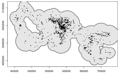
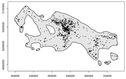
(a)	(b)

Figure 11: Home ranges for Zimzik data using (a) PPA and (b) TGDE with Gaussian kernel.

Kernel density estimation

There have been various attempts to generalize the kernel home range estimator to incorporate the time dependence between the observed locations. Nevertheless, there are two important issues that should be remarked: first, the definition of the kernel density estimator for dependent data is exactly the same as for independent data, and second, regarding the fundamental problem of bandwidth selection, the data can be treated as if they were independent, since the asymptotically optimal bandwidth for independent data is also optimal under quite general conditions of dependence, as shown in Hall et al. (1995). This means that, to design methods to estimate the utilization distribution density, we can proceed exactly the same as for independent data.

Keating and Cherry (2009) suggested a product kernel density estimator where time was incorporated as an extra variable to the two-dimensional location vector, thus yielding three-dimensional observations. This approach does not seem appropriate, since time is not a random variable whose frequency we want to analyze, as we noted at the beginning of Section 2.2.

In the context of estimating the active utilization distribution (describing space frequency use in the active moments of the animal), Benhamou and Cornelis (2010) developed the movement-based kernel density estimation (MKDE) method. MKDE consists in dividing each step or time interval $[t_{i},t_{i+1}]$ into several sub-steps, that is, adding new points at regular intervals on each step. Then KDE is carried out on the known and the interpolated relocations with a variable one-dimensional smoothing parameter $h_{i}(t)$. For each time interval $h_{i}$ is a smooth function of the time lapse from $t_{i}$ and to $t_{i+1}$, taking its smallest value $h_{\min}$ at the end points and the largest (at most $h_{\max}$) at the midpoint. A drawback of MKDE is that it depends, thus, on the choice of several parameters, such as $h_{\min}$, $h_{\max}$ and the length of the subintervals. For instance, using package adehabitatHR, in Figure 12 we have plotted the MKDE home ranges for two very different values of $h_{\min}$ but equal values of the rest of parameters: clearly, the choice of this smoothing parameter can substantially alter the resulting home range. Optimal simultaneous selection of all the parameters of MKDE with respect to some criterion is computationally unfeasible even for moderate sample sizes. A second concern regarding MKDE is that it is not clear whether the resulting home range differs substantially from the KDE based on the independence assumption.

There have been extensions to the original MKDE proposal. For instance, to incorporate knowledge of boundaries that the animal does not go through (rivers, cliffs, …), Benhamou and Cornelis (2010) suggest to reset to 0 beyond the boundary and reflect with respect to the boundary the resulting estimate of the utilization density. Also, Tracey et al. (2014) use the MKDE on 3-dimensional location data.

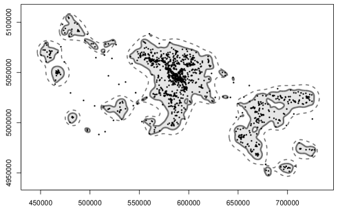
Figure 12: MKDE home range with $h_{\min}=1$ (continuous line) and $h_{\min}=5000$ (discontinuous).

Steiniger and Hunter (2013) propose the scaled line kernel home range estimator (SLKDE), which is similar to the MKDE of Benhamou and Cornelis (2010). Each line segment connecting two consecutive relocations, $\mathbf{x}_{i}$ and $\mathbf{x}_{i+1}$, is divided into subsegments and a KDE is constructed on each line segment based on observed and interpolated relocations. This estimator is called the raster $r_{i,i+1}$. Then all the rasters are pooled to construct an unnormalized estimator of the UD (it does not integrate to 1). The main difference with MKDE is that the smoothing parameter of the SLKDE is selected in such a way that it “inflates” the home range estimator on the observed relocations and thins it in the lines connecting them: the rasters have what Steiniger and Hunter (2013) call a “bone-like” shape. This procedure is not implemented in R.

Fleming et al. (2015) propose the autocorrelated kernel density estimator (AKDE). As usual, the probability density $f$ of the UD is estimated by a bivariate KDE $\hat{f}$ with a Gaussian kernel $K$ and an unconstrained smoothing parameter $\mathbf{H}$. As for the ad hoc bandwidth proposal of Worton (1989), the AKDE uses a bandwidth which is derived from the assumption of Gaussianity of the underlying distribution (which naturally leads to oversmoothing in most practical scenarios), with the only difference that instead of assuming that the location data are independent, they are supposed to be observations from a Gaussian stochastic process.

2.2.2 Localized methods

T-LoCoH

T-LoCoH (Lyons et al. 2013) generalizes the LoCoH home range to incorporate the observation times of the relocations. T-LoCoH incorporates the time associated to each location in two phases of the LoCoH algorithm: nearest neighbour selection and the ranking of hulls. First, the NN selection relies on the so-called time-scaled distance (TSD), which transforms the time coordinate into a third one of Euclidean space $\mathbb{R}^{3}$. Specifically, the TSD between two sample points, $(t_{i},\mathbf{x}_{i})$ and $(t_{j},\mathbf{x}_{j})$, is defined as

$$\mbox{TSD}_{ij}^{2}=\|\mathbf{x}_{i}-\mathbf{x}_{j}\|^{2}+s^{2}v_{\max}^{2}(t_{i}-t_{j})^{2},$$

where $s\geq 0$ is a scaling factor of the maximum theoretical velocity $v_{\max}$. Finally, to construct the isopleths, local hulls are sorted according to a hull metric, chosen to reflect the spatial or time information we might want to use. Dougherty et al. (2017) suggest a cross-validation procedure to select the tuning parameters $k$ and $s$ for the T-LoCoH.

Following the indications in Lyons et al. (2013), with the aid of the graphical procedures available in the package tlocoh, we have chosen the values of $s=0.05$ and $k=40$ as T-LoCoH parameters for Zimzik locations. The value of $v_{\max}$ was internally chosen by R. Figure 13 displays the resulting T-LoCoH home range. We notice that, in this case, there is not such a big difference between the LoCoH homerange (Figure 7) and the T-LoCoH one, probably due to the small value of the parameter $s$.

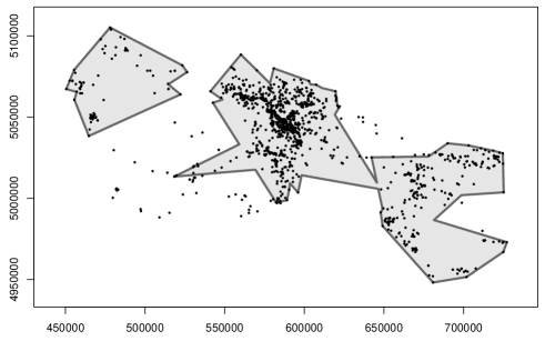
Figure 13: T-LoCoH isopleths for probability content 95%.

3 Ranking the home ranges

One of the key questions after computing several home range estimates based on the same positional data is how to select the most convincing or realistic one. In most case studies the biological expert chooses the soundest result according to previous information on the animal or its species. The possibility of making an automatised choice, based on objective statistical criteria, among a collection of home range estimates is, in a sense, still an open question.

There have been some attempts to compare home ranges according to different criteria. Here we briefly review the proposals valid for real data (methods only working for simulated samples are not considered). One possibility, especially if locations are treated as independent data, is to separate the sample into two subsamples of locations: a training sample to construct the home range estimator and a test sample to check its predictive accuracy. Approaches based on this idea have been used, for instance, in Kranstauber et al. (2012) and in Tarjan and Tinker (2016). Fleming et al. (2015) compare the areas of the home range estimates obtained with the complete sample and with the first half of the data (chronologically speaking). Long and Nelson (2015) compute the areas of different home range estimates. Kenward et al. (2001) study the relationship between the logarithm of the home range area and, for instance, environmental factors known to influence the animal behaviour (such as food availability or population density). Apart from the area, Steiniger and Hunter (2013) use shape complexity as given, for example, by holes and patches and the presence or not of corridors in the home range.

Cumming and Cornélis (2012) and Walter et al. (2015) compare home range estimates using the area-under-the-curve (AUC) corresponding to receiver operating characteristic (ROC) curves. The ROC curve (one for each HR) crucially depends on the choice of a certain raster containing all the home ranges. The curve is computed on the basis of the probability assigned by the UD to each cell in the raster and of the label indicating whether there is any sighting in the cell or not.

In this work we propose a new automatic way of choosing the “best fitting” home range among a collection, or at least a criterion for ranking them. The idea is to minimize a measure of the excess extension incurred by the home range as compared with the original locations, penalized by a measure of sample overfitting. The procedure is valid for any type of home range, regardless of the way it was constructed (for instance, estimating a utilization density or through geometric set estimation procedures).

To quantify the excess area of a certain home range with respect to the observed sample, we propose to intersect the Voronoi tessellation of the sample with that home range (see Figure 14). Then we sort the resulting (intersected) Voronoi cells according to their area (see Figure 15). We denote by $S_{(i)}$ the area of the $i$-th largest cell after intersection with the home range. Observe that zones contained in the set estimator but never or seldom visited by the animal usually correspond to large (intersected) Voronoi cells. We take the area of the largest cells as a proxy for the measure of the home range “hollowness”. Specifically we have computed $S_{(1)}$, the area of the largest Voronoi cell, and $\sum_{i=1}^{10}S_{(i)}$, the area of the ten largest cells. Other approaches such as taking a fixed proportion of the cells (i.e., of the sample size) could be considered.

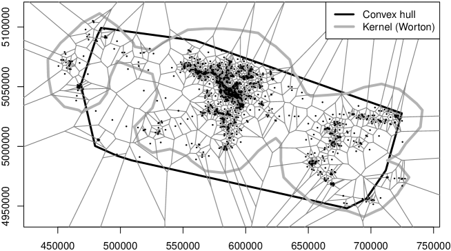
Figure 14: Voronoi tessellation of Zimzik relocations and two superimposed home ranges.

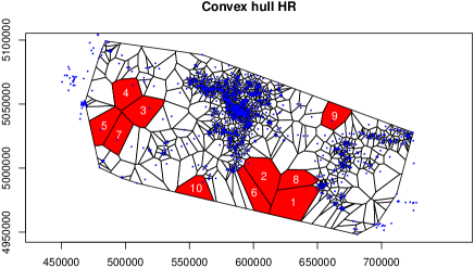
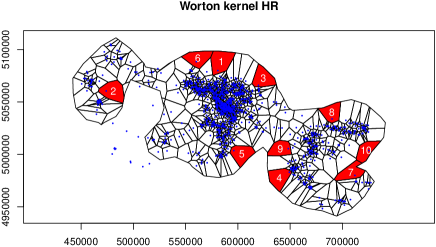
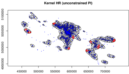
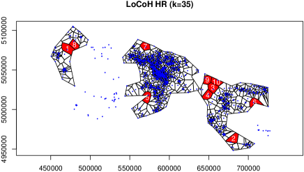
Figure 15: Intersection of Voronoi tessellation with some home ranges and highlight of the ten largest (intersected) cells sorted and numbered by area.

The home range area $A$, the maximum $S_{(1)}$ and the sum of the largest ten $\sum_{i=1}^{10}S_{(i)}$ areas of the Voronoi cells are displayed in Table 1 for a selection of home ranges based on Zimzik data. All areas are in $m^{2}$. The home ranges were selected for illustration purposes by their simplicity and/or reasonable graphical similitude to the original tracking data. The considered estimators are: the convex hull (containing only 95% of the sample points), the LoCoH with $k=35$ and $k=80$, the kernel estimator with the “ad hoc” smoothing parameter $h=12269.09$ used by Worton (1989) and with the unconstrained plug-in bandwidth matrix (2), the T-LoCoH with $k=40$ and $s=0.06$ and the MKDE with $h_{\min}=12000$ (a value slightly smaller than Worton’s bandwidth). We have also computed the area $B=\mbox{48,402,728,426}$ of the smallest bounding box containing all these home ranges. In Table 2 we display the ratios of $S_{(1)}$ and $\sum_{i=1}^{10}S_{(i)}$ over $B$ (in %), as a measure of how much the home range overestimates its target. As expected, for all these four measures the convex hull is the home range exhibiting the largest overestimation ratio, followed by the group formed by the LoCoH with $k=80$, the T-LoCoH, the kernel estimator with the “ad hoc” bandwidth $h$ and the MKDE. The kernel estimator with the plug-in bandwidth attains always the lowest overestimation ratio, followed by the LoCoH with $k=35$.

		Area of Voronoi cells
Home range	Total area $A$	$S_{(1)}$	$\sum_{i=1}^{10}S_{(i)}$
Convex hull	24,419,954,019	719,264,280	4,445,094,315
LoCoH ($k=35$)	10,851,131,941	148,388,790	1,078,176,739
LoCoH ($k=80$)	18,837,169,195	338,525,431	2,509,247,802
Kernel (Worton)	15,982,259,965	244,709,734	1,787,449,239
Kernel (plug-in)	8,083,494,038	53,206,494	455,072,754
T-LoCoH ($k=40$, $s=0.06$)	12,768,423,611	352,939,461	1,924,856,639
MKDE	22,944,329,048	330,576,812	2,638,851,646

Table 1: Home range area $A$, maximum area $S_{(1)}$ and area of largest ten $\sum_{i=1}^{10}S_{(i)}$ intersected Voronoi cells for some home ranges.

Home range	$S_{(1)}/B$	$\sum_{i=1}^{10}S_{(i)}/B$
Convex hull	1.49	9.18
LoCoH ($k=35$)	0.31	2.23
LoCoH ($k=80$)	0.70	5.18
Kernel (Worton)	0.51	3.69
Kernel (plug-in)	0.11	0.94
T-LoCoH ($k=40$, $s=0.06$)	0.73	3.98
MKDE	0.68	5.45

Table 2: Home range ratios (in %) of the areas of the intersected Voronoi cells over the area $B$ of an enclosing box.

HR estimator	$C$	$1/C$
Convex hull	0.7090	1.4104
LoCoH ($k=35$)	0.1510	6.6215
LoCoH ($k=80$)	0.4053	2.4674
Kernel (Worton)	0.2548	3.9251
Kernel (plug-in)	0.0723	13.8232
T-LoCoH ($k=40$)	0.1607	6.2229
MKDE	0.3101	3.2245

Table 3: Circularities for some home range estimators based on Zimzik relocations.

As a measure of how much a home range estimator overfits the underlying sample, we use shape descriptors (see, e.g., González and Woods 2008, Ch. 11). Specifically, since undersmoothing produces deep intrusions into the home range shape and consequently a perimeter increase, we have computed the shape circularity $C$, also called form factor, a simple descriptor taking values in (0,1]:

$$C=\frac{4\pi\,\mbox{area}}{\mbox{perimeter}^{2}}.$$

In particular, $C$ takes a value of 1 for a circular shape, but it is affected by the aspect ratio, so it can be close to 0 both for a flattened ellipse and a shape full of spikes. In Table 3 we display the circularity for the same home range estimators as in Table 1. The results are not surprising: the three estimators whose shape is more adapted to the sample (namely, LoCoH with $k=35$, the kernel estimator with plug-in bandwidth and the T-LoCoH) are the ones with lowest circularity ($<0.17$).

The overestimation ratios (in %), generically denoted by $R$, based on the Voronoi tessellation and the circularity $C$ are combined in a penalized criterion $R_{p}:=R+\lambda/C$, where $\lambda>0$ is a tuning parameter regulating the trade-off between the home range size and its goodness of fit to the locations. For Zimzik data, in Table 4 we reproduce the values of $R_{p}$ for all the home ranges and ratios $R=100\cdot S_{(1)}/B$ considered in the previous tables and for different choices of $\lambda$. Interestingly, we see that the LoCoH estimate with $k=80$ is the home range minimizing the penalized criterion in most occasions. In Table 5 we display the values of $R_{p}$ for $R=100\cdot\sum_{i=1}^{10}S_{(i)}/B$. Here it is the kernel home range, with the ad hoc choice of bandwidth, the one yielding better results, although the LoCoH with $k=35$ and $k=80$ has a similar performance. As a conclusion, we could say that the LoCoH (with a reasonable choice of $k$) and the kernel estimator proposed by Worton (1989) seem to be a reasonable and safe option in all circumstances. The MKDE is the time-dependent HR working best among those considered. Note, however, that the time-dependent estimators still have room for improvement since a more adequate choice of the smoothing parameters could diminish the criterion $R_{p}$.

		LoCoH		Kernel		T-LoCoH
	CH	$k=35$	$k=80$	Worton	plug-in	$k=40$	MKDE
$\lambda=0.01$	1.500	0.373	0.724	0.545	0.248	0.791	0.715
$\lambda=0.05$	1.557	0.638	0.823	0.702	0.801	1.040	0.844
$\lambda=0.1$	1.627	0.969	0.946	0.898	1.492	1.351	1.005
$\lambda=0.2$	1.768	1.631	1.193	1.291	2.875	1.974	1.328
$\lambda=0.3$	1.909	2.293	1.440	1.683	4.257	2.596	1.650
$\lambda=0.4$	2.050	2.955	1.686	2.076	5.639	3.218	1.973
$\lambda=0.5$	2.191	3.617	1.933	2.468	7.022	3.841	2.295

Table 4: $R_{p}$ values for $R=100\cdot S_{(1)}/B$.

		LoCoH		Kernel		T-LoCoH
	CH	$k=35$	$k=80$	Worton	plug-in	$k=40$	MKDE
$\lambda=0.5$	9.889	5.538	6.418	5.655	7.852	7.088	7.064
$\lambda=0.6$	10.030	6.200	6.665	6.048	9.234	7.710	7.387
$\lambda=0.7$	10.171	6.863	6.911	6.440	10.616	8.333	7.709
$\lambda=0.8$	10.312	7.525	7.158	6.833	11.999	8.955	8.031
$\lambda=0.9$	10.453	8.187	7.405	7.225	13.381	9.577	8.354
$\lambda=1$	10.594	8.849	7.651	7.618	14.763	10.200	8.676

Table 5: $R_{p}$ values for $R=100\cdot\sum_{i=1}^{10}S_{(i)}/B$.

Indeed, the new penalized criterion $R_{p}$ can be used as a tool for optimally choosing the parameters of the different home range estimators, by selecting the parameter value that minimises $R_{p}$. As an illustration, Figure 16 shows $R_{p}$ as a function of the bandwidth $h$ for the kernel home range estimator (left) and as a function of the number of neighbours $k$ for the LoCoH estimator (right), regarding the overestimation ratio $R=100\cdot\sum_{i=1}^{10}S_{(i)}/B$ and $\lambda=0.5$.

Figure 16: $R_{p}$ as a function of the bandwidth for the kernel home range estimator (left) and as a function of the number of neighbours for the LoCoH estimator (right).

The bandwidth that minimises $R_{p}$ for the kernel home range estimator is $h=7203.54$, and the resulting $R_{p}$ value is $4.987$, which is lower than the value obtained by any other method in Table 5 (for $\lambda=0.5$). The corresponding home range, shown in Figure 17, clearly displays a compromise by presenting a small overestimation area while, at the same, avoiding sharp inlets into the location data shape. Analogously, the number of neighbours that minimises $R_{p}$ for the LoCoH estimator is $k=65$, resulting in an $R_{p}$ value of 5.223, which is also lower than for any other method in Table 5, but still a bit higher than for the kernel estimator, meaning that in this situation the kernel home range attains a better balance between overestimation and too closely following the data locations. In any case, the LoCoH home range with this optimal value of $k$ is shown in Figure 18.

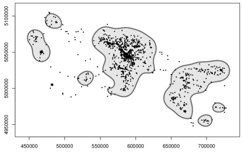
Figure 17: Kernel home range estimator for the Zimzik locations using the optimal $h=7203.54$ for $\lambda=0.5$.

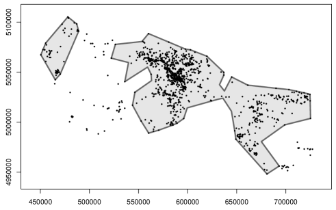
Figure 18: LoCoH home range estimator for the Zimzik locations using the optimal value of $k=65$ for $\lambda=0.5$.

4 Discussion

In this work, as a first aim, we have reviewed all the proposals in statistical home range estimation, up to the current state of the art. Assuming that location data are independent, the best global estimation procedure appears to be the kernel home range with an unconstrained bandwidth matrix and the localized method performing best is the LoCoH. Among the scarce methods taking into account the time dependence of the observed locations, the most suitable ones are actually adaptations to this context of the kernel and the LoCoH procedures, namely the MKDE and the T-LoCoH respectively. These two procedures depend on tuning parameters whose optimal choice has to be further investigated.

As a second objective, a natural consequence of this revision, we have proposed a general procedure to select the most appropriate home range among a collection of them based on the same set of relocations. The selection is performed via an index measuring the excess extension of the home range with respect to the relocations, penalized by the shape circularity to prevent over-fitting to the sample. When computing this penalization criterion on several home ranges based on the same real data set, the kernel and the LoCoH home ranges are the ones optimizing it. Further, optimization of the penalized selection index has led to a good-performing, natural choice of the tuning parameters in these home range estimators.