Neutrino Oscillations in Dark Backgrounds
Abstract
We examine scenarios in which a dark sector (dark matter, dark radiation, or dark energy) couples to the active neutrinos. For light and weakly-coupled exotic sectors we find that scalar, vector, or tensor dark backgrounds may appreciably impact neutrino propagation while remaining practically invisible to all other phenomenological probes. The dark medium may induce small departures from the Standard Model predictions or even offer an alternative explanation of neutrino oscillations. While the propagation of neutrinos is affected in all experiments, atmospheric data currently represent the most promising probe of the new physics scale. We quantify the future sensitivity of the ORCA detector of KM3NeT and the IceCube experiment and find that all exotic effects can be constrained at the level of a few percent of the Earth matter potential, with couplings mediating -neutrino transitions being most constrained. Long baseline experiments like DUNE may provide additional complementary information on the scale of the dark sector.
I Introduction
There are two indisputable signs of physics beyond the Standard Model (SM). The necessity to accommodate neutrino oscillation data points to either a new mass scale, say the seesaw scale, or new light degrees of freedom, i.e. right-handed neutrinos. The second reason why the SM is incomplete is the experimental evidence of a dark world, which we commonly refer to as dark matter and dark energy, that has been found to permeate our galaxy and more generally the whole visible Universe.
For what we currently know, it may well be that the above two puzzles have a common physical origin. This exciting possibility may be motivated by the apparent similarity in magnitude of the two effects, which both appear to be of order . Next, there is a question of opportunity. The laws of Nature tell us there are only a handful of ways in which the dark sector can couple to our world without spoiling the tremendous success of the SM. One such option is to make use of the neutrino portal, 111By neutrino portal we mean a coupling to the gauge-singlet combination , with the SM Higgs and the lepton doublets. Together with the other two portals — (Higgs portal) and the hyper-charge field strength (kinetic mixing portal) — they represent the SM-singlets with lowest dimensionality. Dark sectors with a neutral fermion, scalars, or vector bosons, respectively, naturally couple to these operators. that generally results in the introduction of exotic couplings between the active neutrinos and the dark world.
The existence of exotic couplings between active neutrinos and dark matter, dark energy or dark radiation, is expected to have indirect astrophysical as well as cosmological consequences and, if we are lucky enough, even direct signatures at colliders and dark matter experiments. Unfortunately, however, the absence of any clear indication as to where the new physics is hiding is suggestive that the latter is in fact too heavy to be directly accessible or possibly light but too weakly coupled to the SM. If this is indeed the case, then, is there any hope we will ever be able to directly access it? In this paper we suggest to use neutrino oscillations as a complementary probe of light, weakly-coupled dark scenarios coupled to us via the neutrino portal.
The coherent propagation of neutrinos in ordinary matter can amplify the otherwise small effects of the SM neutrino couplings to quarks and electrons Wolfenstein:1977ue Mikheev:1986gs . In a similar way, neutrinos propagating in the Cosmo may be affected by hypothetical tiny couplings to the dark medium that surrounds us. What makes neutrino oscillation experiments unique compared to other probes of dark sectors, is their ability to exploit this coherent enhancement to probe secluded sectors that are extremely weakly-coupled and otherwise invisible Capozzi:2017auw . This feature of oscillation experiments becomes immediately obvious once we recall that the strength of the neutrino interactions to ordinary matter at low momentum transfers is controlled by the Fermi scale , and realize that the latter quantity is actually a measure of the electroweak mass scale, and not of the electroweak coupling. In a world with a weak coupling smaller than ours by many orders of magnitude, the Fermi scale would still look the same to a physicist studying neutrino physics at momentum transfers . Neutrino oscillation experiments take advantage of the forward scattering with the medium, in which and the boson mass only enters via . The same argument generalizes to scenarios of physics beyond the SM: given a dark energy density , associated to dark matter or dark radiation or dark energy, neutrino forward scattering through this medium is sensitive to the combination , with a “dark Fermi constant” (we will see this in explicit models below). Secluded sectors with tiny couplings , that are not visible to experiments looking for processes that require sizable momentum transferred, can thus be probed in oscillation experiments if the mass scale characterizing the latter, , is small enough to compensate for the tiny density GeVcm3. Small dark scales appear in fact very reasonable, given that our current knowledge suggests that dark matter can be as light as eV whereas the dark energy might be associated to fields with masses less than eV.
In this paper we look at the signatures of neutrino propagation in a dark medium. In Section II we describe how the “effective Hamiltonian” relevant to neutrino oscillations is affected by interactions with general dark backgrounds. The outcome of this analysis, eq. (6), agrees with that obtained by earlier references, but we believe our derivation can provide useful to the reader intended to generalize the result including higher derivative interactions and other subleading effects. The exotic interactions are assumed to induce small corrections to the oscillation pattern characterizing the standard paradigm with three massive neutrinos. Yet, we will see in Section II.1 that a dark ether with certain key properties might actually mimic the effect of neutrino masses and thus represent a leading order effect. In such scenarios, neutrino oscillations themselves, as well as the relation , may be interpreted as the very first signature of the exotic interactions.
Among all oscillation experiments, in Section III we identify atmospheric neutrinos as key probes of these scenarios and estimate the experimental reach of two experiments. We argue that atmospheric data are, and will be in the foreseen future, necessary to constrain the relevant quantity . We show how the dark backgrounds can be generated in realistic models in Section IV. After a brief review of the scenario proposed in Capozzi:2017auw , we analyze an alternative vector model and the possibility of a dark radiation background, or dark CMB. This section demonstrates that oscillation experiments are unique probes of weakly-coupled dark sectors with masses of order keV or smaller.
Earlier work has constrained interactions between neutrinos and the dark world, see e.g. Capozzi:2017auw ; Fardon:2003eh ; Kaplan:2004dq ; Gu:2005eq ; Ando:2009ts ; Dvali:2011mn ; Ciuffoli:2011ji ; Berlin:2016woy ; Capozzi:2017auw ; Klop:2017dim ; Brdar:2017kbt ; Krnjaic:2017zlz ; Davoudiasl:2018hjw . However, our paper is unique in recognizing the pivotal role of neutrino oscillation experiments in probing light and weakly-coupled dark sectors, analyzing the effect of dipole interactions, and emphasizing the key role of atmospheric data. In our own Capozzi:2017auw we discussed a dark matter scenario capable of modifying solely solar data, but to achieve that feature some dark matter had to be captured in the sun, and this required additional interactions between dark and ordinary matter. Such additional interactions are not generic and not assumed here: in the present work no other interactions between the two sectors exist beyond those mediated by the neutrino portal.
II General backgrounds
Let us assume that, similarly to interactions with ordinary matter, the couplings of neutrinos to the exotic world are small enough that one can safely ignore the back-reaction of neutrinos on the dark medium. We will quantify this statement when we discuss explicit scenarios in Section IV. Under this hypothesis, we can describe the dark medium as a non-dynamical background.
The most general quadratic Lagrangian for a set of Weyl fermions interacting with an external background can be written as
with , , (the latter differs from other conventions by a factor of ) and are flavor indices. 222To avoid confusion, let us recall that Dirac neutrinos can be written as pairs of Majorana neutrinos (active and sterile), so our Lagrangian (II) and the results of this section are completely general and apply irrespective of whether the total lepton number is conserved or not. The numerical analysis in Section III will however assume Majorana neutrinos for definiteness. Finally, are assumed to be generated by exotic couplings to the dark world. In Section IV we will see how this might happen in explicit models.
With respect to the flavor indices , the mass is a complex symmetric matrix, the vector background is hermitian, and the tensor is a complex anti-symmetric matrix:
| (2) |
As we will see more explicitly below, the vector background mediates particle/particle and anti-particle/anti-particle transitions, whereas the tensor induces a particle/anti-particle mixing among different flavors. The latter may in general involve sterile components.
In general may depend on space-time position and contain derivatives acting on ; for example, a local vector background would look like . We will first comment on space-time dependent backgrounds in Section II.1 and then analyze in more detail constant backgrounds containing no derivatives starting from Section II.2.
II.1 Dark Backgrounds Faking Neutrino Masses?
Our first task here is to show that under special conditions dark backgrounds as in (II) can be the fundamental reason why neutrinos oscillate. This is easy to understand if we think of , since a constant is indistinguishable from a mass. 333The possibility of relating to a dark scalar background ( in (II)) was considered in earlier literature, see e.g. Fardon:2003eh and more recently in Refs. Davoudiasl:2018hjw ; DAmico:2018hgc . Space-time dependent can be distinguished from ordinary masses as will be discussed in Section IV.1. It is far less clear a priori that a vector and tensor background may accommodate neutrino oscillation data without the need of introducing neutrino masses, nor electroweak symmetry breaking. We will focus on , but similar considerations apply to .
Consider a background parametrized by a 4-vector that has a well-defined orientation within small domains of length size , but appears unpolarized at larger distances. More precisely, we assume that satisfies:
| (3) |
where represents an average over distances m. Indeed, experimental evidence of neutrino oscillations comes from local observations on scales of order hundreds of meters or larger. We therefore assume that Eqs. (3) are satisfied within microscopic domains of size larger than such scales (and of course smaller than astronomical distances, i.e. the macroscopic scales on which the energy density of the dark world is expected to vary). Our picture has an obvious analogy with ferromagnets: the vector represents the magnetization density and depends on the space-time position, the microscopic distance is set by the “magnetic domains”, whereas the macroscopic scale is the size of the magnet itself. Our magnet has vanishing total magnetization at distances .
Further assume the associated field has a flavor-violating coupling to the active neutrinos, as in eq. (II). By hermiticity of we can diagonalize the latter via a unitary transformation (that, in the basis in which the charged leptons are diagonal, represents the PMNS matrix). The dispersion relation for a given neutrino “ eigenstate” — where — reads (see eq.(8) with ), that is
where we neglected averages with 3 or more s and used (3). We see that for large as well as small 3 momenta the effect of such a dark ether is practically indistinguishable from an effective neutrino mass . To an observer that cannot resolve the polarization of , i.e. that cannot appreciate any departure from (3), oscillations of relativistic neutrinos can be induced by , and in particular proceed even in the absence of chiral symmetry breaking. This is somewhat analogous to the effect of a thermal mass at finite temperature.
It is now tempting to relate to the dark energy and perhaps justify , though at present we see no special reason why such a should be associated to dark energy rather than dark matter or dark radiation. The main model-building challenge is to find a dark vector field with the properties in (3). We will not attempt it here, however, and leave this task to future work. We simply note that, once an appropriate is found, obtaining the right coupling to neutrinos seems pretty straightfarward. For example, let us postulate there exists a scalar background whose gradient has inhomogenuities at small scales such that (3) is satisfied. We can then couple it to the lepton doublets via and effectively obtain , that can mimic neutrino oscillations if has spacial inhomogenuities of the right size. Corrections to the dispersion relation of the charged leptons are of order and therefore too small to be constrained by current data. Flavor-violating processes like do not represent a serious threat because sufficiently suppressed if is large enough.
It is interesting to consider the typical signatures of this scenario. From (II.1) we see that the effective mass is different at high and low energies: in the relativistic limit whereas in the non-relativistic limit . This latter aspect represents a characteristic signature that may be tested, for example, studying relic neutrinos or beta decay. Further tests could possibly come from extra-galactic neutrinos whose flavor ratio could be altered as they enter or exit the dark background.
In addition, there are other signatures one can consider. While the leading order effect described in (II.1) is practically indistinguishable from those of an actual neutrino mass, departures from the idealized limit (3) are characterized by corrections to the dispersion relation (II.1). These can be effectively parametrized by small and constant . Importantly, corrections to the standard paradigm of three massive neutrinos parametrized by small and constant are common to all our scenarios, whatever the UV origin of neutrino oscillations is. The rest of the paper is thus devoted to constrain those effects.
II.2 Constant dark backgrounds
In the remainder of the paper we will focus on backgrounds that are approximately constant within the length scales of interest, from a hundred meters to the earth diameter or longer. This approximation is justified because the distributions of dark matter and dark energy presumably vary on (extra-)galactic distances. And, as we have seen in Section II.1, even in scenarios with inhomogenuities at shorter distances, the most significant departure from the standard oscillation framework is still parametrized by the effect of (II) with approximately constant .
Furthermore, terms with additional derivatives acting on are usually subdominant and can be ignored. This is easy to understand in scenarios in which the interactions leading to (II) are mediated by heavy fields with masses of order a scale that is much larger than the typical neutrino energy . In those cases extra derivatives acting on would result in effects suppressed by powers of compared to those without derivatives. A similar conclusion generalizes to scenarios with light mediators. To be concrete, let us consider perturbative models — in which the dark backgrounds originate from the vacuum of spin fields . In these cases the higher order tensors necessary to build interactions with extra derivatives on , as for instance , must be obtained differentiating ; but these derivatives are typically suppressed under the hypothesis of approximate homogenuity of the dark medium.
These simple considerations motivate us to neglect any space-time dependence, as well as possible derivative interactions, in and focus on the more relevant case
| (5) |
Approximately constant vector and tensor backgrounds as in (5) signal a local violation of Lorentz invariance completely analogous to that implied by solids (made up of dark stuff, in our case). Also, CPT is locally broken by . Therefore the present paper can also be seen as an analysis of the leading effects of Lorentz and CPT violation. Our work has thus some overlap with Kostelecky:2003cr Kostelecky:2004hg (for a summary of the current constraints the reader may refer to Kostelecky:2008ts ). 444Many papers on this topic also include the effect of higher-derivative couplings such as . As argued above, however, these terms are expected to be subleading.
Let us now turn to a discussion of how neutrino oscillations are affected by the general Lagrangian (II) in the interesting cases described by (5).
II.2.1 The “Effective Hamiltonian”
In all instances of physical relevance, neutrino oscillations can be understood as the measure of the probability of a transition between stationary states with definite flavor, helicity, and energy traveling a spacial distance , see Lipkin:1995cb Stodolsky:1998tc (and Lipkin:1999nb for a more explicit discussion). The amplitude for such processes may be derived by calculating , with the operator associated to the 3-momentum along the flux and the distance between source and detector, i.e. the experimental baseline.
A careful derivation of is presented in Appendix A in the limit of small constant and ultra-relativistic neutrinos 555Because are Lorentz tensors, the term “small” is frame-dependent. Here we implicitly assume that are small with respect to an observer in the galactic or earth frames.. One can re-state our result (A) in a more familiar fashion. In the Schroedinger basis, and up to an unphysical phase, the propagation between source and detector may be described via , where is what is commonly referred to as effective “Hamiltonian” (though it is in fact an effective 3-momentum). Then, oscillations of properly normalized wave-packets with definite flavor and helicity are controlled by a matrix, with the number of Weyl neutrinos:
| (6) |
Here
with up to subleading corrections, , and is defined in eq.(A). The properties (2) imply that and , where complex conjugation and transposition are in the flavor indices and both matrices are allowed to be complex. In (II.2.1) we introduced the dark “electric” and “magnetic” fields and and used the relation . The expressions (II.2.1) make it manifest that in general do depend on the neutrino direction. In particular, while an isotropic vector background is possible if , the tensor interaction necessarily breaks rotational invariance by defining a preferred direction. 666In the ultra-relativistic regime the dipole is orthogonal to the direction of motion, , and therefore to the helicity. This is perhaps unfamiliar because a non-relativistic particle has a dipole moment proportional to its spin, . What the two regimes have in common, however, is that the dipole ceases to have physical effects when the external field is in the same direction as the particle’s spin. It is only when the polarization has a component orthogonal to the field that we see a “precession”, that here corresponds to a transition between different helicities.
Note that, at the leading order in the perturbations, eq. (6) coincides with the Hamiltonian found using a quantum mechanical approach in Kostelecky:2003cr . This is because under the assumption of constant backgrounds the momentum operator coincides with the one in the absence of the perturbations ( in Appendix A), and so small perturbations in the Hamiltonian effectively translate into a correction of the 3-momentum according to (20). In the presence of additional space-time derivatives or strongly varying backgrounds the two approaches would in general give different results, however.
It is possible to understand our result (6) without doing any actual computation. Indeed, it is important to appreciate that the necessity of having appropriate contractions of the flavor indices to render covariant uniquely determines where the various exotic backgrounds appear in (6). In particular the flavor symmetry implies that must be associated to particle/particle mixing and to anti-particle/anti-particle mixing and must therefore appear in the diagonal elements of (6). On the other hand, the only place where can show up is in the off-diagonal term, thus inducing particle/anti-particle transitions. This can be interpreted as the consequence of a flavor selection rule of (II) that forces to transform as , , and , where is an arbitrary rotation in neutrino flavor space. The need to properly contract the indices to form physical, re-phasing-invariant objects also selects the way appear in the oscillation probabilities, as we will see below.
The numerical factors in front of the various entries of (6) can be confirmed inspecting the eigenvalues of the Hamiltonian operator, that themselves follow from the neutrino dispersion relation:
| (8) |
Here all entries are understood as matrices in flavor space. The problem of finding solutions to (8) is considerably simplified when working at leading order in the perturbations. Within this approximation the mixed terms can be neglected, as can be seen employing the flavor selection rules mentioned above. This semplification implies that , where the dots contain three independent corrections proportional respectively to . We can now derive the leading corrections by solving three distinct dispersion relations, where are switched on one at a time. The case is standard and will not be described here. To study the effect of we switch off and neglect mixed terms involving multiplication of and . Eq. (8) is left invariant by the transformation . It follows that the two positive energy states have, at the order of interest, energies and . Within the conventions in the Fourier transform adopted in (8), particles (helicity ) have and anti-particles (helicity ) have consistently with (6). The vector enters differently in the energy of particles and anti-particles because it is odd under CPT. Finally, to derive the dispersion relation for we set and observe that can be diagonalized in flavor space. In that basis the determinant separates and, after some work, we find that for each flavor index the dispersion equation reads
| (9) |
where we introduced and in the second step of (9) the sum over the flavor index is understood. For each flavor there are two solutions , with . These coincide with those derived from (6). 777In the case of two flavors the relation can be readily used to show that , consistently with (A). The generalization to an arbitrary number of flavors follows. Hence we can conclude that (A) correctly reproduces the leading energy shift in the general case as well.
III Future constraints from Atmospheric Data
III.1 Why atmospheric data
The effective Hamiltonian (6) can be schematically written as the sum of the SM term and an exotic piece proportional to . It is useful to compare the potential of the main classes of neutrino oscillation data that can be used to set limits on : astrophysical, atmospheric, reactor, and solar.
Let us first assume that the exotic term leads to a small correction to the SM oscillation probability. This is equivalent to the statement that is small compared to the SM vacuum Hamiltonian. Assuming we have:
| (10) | |||||
| (11) |
where indicate the helicity. The oscillation length is controlled by the SM and is of course set by . The scaling laws in (10) (11) can be shown in complete generality, and are of course reproduced by the examples in Section C. Note that at short baselines only the off-diagonal entries in can be constrained by measurements, whereas long baseline experiments in principle have access to all elements because of the flavor transitions occurring in the SM.
The new physics term does depend on the neutrino direction but is otherwise approximately constant in energy, see (6). Hence, the relevance of the exotic term gets enhanced at large , when becomes less important, implying that experiments working at larger are sensitive to smaller . We thus expect atmospheric and astrophysical data to be more constraining than reactor and solar experiments.
This may be confirmed comparing the analysis of atmospheric neutrinos presented in Abe:2014wla with the sensitivity of the DUNE experiment, that should give a measure of the potential of long baseline experiments. The Super Kamiokande collaboration reports bounds of order GeV on transitions. 888With the same dataset, constraints of comparable order of magnitude may actually be obtained on the diagonal terms and as well, although these were not considered in that reference. The previous bound corresponds to an effect of order less than of the earth potential. The future sensitivity of DUNE on and NSI has been estimated in Coloma:2015kiu ; deGouvea:2015ndi , and can be translated into of the earth potential. This is in the ballpark of the current constraint from Super Kamiokande. Hence, existing atmospheric neutrino experiments already have a sensitivity comparable to the next generation of long baseline neutrino experiments, and we expect that future atmospheric data will only improve. 999For solar neutrinos the baseline is so large that the flux reaching the earth has completely lost its coherence and the new physics signature is encoded in an effective angle of order GeV, resulting on a deviation from the SM that is too small to be detected in current and future facilities. We thus conclude that solar data are not so very promising either. Note that the authors of Kostelecky:2003cr reach a different conclusion because implicitly assume that the new physics effect is controlled by . However, this is only true at short baselines.
The smaller SM background at high is the reason why astrophysical neutrinos are often suggested as the best probes for Lorentz Violating interactions, see e.g. Kostelecky:2013rv . However, above a certain critical energy, neutrino oscillation experiments have structural limitations that cannot be removed by reducing the systematic or experimental uncertainties. Indeed, in the regime the SM Hamiltonian is negligible, and the new physics actually dominates the transition:
| (12) |
This might seem a welcome property because one can efficiently isolate the effects of the new physics. However, (12) shows that the oscillation probability is now set by a “dark angle,” implying that the overall scale of cannot be constrained. In particular, the magnitude of the effect crucially depends on the relative size of the flavor-violating and flavor-conserving entries in , and can be significantly small if the diagonal elements of are sufficiently large. This represents an insurmountable limit for very energetic neutrinos. In fact, even in the presence of an ideal experimental precision and optimistically assuming the initial flavor content was known, one cannot set a robust constraint on the magnitude of employing only data with . One can clearly see this limitation in a recent IceCube analysis of GeV Aartsen:2017ibm , where atmospheric neutrino data alone cannot set an upper bound on unless further assumptions are made.
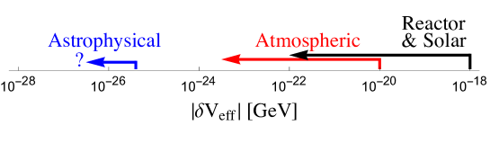
The main message here is that it is only for energies satisfying that we can, at least in principle, directly access the scale . The current situation is pictorially illustrated in Figure 1. Atmospheric data with GeV can be used to set a robust limit of order GeV. Reactors, accelerator and solar data have lower energies and are typically sensitive to larger exotic effects, see for instance Double-CHOOZ Abe:2012gw and MINOS Adamson:2012hp . Finally, astrophysical neutrinos have TeV and thus become fully effective only for GeV. Hence, in order to reliably take advantage of the very high energy domain we first need to robustly close the gap GeV GeV by improving our atmospheric analysis.
Motivated by these considerations, we next analyze in detail the potential reach of two atmospheric neutrino experiments: ORCA and the high-energy IceCube. The former is intended to provide a measure of the discovery potential of the low energy spectrum ( GeV), whereas the latter of the high energy tail ( GeV) of atmospheric data.
III.2 Analysis assumptions
In general, and the vector component of define a preferred direction in space, and force both to depend on the orientation of the neutrinos. A dedicated comparison among experiments would thus need to take into account the different orientations of the neutrino beams of the various facilities as well as seasonal variations. Since our paper is focussed on the prospects of current and future experiments, it would be impossible to include such effects properly. For this reason we will assume
| (13) |
are independent of throughout our analysis. This simplifying assumption is violated if a sizeable portions of the neutrino flux has significantly different directions, or if the duration of the experiment is long enough to appreciate seasonal effects. Still, because these latter conditions are quite special, we believe our assumption (13) is capable of capturing the most generic signatures of these scenarios. We will verify this claim a posteriori below.
Furthermore, a priori we have no reason to prefer a certain coupling over another. It is however not practically possible, nor particularly useful, to scan over all 15 parameters (13). We therefore decide to present our projections under the assumption that one complex coupling at a time is turned on. Besides simplicity, we believe this approach is defendable for the following reasons. First, phenomenologically viable scenarios have exotic potentials of a magnitude smaller than the SM effective potential. As a consequence, transition probabilities proportional to more powers of are suppressed compared to processes with a single insertion. Second, while correlations among the various entries in and/or are expected to be suppressed, there can still be non-trivial cancellations between the real and imaginary parts of a given which we find useful to show explicitly. This is emphasized in the example in Appendix C. We we do not anticipate that this feature applies to other s or to s, but for consistency (and as a check of our expectations) we will keep both real and imaginary parts of all couplings.
The reader should keep in mind that turning on more than one coupling can reduce sensitivity to a given coupling. This degeneracy has been previously seen in oscillation studies of NSI (e.g. Friedland:2005vy ; Liao:2016orc ) and persists for the and couplings introduced here.
III.3 Details on the numerical analysis
We report here the approach used for simulating both ORCA and IceCUBE experiments.
III.3.1 ORCA
The analysis of the prospective constraints of ORCA on and is performed analogously to what done in Capozzi:2017syc for the mass ordering. Here we only modify the calculation of the oscillation probability in order to accommodate the propagation of neutrinos in a generic background. For the sake of brevity we report below only the most important features of the analysis. Further details are found in Capozzi:2017syc .
ORCA Adrian-Martinez:2016fdl is a new low-energy neutrino telescope (part of the KM3NeT project) based on the Cherenkov detection technique in seawater, offshore from Toulon, France. The experiment is dedicated to studying atmospheric neutrinos of all flavors in the energy range [2,100] GeV. We focus here on upward-going neutrinos, i.e. with zenith angle [] where () represents the horizontal (vertical) direction.
The calculation of the event spectra in ORCA consists of three parts: production, propagation and detection. Concerning neutrino production we use the fluxes calculated in Honda:2015fha for the Frejus site, assuming no mountain overburden. Regarding neutrino propagation, we divide the Earth into five shells and in each we calculate the evolution operator up to the second order in the Magnus expansion Fogli:2012ua . Finally, all the ingredients relevant for simulating neutrino detection are taken from Adrian-Martinez:2016fdl , considering the configuration with 9 meters of vertical spacing between the optical modules. In particular, each neutrino event can be reconstructed either as a track or as a cascade, depending on its topology. We therefore divide the events according to these two categories.
We define as the number of simulated experimental data events of type (track, cascade) in the -th bin, where and represent the indices for energy and angular bins, respectively. are the current best fit values of the oscillation and systematic parameters, with an index labelling them. Note that we generate the mock experimental data assuming no non-standard effect in the propagation of neutrinos, i.e. . We define as the number of expected number events for a set of oscillation and systematic parameters (), in general different from their best fit, and either or . We calculate the marginalizing over systematic and oscillation parameters . This minimization is performed through the pull method Fogli:2002pt
| (14) |
where is the current uncertainty on oscillation and systematic parameters and represents an uncorrelated uncertainty in each bin. We adopt the default set of systematic uncertainties proposed in Capozzi:2017syc , i.e. including and a 1.5% residual uncertainty on the shape of the events distributions, which we parametrize as a quartic polynomial as in Capozzi:2017syc . All other sources of systematics with their correspondent uncertainties can be found in Capozzi:2017syc .
III.3.2 IceCUBE
IceCUBE is a neutrino telescope in the underground ice of the South Pole based on the Cherenkov detection technique. Despite being designed mainly for ultra-high energy neutrinos, i.e. those with energy greater than TeV, it performs also measurements of the atmospheric neutrino flux in the range [0.3,20] TeV.
The analysis method adopted for IceCube is similar to the one described for ORCA and summarized in Eq. 14. However, in this case we do not simulate the prospective mock data . Instead, in order to obtain any given exposure, we rescale the observed experimental data contained in a recent data release TheIceCube:2016oqi , 20145 muons collected in 343.7 days. The calculation of the expected number of events is performed by folding Monte-Carlo weigths, provided in TheIceCube:2016oqi , with the atmospheric neutrino flux and oscillation probability. The same data release contains information for the implementation of some systematic uncertainties. In particular, we consider a 2.5% error on the ratio in the atmospheric neutrino flux, 10% on the ratio , 40% on the total normalization and 5% on the cosmic ray spectral index. Regarding detection we are marginalizing over the optical modules efficiency and different ice models, where the first is a continuous variable and the second is discrete. Finally we use the Honda+Gaisser neutrino flux given in the data release associated with Ref. TheIceCube:2016oqi .
The data contained in TheIceCube:2016oqi seems to contain a statistical fluctuation which enhances the constraints on and (about a factor of 2) with respect to expectations for the same exposure. To obtain stronger constraints we therefore decided to rescale the observed distribution of events to obtain the mock data for a generic exposure, rather than simulating the data as done for our ORCA analysis.
III.4 Results
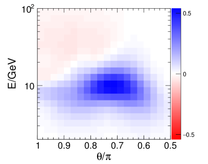
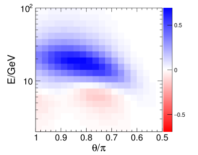
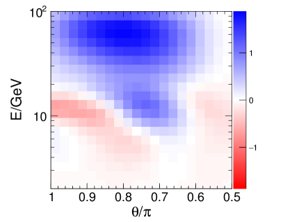
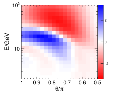
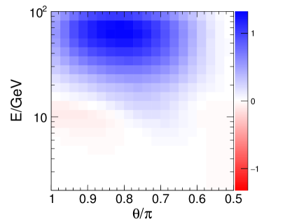
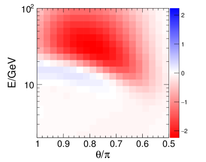
To get a physical sense of the types of modifications dark media can have on neutrino oscillations we display in Fig. 2 the deviations from the SM expectation as it varies with energy and zenith angle . The estimator of such a deviation is taken to be , the difference between number of events with and without divided by the square root of the SM prediction. As a representative sample we consider (top panel), GeV (middle panel), and (bottom panel).
Before discussing each case in turn, it is useful to make some introductory qualitative remarks. First, at high the flux is mostly composed of ; in track processes we mostly see neutrinos, whereas cascade events include all flavors. Second, high effects are dominated by new physics and maximized at longer paths. For this reason we expect the main SM deviations to peak towards . At low GeV the SM is sizable and the deviations are closer to , where the SM oscillation length peaks, .
These qualitative observations allow us to interpret the panels in Fig. 2. First consider the top panel of Fig. 2, showing the effect from . As in all cases with diagonal , this parameter requires interference with the SM in order to produce physical effects, resulting in a peak at relatively moderate energies. This is seen in both the track and cascade rates. By contrast, off-diagonal do not rely on the SM and their effect is usually maximized at large , when the SM contribution is suppressed. This is shown in the central and lower panels of Fig. 2 for and , respectively. Still, can also benefit from interference with the SM, unlike the case, thus explaining why the intermediate plots contain both low- and high-energy features in the distribution. The color coding is also consistent with physical expectations: tend to remove tracks (i.e. ) and generate cascades (i.e. in this case). Similar considerations apply to . Finally, we observe that all of the distributions exhibit rather broad deviations in zenith angle, . This justifies a posteriori our assumption that a more detailed analysis including directional dependence in the matter potential would not lead to very different distributions or sensitivities.
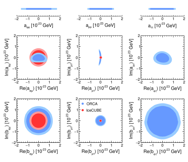
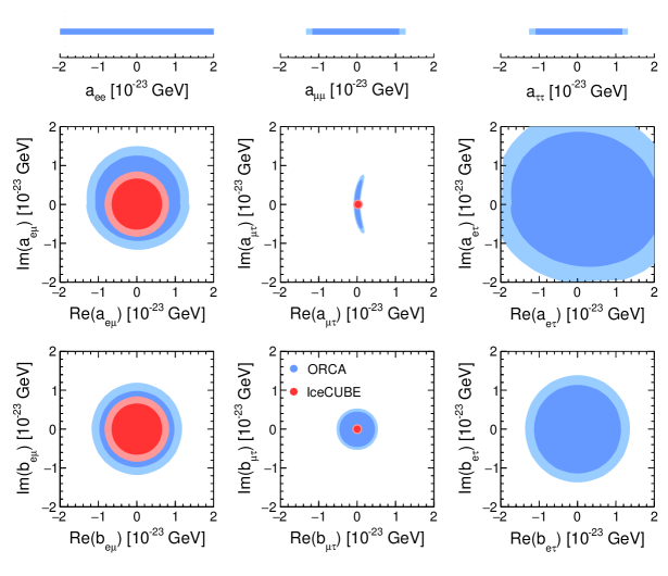
Let us now turn to the future sensitivity estimates we make for the IceCube and ORCA experiments displayed in Fig. 3 (for normal hierarchy, NH) and Fig. 4 (for inverted hierarchy, IH). On the upper panels we show the sensitivity to flavor diagonal couplings. As discussed above, since these couplings require interference with the SM to be observable our high-energy IceCube analysis is not relevant. Here the low-energy sensitivity of ORCA is therefore critical. Moreover, the sensitivity is roughly similar for all three neutrino flavors, with being somewhat more sensitive owing to the larger flux, large angle, and better flavor sensitivity in the track channel.
Regarding the flavor off-diagonal couplings of Figs. 3 and 4 we observe that is usually more constrained than whenever appears linearly in the oscillation probability (see (10) and (11)). On the other hand always appears quadratically, see also Appendix C. This latter point also explains why all allowed regions in are defined by circles of constant . A related feature that the figures reveal is that the IceCube constraints are symmetric in , whereas those from ORCA are not in general. This again follows from the fact that the SM contribution at the energies relevant to ORCA is not negligible. Consider the coupling for definiteness, for which an approximate expression for the oscillation probability is derived in Appendix C, see eq. (C.1). There it is seen explicitly that only the real part of appears linearly in (10), and that for moderate energies the contribution of the real and imaginary parts may partially cancel leading to non-trivial sensitivity in the complex plane. This explains the “banana” shaped contours in Figs. 3 and 4.
The main difference between Normal Hierarchy and Inverted Hierarchy is that in the latter case the SM neutrino conversions of neutrinos are less efficient, while the antineutrino transitions are enhanced but suffer from smaller statistics. Hence, the constraints on the parameters that take advantage of the SM (as emphasized above, this happens only at ORCA energies) are relaxed, see in Figs. 3 and 4. Also, the “banana” shape is reversed because changes sign.
In general we observe a very rich structure with both low and high energies contributing in a non-trivial way to event distributions (see the middle panel of Fig. 2). This richness leads to IceCube being stronger in some cases () and ORCA being stronger in the others (). It is also worth recalling that our IceCube analysis relies only on muon neutrinos, so that the transitions at IceCube are not probed.
IV Models
Now we turn our attention to realistic models with neutrino couplings to dark sector states. We will examine various implications of additional neutrino-DM interactions and provide a consistency check on the framework. We will see that in the present scenarios there are large regions of parameter space where neutrino oscillation modifications set far stronger limits than any other physical process.
Phenomenological considerations similar to the ones presented in this section have been previously presented in Capozzi:2017auw in an Asymmetric DM model. There it was emphasized that a very efficient way to generate effective couplings for active neutrinos — without spoiling the physics of the charged leptons — is via the mixing with exotic fermions that couple to the dark sector Capozzi:2017auw . For definiteness we will assume this mechanism is at work in all the models we discuss. We will not consider cosmological constraints on the sterile sector, however. These can be very constraining, but are in general model-dependent. To be on the safe side we will assume cosmology is standard because the active-sterile mixing started at very late stages of the Universe’s history Patwardhan:2014iha ; Vecchi:2016lty .
IV.1 Scalar
A correction to can only lead to observable effects if it possesses some space-time dependence. Otherwise, would be indistinguishable from a neutrino mass.
To realize a space-time varying we need a scalar dark field with a space-time dependent background. Consider scenarios in which is a classical field oscillating around the origin of field space with energy density . If some coupling to neutrinos (active or sterile) exists, say , one can obtain an effective space-time-varying mass of order
| (15) |
with the active/sterile mixing. Note that, consistently with the general scaling argument presented in the introduction, this has the structure with . This possibility has been considered recently in Berlin:2016woy ; Krnjaic:2017zlz ; Brdar:2017kbt . The authors find that such effect may result in observable variations in neutrino oscillations if is of the order of the local dark matter density, eV, and the oscillation frequency is not much larger nor smaller than years.
In concrete examples, however, the non-derivative couplings of must be very small. Otherwise, sizable couplings would generate large quantum corrections to the scalar potential, both at zero and finite temperature. The former should be minimized in order to avoid a large fine-tuning. This is often achieved assuming is an approximate Nambu-Goldstone boson, in which case with some large scale. With this expectation, however, neutrino experiments would be unable to detect any effect in the foreseen future. Yet, if we ignore the fine-tuning problem and allow , we still have to deal with large thermal effects that can dramatically impact the evolution of the scalar. For example, thermal corrections of order would prevent the scalar from behaving as cold dark matter until . Because we experimentally know that dark matter was already present at eV, one can derive — barring miraculous coincidences — a structural constraint eV that is stronger than the projected sensitivity of future neutrino experiments. may also be identified with a subdominant dark matter component or even radiation, but in these cases its density would be too small to have a sizable effect.
Our conclusion is that is basically indistinguishable from a constant mass term unless a large amount of fine-tuning is invoked. We will therefore focus on in the rest of the paper.
IV.2 Vector
In the following we consider the possibility of a dark . We focus on scenarios in which the latter is generated by a fundamental vector field, but the reader should keep in mind that is another interesting possibility.
IV.2.1 Model 1: Asymmetric Dark Matter Coupled to an Ultra-Light Vector
In a previous paper Capozzi:2017auw we discussed a simple realization of the vector scenario in which an asymmetric dark matter background with density sources a spontaneously broken dark vector field coupled to (sterile) neutrinos, thus generating
with the active/sterile mixing ( if a direct coupling between active neutrinos and the dark world exists), and the vector coupling and mass. In the second line of (IV.2.1) we estimated the magnitude of the current assuming it is due to a dark matter candidate of mass and matter density GeVcm3. Hence we find the scaling . Importantly, while weakly-coupled sectors cannot be directly probed otherwise, they can still show up in neutrino oscillation experiments if is large enough.
A quantitative discussion of the astrophysical and cosmological impact of this picture can be found in Capozzi:2017auw . In that work it was found that IceCube and SN1987A can place stringent bounds at low mediator masses by inducing a neutrino mean free path for scattering on the cosmic neutrino background. At larger mediator masses, , bounds on DM kinetic decoupling in the early universe from elastic scattering on the relativistic neutrinos become the most stringent non-oscillation bounds. All these become ineffective as decreases, however.
IV.2.2 Model 2: Ultra-Light Vector DM
An additional model for vectorial DM interactions with neutrinos was introduced in Brdar:2017kbt , as an extension of the model of vector DM sourced by inflation in Graham:2015rva . For definiteness, we assume that the only relevant couplings of the vector is to sterile neutrinos as in Capozzi:2017auw
| (17) |
where is the new gauge coupling of the theory. We leave both the mass scale of the steriles and their mixing angles with the active neutrinos unspecified. Note that unlike Brdar:2017kbt we do not explore gauged lepton number models but instead focus on models where the sterile sector is charged under the new gauge symmetry.
In this case it is the VEV of the vector, , that induces a matter potential
The potential now scales as , with .
Note that sizable effects in neutrino oscillations are obtained with an extremely small coupling . Because of this, all other constrains can be evaded, as emphasized in the introduction. Additional constraints here mainly come from: (1) dangerous early Universe processes which can equilibrate neutrinos and DM, (2) early Universe freeze-in Hall:2009bx of DM, and (3) present-day bounds on the neutrino mean free path from SN1987A Kolb:1987qy and IceCube Cherry:2014xra ; Cherry:2016jol . We find all of these to be many orders of magnitude weaker than the oscillation bounds. The details of these constraints are outlined in Appendix B.
IV.3 Tensor
Tensor couplings parametrized by are induced by dipole interactions with a dark gauge boson whose electric or magnetic fields are non-trivial. This interaction is expected to dominate over a possible background if the gauge symmetry associated to is unbroken. Indeed, gauge invariance may forbid a direct interaction between (active or sterile) neutrinos and , in which case would parametrize the leading effect.
Neutrino oscillations mediated by an electro-magnetic dipole moment were first studied in Cisneros:1970nq . Here we will allow the potential to be entirely due to dark forces. In practice, our tensor coupling parametrizes the interactions between neutrinos and a “Dark CMB”.
To estimate the size of , we imagine adding exotic neutrinos that mix with the active ones as in Capozzi:2017auw and have a Yukawa coupling with two particles charged under the dark radiation. This framework predicts
where we take the current Dark CMB density to be , whereas is the largest mass of the two mediators , and finally is the gauge coupling. Note that despite the rather small values of , the effective operator description remains valid in our oscillation setup up since the oscillation impact comes from scattering at negligible momentum transfer. In this case the dark background is again scaling as , though now .
Similarly to the vector models, we find that the most constraining non-oscillation data comes from SN1987A. Assuming negligible relic abundances for (which may have annihilated away into dark radiation), the neutrino flux is depleted via , where are active or sterile relic neutrinos. We estimate that the total cross section for the latter processes scales at most like . Requiring the mean-free paths for the neutrinos emerging from the supernova is long enough we find a rather weak bound on the coupling, . Again, oscillation experiments provide the dominant constraints in the weak-coupling, low-mass regime.
V Conclusions
Neutrinos acquire exotic interactions in many extensions of the Standard Model. The effect of non-standard couplings to ordinary matter has been investigated extensively in the literature, both in the context of oscillation experiments as well as colliders. These are usually very severely constrained by rare processes involving charged leptons and quarks. Here we considered the possibility that the new couplings involve a dark sector. Such a picture is far less constrained and neutrino experiments can play a pivotal role. In fact, the dark energy, dark matter, and possibly dark radiation that permeates the world around us might act as a medium affecting neutrino propagation in a non-trivial way while still being undetected otherwise: neutrino oscillation experiments represent a unique opportunity to detect light dark sectors interacting with our world via the neutrino portal.
Given our ignorance on the nature of dark sector physics we have considered the most general classes of backgrounds: scalar, vector (parametrized by a hermitian matrix ), and tensor (parametrized by an antisymmetric matrix ). Neutrino oscillations in the dark medium can be described via an effective “Hamiltonian” that we derived under the hypothesis that the exotic fields are nearly constant within the relevant space-time scales, and induce subdominant effects on top of ordinary neutrino oscillations. The true origin of the leading neutrino oscillations is not crucial to our numerical analysis, and may be due to ordinary masses or even the dark backgrounds themselves. While the statement that a dark scalar background can be responsible for neutrino oscillations comes hardly as a surprise, we showed that even vector and tensor backgrounds with anisotropies at small scales may in fact mimic vacuum oscillations without the need to invoke neutrino masses nor chiral symmetry breaking.
Neutrino forward scattering is affected by an effective potential that scales with appropriate powers of , where is a dark “Fermi scale” of the exotic sector and is the dark background energy density. Neutrino oscillation experiments are unique probes of scenarios with small and sizable , when all other probes become inefficient.
Models in which the dark background is generated by a density current have , as in the SM, whereas when the dark density is generated by the vacuum expectation value of bosonic fields one finds . In either case a determination of is necessary to extract useful information on the scale of the dark sector. We have argued that can only be constrained by experiments that have the ability to probe the energy range in which , with indicating the SM effective Hamiltonian. On the other hand, for too large energies the SM background becomes irrelevant () and we lose access to the magnitude of . For this reason atmospheric neutrinos turn out to be a necessary input for other, more energetic probes. To close the gap schematically shown in figure 1, a careful analysis of atmospheric data is necessary.
We analyzed the sensitivity of the ORCA detector and the IceCube experiment to dark backgrounds. We find that these experiments have impressive sensitivity, especially in the - sector, and an interesting complementary, with IceCube’s high-energy sensitivity setting the leading constraints on , , and and ORCA providing stronger bounds on , , , , , and .
The atmospheric neutrino flux we have focused on has important limitations however. A major drawback is the poor discrimination power, which inevitably impacts the sensitivity to the tensor interaction . Moreover, atmospheric neutrinos are mostly sensitive to muons, with transitions being only weakly constrained at present. Long-baseline experiments such as DUNE will therefore be crucial in the search of dark backgrounds . Based on the estimates made in Coloma:2015kiu ; deGouvea:2015ndi , for certain couplings DUNE may have sensitivity competitive with atmospheric data. The possibility of better discrimination may aid DUNE in improving the constraints especially on tensor backgrounds not considered in Coloma:2015kiu ; deGouvea:2015ndi .
Acknowledgments
IMS is very grateful to the University of South Dakota for support. F.C. acknowledges partial support by NSF Grant PHY-1404311 to J.F. Beacom, the Deutsche Forschungsgemeinschaft through Grant No. EXC 153 (Excellence Cluster ”Universe”), Grant No. SFB 1258 (Collaborative Research Center ”Neutrinos, Dark Matter, Messengers”) as well as by the European Union through Grant No. H2020-MSCA-ITN-2015/674896 (Innovative Training Network ”Elusives”). The work of LV is supported by the Swiss National Science Foundation under the Sinergia network CRSII2-160814.
Appendix A Derivation of (6)
We here aim to derive in the presence of small backgrounds , with the unperturbed mass. To proceed we make three simplifying assumptions, that are motivated in the text:
-
(1)
the do not violate space-time translations;
-
(2)
do no contain space-time derivatives acting on ;
-
(3)
can be interpreted as small perturbations.
With the first assumption, the full energy-momentum operator is conserved, and we are allowed to write . Here and in the following we denote by the 4-momentum operator in the absence of (but with a mass ). Then, defining — with the subscript indicating that this field satisfies the free field equations — we have .
Assumption (2) implies that and, together with , allows us to obtain the important result . For simplicity, since become essentially indistinguishable, we simply set in and forget about in the following. Note that a standard calculation tells us that in the ultra-relativistic regime , with a small correction. From this latter definition and the first two assumptions immediately follows that, for a given neutrino direction:
| (20) |
where represents the term induced by expressed in the interaction picture.
Finally, assumption (3) allows us to expand in the perturbations and obtain
While is time-independent, in general does depend on . However, the above form is very useful in practice because is straightforward to compute under the first two assumptions: we just need to calculate on a solution of the free field equations associated to .
We are now in a position to obtain our result (6). To introduce the notation that we will adopt in the following, we write in terms of the creation operators of neutrinos of a given helicity ( for particles and for anti-particles) and flavor index . Ignoring terms of , a standard calculation gives
The flavor indices have been suppressed for simplicity. The reader should interpret as matrices in flavor space. With our conventions, the operators carry helicity and flavor indices and generate 1-particle states . The creation/annihilation operators satisfy .
Because in (A) we are ignoring mixed terms involving products of , the free field used to determine can be taken to be a solution of the massless equation:
| (23) |
with and a complete set of spinors. They are functions of with negative and positive helicity, . Inserting (23) in we finally obtain:
Again, flavor indices have been suppressed for brevity. In obtaining (A) we used , the completeness relation , and defined . From the previous definition follows that satisfies , , . The latter polarization tensor was previously used in Kostelecky:2003cr .
Eq. (A) is the final result; from it one can obtain (6) observing that , with is defined in terms of (A) and (A). A few comments are in order. First, as mentioned at the beginning of this section, oscillation probabilities depend on the amplitudes , with initial and final states constructed via linear combinations of with the same energy (but in general different 3-momentum) and well-defined flavor and helicity quantum numbers. The factors of in (A) thus become immaterial phases and neutrino propagation is effectively controlled by .
Second, the operator depends explicitly on . However, this dependence disappears from the oscillation probabilities, consistently with (20). Indeed, the time dependence is relegated to the terms of (A). These have vanishing matrix elements with (that are linear combinations of ) and can be neglected in the study of neutrino oscillations.
Finally, note that the same procedure employed to derive (A) may be used to obtain a matter potential in the case of slightly varying backgrounds. The result would be the same as in (A) as long as the length scale within which the potentials vary is much longer than . In that case one can split the calculation in various regions of approximately constant backgrounds, where (A) holds. In particular, our result with reproduces the standard matter potential of Wolfenstein:1977ue Mikheev:1986gs .
Appendix B Constraints on the ultra-light vector dark matter model
Here we briefly summarize some of the bounds on the ultra-light vector dark matter model of Sec.IV.2.2, beyond neutrino oscillations. We will see that these are substantially weaker for sub-eV mediators.
Having set the scale of masses and couplings relevant for oscillation modifications in Eq. IV.2.2, let us turn to other potential phenomenological constraints. Despite the small DM masses in this setup, the vector DM produced from inflation is quite “cold” and thus does not spoil the successful predictions of standard CDM Graham:2015rva . This makes the introduction of the neutrino coupling potentially dangerous since these relativistic particles can inject energy into the cold DM population and heat it up, or produce a population of hot DM directly. Although one typically has to worry about the impact of late kinetic decoupling in “neutrinophilic DM” setups (see Capozzi:2017auw ), here the problem is more severe. In the present case it is required that DM- interactions never come into equilibrium. Let’s examine the potential problems from this.
The most dangerous processes that proceeds until late times is (inverse) decays of the sterile, . We estimate the rate of this decay in the early Universe to be, . As we approach the temperature two things happen: (1) the boost factor in front of disappears and (2) the sterile population is rapidly depleted. Crucially this processes must remain always out of equilibrium () to avoid producing a sizable abundance of hot DM from the decay products. Notice that is maximal around . Thus by requiring that at we conservatively obtain
| (25) |
for any value of kinematically accessible.
At higher processes like annihilation will dominate since . However we find that the bound obtained from such annihilation processes is always less stringent than Eq. (25). Notice that is in contrast with what was found in Huang:2017egl . This difference can be understood as follows. First, unlike Huang:2017egl , we are taking the vector to constitute the DM and not merely to be constrained by contributions to the relativistic energy density around MeV temperatures as in Huang:2017egl . Second since we are operating in the extremely small coupling regime the rate for annihilation processes () is extremely suppressed compared to inverse decays (). Lastly, note that in the eV regime the vector is stable while the sterile neutrino opens an additional path for thermalization, .
Next, consider the possibility that the sterile neutrino is absent at the relevant epochs in the early Universe. This could happen for example in models with heavy sterile neutrinos. Then integrating out the steriles the only impact of the vector is through an effective coupling to active neturinos, . Then annihilation can produce a hot population of ’s. Requiring the rate of this annihilation process to be sub-Hubble at CMB times implies, .
Now we turn to present-day bounds. A well known constraint on the properties of neutrino interactions comes from the observation of the neutrinos observed in 1987A. The detected from the supernova can be removed by scattering on background DM or neutrinos. We find that the neutrino background places the strongest constraints despite the larger DM density. This comes about because the -channel scattering via exchange is strongly enhanced at small-. Although a small momentum is exchanged, the scattering can “sterilize” the neutrino flavor content, Cherry:2014xra ; Cherry:2016jol .
To compute the optical depth for this process we include the possibility of local gravitational clustering of neutrinos in the Milky Way. This has been estimated to lead to clustered number densities above the smooth cosmic background Ringwald:2004np . Then the optical depth is , and we model the neutrino density along the line of sight as , where the first term is the MW contribution and the last term is the cosmic contribution (taking as a model of the MW matter density). Using we find that requiring the optical depth to be less than unity implies
| (26) |
We note that a similar process can modify the PeV astrophysical flux seen by IceCube. However the extremely small mediator masses produce larger effects in MeV supernova neutrinos. We note that in models where the sterile are heavy enough to be irrelevant at these scales, one can still obtain a SN1987A bound from the energy losses an incoming suffers from significant momentum-transfering collisions Kolb:1987qy .
Appendix C Effective Hamiltonian: Illustrative examples
It is instructive to discuss a few scenarios in which (6) can be studied analytically. We consider either or , since combinations of the two parameters always result in subleading effects.
C.1
Neglecting and the SM effective Hamiltonian has no entries and we are justified to consider the subset of the full 6 by 6 matrix (6):
| (27) |
where are real numbers defined by:
| (28) | |||||
whereas is obtained replacing in . The oscillation probability is immediately derived from
| (29) | |||||
and reads . For intermediate ,
and a partial cancellation between may take place. We see this correlation at play in our numerical results.
C.2
An analytic solution cannot be written in a simple form when also the SM effective hamiltonian is included. However, the analysis simplifies considerably at high energy, when we can approximately write
| (31) |
and one finds
| (32) | |||||
The flavor selection rules imply that neutrino/anti-neutrino transitions are proportional to and determine the form of the transition probability, . Neutrino/neutrino conversions are also possible, but the flavor selection rules now imply that the amplitude is controlled by , so : flavor conversions may happen only if two or more independent terms in are turned on.
When the SM contribution is introduced, the oscillation length receives an additional contribution and the relative relevance of diminishes. This can be explicitly checked assuming , , and a constant SM potential for simplicity. Neglecting the solar mass splitting and the model is a slight modification of (27):
| (33) |
where the real numbers are the same as in (28), but now with . One immediately recovers (29). As expected, neutrino/neutrino transitions are mediated by the off-diagonal component of the standard potential, , whereas . Note that with neutrino/neutrino transitions induced by , being controlled by a higher power of , are more suppressed compared to . Also, as a consequence of the flavor selection rules there is no special value of for which a suppression of the probabilities is attained and expect no particular correlation between and .
References
- (1) L. Wolfenstein, Neutrino Oscillations in Matter, Phys.Rev. D17 (1978) 2369–2374.
- (2) S. P. Mikheev and A. Yu. Smirnov, Resonance Amplification of Oscillations in Matter and Spectroscopy of Solar Neutrinos, Sov. J. Nucl. Phys. 42 (1985) 913–917.
- (3) F. Capozzi, I. M. Shoemaker and L. Vecchi, Solar Neutrinos as a Probe of Dark Matter-Neutrino Interactions, JCAP 1707 (2017) 021, [1702.08464].
- (4) R. Fardon, A. E. Nelson and N. Weiner, Dark energy from mass varying neutrinos, JCAP 0410 (2004) 005, [astro-ph/0309800].
- (5) D. B. Kaplan, A. E. Nelson and N. Weiner, Neutrino oscillations as a probe of dark energy, Phys. Rev. Lett. 93 (2004) 091801, [hep-ph/0401099].
- (6) P.-H. Gu, X.-J. Bi and X.-m. Zhang, Dark energy and neutrino CPT violation, Eur. Phys. J. C50 (2007) 655–659, [hep-ph/0511027].
- (7) S. Ando, M. Kamionkowski and I. Mocioiu, Neutrino Oscillations, Lorentz/CPT Violation, and Dark Energy, Phys. Rev. D80 (2009) 123522, [0910.4391].
- (8) G. Dvali and A. Vikman, Price for Environmental Neutrino-Superluminality, JHEP 02 (2012) 134, [1109.5685].
- (9) E. Ciuffoli, J. Evslin, J. Liu and X. Zhang, Neutrino Dispersion Relations from a Dark Energy Model, ISRN High Energy Phys. 2013 (2013) 497071, [1109.6641].
- (10) A. Berlin, Neutrino Oscillations as a Probe of Light Scalar Dark Matter, Phys. Rev. Lett. 117 (2016) 231801, [1608.01307].
- (11) N. Klop and S. Ando, Effects of a neutrino-dark energy coupling on oscillations of high-energy neutrinos, Phys. Rev. D97 (2018) 063006, [1712.05413].
- (12) V. Brdar, J. Kopp, J. Liu, P. Prass and X.-P. Wang, Fuzzy Dark Matter and Non-Standard Neutrino Interactions, 1705.09455.
- (13) G. Krnjaic, P. A. N. Machado and L. Necib, Distorted Neutrino Oscillations From Ultralight Scalar Dark Matter, 1705.06740.
- (14) H. Davoudiasl, G. Mohlabeng and M. Sullivan, Galactic Dark Matter Population as the Source of Neutrino Masses, 1803.00012.
- (15) G. D’Amico, T. Hamill and N. Kaloper, Neutrino Masses from Outer Space, 1804.01542.
- (16) V. A. Kostelecky and M. Mewes, Lorentz and CPT violation in neutrinos, Phys. Rev. D69 (2004) 016005, [hep-ph/0309025].
- (17) V. A. Kostelecky and M. Mewes, Lorentz violation and short-baseline neutrino experiments, Phys. Rev. D70 (2004) 076002, [hep-ph/0406255].
- (18) V. A. Kostelecky and N. Russell, Data Tables for Lorentz and CPT Violation, Rev. Mod. Phys. 83 (2011) 11–31, [0801.0287].
- (19) H. J. Lipkin, Theories of nonexperiments in coherent decays of neutral mesons, Phys. Lett. B348 (1995) 604–608, [hep-ph/9501269].
- (20) L. Stodolsky, The Unnecessary wave packet, Phys. Rev. D58 (1998) 036006, [hep-ph/9802387].
- (21) H. J. Lipkin, Quantum mechanics of neutrino oscillations: Hand waving for pedestrians, 1999, hep-ph/9901399.
- (22) Super-Kamiokande collaboration, K. Abe et al., Test of Lorentz invariance with atmospheric neutrinos, Phys. Rev. D91 (2015) 052003, [1410.4267].
- (23) P. Coloma, Non-Standard Interactions in propagation at the Deep Underground Neutrino Experiment, JHEP 03 (2016) 016, [1511.06357].
- (24) A. de Gouvêa and K. J. Kelly, Non-standard Neutrino Interactions at DUNE, Nucl. Phys. B908 (2016) 318–335, [1511.05562].
- (25) V. A. Kostelecký and M. Mewes, Constraints on relativity violations from gamma-ray bursts, Phys. Rev. Lett. 110 (2013) 201601, [1301.5367].
- (26) IceCube collaboration, M. G. Aartsen et al., Neutrino Interferometry for High-Precision Tests of Lorentz Symmetry with IceCube, 1709.03434.
- (27) Double Chooz collaboration, Y. Abe et al., First Test of Lorentz Violation with a Reactor-based Antineutrino Experiment, Phys. Rev. D86 (2012) 112009, [1209.5810].
- (28) MINOS collaboration, P. Adamson et al., Search for Lorentz invariance and CPT violation with muon antineutrinos in the MINOS Near Detector, Phys. Rev. D85 (2012) 031101, [1201.2631].
- (29) A. Friedland and C. Lunardini, A Test of tau neutrino interactions with atmospheric neutrinos and K2K, Phys. Rev. D72 (2005) 053009, [hep-ph/0506143].
- (30) J. Liao, D. Marfatia and K. Whisnant, Nonstandard neutrino interactions at DUNE, T2HK and T2HKK, JHEP 01 (2017) 071, [1612.01443].
- (31) F. Capozzi, E. Lisi and A. Marrone, Probing the neutrino mass ordering with KM3NeT-ORCA: Analysis and perspectives, J. Phys. G45 (2018) 024003, [1708.03022].
- (32) KM3Net collaboration, S. Adrian-Martinez et al., Letter of intent for KM3NeT 2.0, J. Phys. G43 (2016) 084001, [1601.07459].
- (33) M. Honda, M. Sajjad Athar, T. Kajita, K. Kasahara and S. Midorikawa, Atmospheric neutrino flux calculation using the NRLMSISE-00 atmospheric model, Phys. Rev. D92 (2015) 023004, [1502.03916].
- (34) G. L. Fogli, E. Lisi, A. Marrone, D. Montanino, A. Palazzo and A. M. Rotunno, Global analysis of neutrino masses, mixings and phases: entering the era of leptonic CP violation searches, Phys. Rev. D86 (2012) 013012, [1205.5254].
- (35) G. L. Fogli, E. Lisi, A. Marrone, D. Montanino and A. Palazzo, Getting the most from the statistical analysis of solar neutrino oscillations, Phys. Rev. D66 (2002) 053010, [hep-ph/0206162].
- (36) IceCube collaboration, M. G. Aartsen et al., Searches for Sterile Neutrinos with the IceCube Detector, Phys. Rev. Lett. 117 (2016) 071801, [1605.01990].
- (37) A. V. Patwardhan and G. M. Fuller, Late-time vacuum phase transitions: Connecting sub-eV scale physics with cosmological structure formation, Phys. Rev. D90 (2014) 063009, [1401.1923].
- (38) L. Vecchi, Light sterile neutrinos from a late phase transition, Phys. Rev. D94 (2016) 113015, [1607.04161].
- (39) P. W. Graham, J. Mardon and S. Rajendran, Vector Dark Matter from Inflationary Fluctuations, Phys. Rev. D93 (2016) 103520, [1504.02102].
- (40) L. J. Hall, K. Jedamzik, J. March-Russell and S. M. West, Freeze-In Production of FIMP Dark Matter, JHEP 03 (2010) 080, [0911.1120].
- (41) E. W. Kolb and M. S. Turner, Supernova SN 1987a and the Secret Interactions of Neutrinos, Phys. Rev. D36 (1987) 2895.
- (42) J. F. Cherry, A. Friedland and I. M. Shoemaker, Neutrino Portal Dark Matter: From Dwarf Galaxies to IceCube, 1411.1071.
- (43) J. F. Cherry, A. Friedland and I. M. Shoemaker, Short-baseline neutrino oscillations, Planck, and IceCube, 1605.06506.
- (44) A. Cisneros, Effect of neutrino magnetic moment on solar neutrino observations, Astrophys. Space Sci. 10 (1971) 87–92.
- (45) G.-y. Huang, T. Ohlsson and S. Zhou, Observational Constraints on Secret Neutrino Interactions from Big Bang Nucleosynthesis, 1712.04792.
- (46) A. Ringwald and Y. Y. Y. Wong, Gravitational clustering of relic neutrinos and implications for their detection, JCAP 0412 (2004) 005, [hep-ph/0408241].