Determination of the Coronal and Interplanetary Magnetic-Field Strength and Radial Profiles from the Large-Scale Photospheric Magnetic Fields

1 Introduction

intro

Solar magnetic fields are swept into interplanetary space by the solar wind flows. Solar fields dominate the structure and dynamics of the heliosphere. The heliosphere is spatially and temporally varying with respect to the magnetic field. Therefore, the regularity in magnetic-field space and time distribution at different distances from the Sun and during different solar cycle phases are not yet well known. This is largely due to the weakness of coronal magnetic fields especially at distances greater than 5 Rs (solar radii). So, to analyze different processes in the solar corona and interplanetary space, the magnetic-field distribution and cycle evolution must be ascertained.

Currently a number of different methods are used to measure the coronal magnetic field at different distances from the Sun (Akhmedov et al., 1982; Lin, Penn, and Tomczyk, 2000, Lin, Kuhn, and Coulter, 2004, Bogod and Yasnov, 2016; Gelfreikh, Peterova, and Riabov, 1987). Some measurements of coronal magnetic fields were made at different wavelength (Lin, Penn, and Tomczyk, 2000; Lin, Kuhn, and Coulter, 2004; Raouafi et al., 2016). Faraday rotation measurement technique is commonly used in estimating the coronal magnetic-field strengths within 10 Rs (Pätzold et al., 1987; Sakurai and Spangler, 1994; Spangler, 2005; Ingleby, Spangler, and Whiting, 2007). Pätzold et al. (1987) found that the coronal magnetic field at 5 Rs is around 100$\pm$50 mG, Sakurai and Spangler (1994) derived magnetic field at 9 Rs as 12.5$\pm$2.3 mG, and Spangler (2005) found a value of 39 mG at 6.2 Rs. Ingleby, Spangler, and Whiting (2007) measured Faraday rotation with the VLA at frequencies of 1465 and 1665 MHz and found that the coronal magnetic field is in the range of 46 – 120 mG at heliocentric distance of 5 Rs. Xiong et al. (2013) used coordinated observations in polarized white light and Faraday rotation measurements to determine the spatial position and magnetic field of an interplanetary sheath. Magnetic field can also be derived from the measurements of the solar wind plasma using pulsars (Ord, Johnston, and Sarkissian, 2007; You et al., 2012).

Several methods of magnetic field determination were developed using solar radio emission. Using data from SOHO/UVCS and radio spectrograph observations, Mancuso et al. (2003) estimated magnetic field and plasma properties in active region corona. The results show that the magnetic field is expressed by the inequality $B(r)\leq(0.6\pm 0.3)(r-1)^{-1.2}$ G, that is valid in the range $1.5\leq r\leq 2.3$ Rs (Mancuso et al., 2003). Magnetic field strength can be derived from the band splittings in type II radio bursts, if the coronal density distribution is given (Vrs̆nak et al., 2002; Cho et al., 2007; Hariharan et al., 2014). Using band splitting of coronal type II radio bursts, Cho et al. (2007) obtained a coronal magnetic-field strength of 1.3 – 0.4 G in the height range of 1.5 – 2 Rs.

Recent investigations demonstrate that shock waves propagating into the corona and interplanetary space, associated with major solar eruptions, can be used to derive the strength of magnetic fields over a very large interval of heliocentric distances and latitudes. So-called ’standoff-distance’ method was developed and is often used now (Gopalswamy and Yashiro, 2011; Gopalswamy et al., 2012; Kim et al., 2012; Bemporad et al., 2016; Schmidt et al., 2016). In this method, a coronal mass ejection (CME) and CME-driving shock dynamics are analyzed. The shock standoff distance, speed, and the radius of CME flux rope curvature are measured. Alfvén speed and Mach number can be derived using the measured data. Then the magnetic field can be derived applying some of a coronal density model. Using this method, Gopalswamy and Yashiro (2011) have found that the magnetic field declines from 48 to 8 mG in the distance range from 6 to 23 Rs. Following the standoff-distance method and using data from Coronagraph 2 and Heliospheric Imager I instruments on board the Solar Terrestrial Relations Observatory, Gopalswamy et al. (2012) have found that the radial magnetic field strength decreases from 28 mG at 6 Rs to 0.17 mG at 120 Rs. They also noted that the radial profile of magnetic-field strength can be described by a power law. Kim et al. (2012) performed a statistical study by applying this method to 10 fast ($\geq$1000 km s^-1) limb CMEs (LASCO data), to measure the magnetic-field strength in the solar corona in the height range 3 – 15 Rs. They found that the magnetic-field strength is in the range 6 – 105 mG. They show, that the magnetic-field values derived with the standoff-distance method are consistent with other estimates in a similar distance range.

But despite the increasing number of space missions and despite the progress made recently in the solar and interplanetary space observations, the reliable measurements of the coronal and interplanetary magnetic-field strength and orientation at different distances and cycle phases do not exist. At present, magnetic fields are routinely measured in the photospheric level and NSO SOLIS/VSM also observes the full-disk chromospheric field using Ca II 8542 nm line, but not in the solar corona and IMF. So, the magnetic field in the solar corona and interplanetary space is estimated from the observed photospheric fields using different extrapolation techniques into the solar corona. Coronal magnetic fields are investigated and modeled at differen distances from the Sun up to several Rs. Some models at coronal heights are based on magnetic fields in active regions (Brosius and White, 2006; Bogod and Yasnov, 2008, Bogod, Stupishin, and Yasnov, 2012, Kaltman et al., 2012). Different models are developed both analytic (Banaszkiewicz, Axford, and McKenzie, 1998) and numerical including MHD-models, magnetohydrostatics, force-free or potential-field models (Gibson and Bagenal, 1995; Wiegelmann, 2004; Wiegelmann, Petrie, and Riley, 2017, and references therein).

It should also be noted, that the majority of models describe the magnetic-field distribution in radial direction from the Sun only. As a rule, in such models the measurements of magnetic field obtained at different times are summarized in one curve regardless of a cycle or a cycle phase. However, it is well known that the magnetic field in the quiet corona during sunspot minimum is much lower than that determined for an average sunspot maximum and that spherical symmetry is not observed. Furthermore, at solar maximum, the magnetic field is different in different solar cycles, as a result of different level of activity. Below the height of $\approx$ 3 Rs the magnetic field is governed by the active-region fields. Above height of $\approx$ 3 Rs the radial field, decreasing as $R^{-2}$, becomes dominant. It should be noted, that all coronal magnetic-field models, describing the magnetic fields above $\approx$ 3 Rs give only one value for the distance required regardless of the cycle phase. It is necessary to use more realistic magnetic-field radial distribution models taking into account the solar magnetic-field cycle variations. Our attention thus has been directed to a detailed description of the observed solar magnetic-field distribution and cycle variation, to create a model of magnetic-field radial distribution and cycle variations from 1 Rs to 1AU. We then compare the magnetic fields derived using our model with that measured at different time and distances, as well as with magnetic-field profiles from already existing models. The article will summarize most recent models and results on magnetic field measurements.

The paper is organized as follows. The data are described in Section secdata. In Section secmag, the photospheric and interplanetary magnetic-field distribution and cycle evolution are presented, and a new model of magnetic field calculation at different distances from the Sun with the consideration of the solar cycle magnetic-field variations is suggested. The magnetic fields measured by different methods are compared with that calculated using our model in Section secmagobs. The comparison of our model calculated results with that derived using already existing models is made in Section secmagmod. The results are discussed in Section secdiscussion. The main results are listed in Section secconclusion.

2 Data

secdata

Data on the large-scale photospheric magnetic fields from the Wilcox Solar Observatory (WSO) were used for the years 1976 – 2015. Full-disk synoptic maps span a full Carrington Rotation (1 CR = 27.2753 days). They are assembled from individual magnetograms observed during a solar rotation. WSO synoptic maps only represent the radial component of the photospheric field (derived from observations of the line-of-sight field component by assuming the field to be approximately radial). The entire data set consists of 530 synoptic maps and covers CRs 1642 – 2172 (June 1976 – December 2015). Synoptic map magnetic-field data consist of $30$ data points in equal steps of sine latitude from $+70^{\circ}$ to $-70^{\circ}$. As the solar magnetic fields are measured from the Earth, the field above $70^{\circ}$ in the North and South hemispheres is not resolved. Longitude is presented in $5^{\circ}$ intervals (Duvall et al., 1977; Hoeksema and Scherrer, 1986).

WSO polar field observations were used in this study. The Sun’s polar magnetic-field strength is measured in the polemost 3’ apertures at WSO each day in the North and South hemispheres. The line-of-sight magnetic field between about $\pm 55^{\circ}$ and the pole in the corresponding hemisphere is measured. The daily polar field measurements are averaged each 10 days in a centered 30-day window. The solar coordinates of the apertures shift and the square aperture at the pole is oriented differently on the Sun during each measurement due to the Earth movement above and below the equator each year.

Data on interplanetary magnetic field (IMF) were obtained from multi-source OMNI 2 data base. (King and Papitashvili, 2005). From the OMNI 2 data base the hourly mean values of the IMF measured by various spacecraft near the Earth’s orbit were considered. Only the $B_{x}$ component of the OMNI 2 IMF was used in this study.

3 Large-Scale Photospheric and Coronal Magnetic Field Variations in Cycles 21- 24

secmag

In order to study the variations of the magnetic-field distribution in the solar corona, we have used the direct observations of the large-scale non-polar ($\pm 55^{\circ}$) and polar (from $55^{\circ}$ N to $90^{\circ}$ N and from $55^{\circ}$ S to $90^{\circ}$ S) photospheric magnetic fields which are the visible manifestations of the cyclic changes in the toroidal and poloidal components of the global magnetic field of the Sun. In addition to the general magnetic field distribution, occasional displacements and oscillations appear in localized regions of the solar corona due to magnetic fields carried out by CMEs, flows from coronal holes, flares, ets. Therefore, the CR averaged data were used.

For the description of the non-polar magnetic field cycle variations, we created diagrams of the photospheric magnetic-field distribution based on the observed large-scale photospheric magnetic fields from $55^{\circ}$S to $55^{\circ}$N latitude through Cycles 21 – 24. Figure maglona shows the longitudinal time-space distribution of the large-scale photospheric magnetic fields. The smoothed photospheric magnetic-field longitudinal distribution is presented in Figure maglonb. The CR-averaged distribution of positive- and negative-polarity interplanetary magnetic fields (IMF) at the Earth’s orbit is shown in Figure maglonc. The longitudinal diagrams were created in a CR-rotation system. The $x$-axes denote the date of 0^∘ CR longitude at the central meridian, and the $y$-axes denote longitude in each CR magnetic-field diagram. The detailed description of the magnetic-field longitudinal diagram creation and solar global magnetic field evolution is given in Bilenko (2012), Bilenko (2014). The maxima and minima of the cycles are marked at the top of Figure maglon. Figure maglon demonstrates the close connection of the magnetic field direction and strength variations of the IMF at the Earth’s orbit and the photospheric magnetic fields.

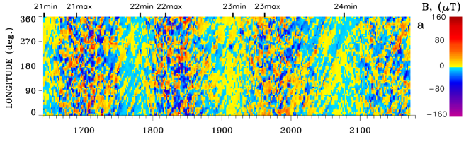
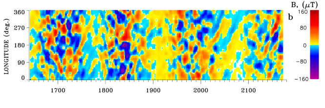
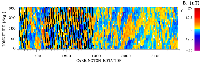
Figure 1.: Longitudinal diagrams. (a) Large-scale photospheric magnetic fields. (b) Large-scale photospheric magnetic fields smoothed by 7x7 CRs. (c) IMF at 1 AU. Red denotes the positive-polarity magnetic fields, blue denotes the negative-polarity magnetic fields. Black denotes the missing data. The maxima and minima of Cycles 21 – 24 are marked at the top.maglon

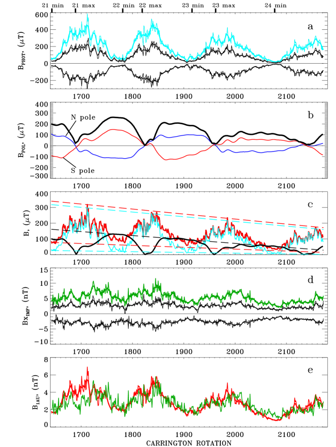
Figure 2.: (a) Photospheric non-polar magnetic fields from the longitudinal diagram Figure maglona. Black denotes the positive- and negative-polarity photospheric magnetic fields, and light blue denotes the sum of their moduli. (b) CR-averaged polar magnetic-field cycle variations at the North (N) and South (S) poles, and the sum of their moduli (black line). (c) Sum of the positive- and negative-polarity photospheric (non-polar) magnetic fields (light blue line) from (a) and the sum of the North and South pole magnetic fields (black line) from (b). Red line denotes the sum of polar and non-polar magnetic fields. (d) IMF measured at 1 AU. Black denotes the CR-averaged positive- and negative-polarity magnetic fields, and green denotes the sum of their moduli. (e) Red line denotes magnetic field at 1 AU calculated from Eq. fmag as the sum the non-polar and polar magnetic fields. Green line denotes the half of the sum of CR-averaged positive- and negative-polarity IMF at 1 AU. In (a), (c), (d), and (e) thin lines correspond to CR-averaged and thick lines to seven CR-averaged data. The maxima and minima of Cycles 21 – 24 are marked at the top.mag

Figure maga shows the cycle changes of the photospheric large-scale magnetic field obtained from the longitudinal distribution of the photospheric magnetic fields by averaging over the latitude from 55 N to 55 S for every CR displayed in Figure maglona. Black denotes the positive- and negative-polarity photospheric magnetic fields, and light blue denotes the sum of their moduli. Thin lines show changes in the CR-averaged magnetic fields and thick lines correspond to the seven CR-averaged data. The maxima and minima of Cycles 21 – 24 are marked at the top of Figure mag. Examination of Figures maglon and mag shows that the magnetic field does not change smoothly from the minimum of solar activity to maximum, but in the form of some impulses. These changes reflect cyclical changes in the structure and strength of the solar global magnetic field (Bilenko, 2012; Bilenko, 2014; Bilenko and Tavastsherna, 2016). The maximum of magnetic field magnitudes decreased and it was the highest in Cycle 21 and the lowest in Cycle 24. The magnetic field strength decrease can be given by

$$B_{max}(t)=317.82-0.30\times t_{CR}\ilabel{fphotmax}$$ (1)

It should be noted, that the minimum values of the magnetic field during solar activity minima also decreased from Cycle 21 to Cycle 24, and it was also the highest in Cycle 21 and the lowest in Cycle 24. We find a regression line

$$B_{min}(t)=26.15-0.47\times t_{CR}\ilabel{fphotmin}$$ (2)

Such cyclic changes in magnetic fields (Figure maga), reflect the time evolution of the toroidal component of the solar global magnetic field. It means that the toroidal component decreases from Cycle 21 to Cycle 24.

Magnetic-field cycle variations at the solar poles are the observational manifestation of the poloidal component of the solar global magnetic field. Figure magb shows CR-averaged magnetic-field variations in the North (blue line) and South (red line) poles. Black line denotes the sum of their moduli. Polar magnetic fields at the North and the South poles diminished from Cycle 21 to Cycle 24. The cyclic changes in magnetic field (Figure magb) reflect the time evolution of the poloidal component of the solar global magnetic field from Cycle 21 to Cycle 24. It means that both components have decreased from Cycle 21 to Cycle 24. The decrease of the polar magnetic field can be expressed by

$$B_{pol}(t)=116.04-0.25\times t_{CR}\ilabel{fpolmin}$$ (3)

The magnetic field in the ecliptic plane can be modeled as the superposition of toroidal and poloidal component cycle variations. The toroidal component dominates at solar maxima and the influence of the poloidal component increases during solar minima. The toroidal component increases during solar maxima because of the enhancement of the active-region magnetic fields. At solar minima, about 60% of the solar sphere above 2 Rs is dominated by polar coronal holes. So, the total magnetic-field strength can be determined as the sum of the non-polar photospheric magnetic fields (toroidal component of the solar global magnetic field, Figure maga) and the polar magnetic field (poloidal component) obtained from Figure magb. Both non-polar (light blue line) and polar (black line) magnetic-field components and their sum (red line) are shown in Figure magc. We detect the magnetic-field components that directly influence on the measured IMF at the Earth’s orbit. It is assumed that the corona is in a steady state from 1 Rs to 1 AU. It should be noted, that both non-polar and polar fields are observed in ecliptic plane from the Earth. So, we can derive the radial component ($B_{x}$) of the IMF from the observed non-polar and polar photospheric magnetic-field strength in ecliptic plane using a relation

$$B(t,r)=\left(\frac{B_{phot+}(t)+B_{phot-}(t)}{2}+\frac{B_{pol_{N}}(t)+B_{pol_{S}}(t)}{2}\right)\times\left(\frac{1}{r}\right)^{2}\ilabel{fmag}$$ (4)

where $B_{phot+}$ and $B_{phot-}$ are the absolute values of the positive- and negative-polarity magnetic fields at the photosphere derived from Figure maglona and shown in Figure maga for each CR, and they represent the toroidal component of the solar magnetic field; $B_{pol_{N}}$ is the absolute value of the observed North polar magnetic field and $B_{pol_{S}}$ is the absolute value of the South polar magnetic field (Figure magb). They represent the poloidal component of the solar global magnetic field; $r$ is the distance from the center of the Sun in units of the solar radius. The different behavior of polar and non-polar magnetic fields is also known from active region (Zharkov, Gavryuseva, and Zharkova, 2007) and coronal hole (Lowder, Qiu, and Leamon, 2017; Bilenko and Tavastsherna, 2016) cycle evolution. Polar and non-polar magnetic fields represent the different components of the solar global magnetic field. Their cycle evolution is different. Therefore, they were included in Equation fmag as separate components.

As noted above, the magnitudes of the toroidal and poloidal magnetic-field components of the solar global magnetic field decreased from Cycle 21 to Cycle 24. We find a regression line for our model (Eq. fmag) magnetic-field cycle maxima

$$B_{m_{max}}(t)=339.93-0.32\times t_{CR}\ilabel{fmagmax}$$ (5)

an expression for the minima can be written as

$$B_{m_{min}}(t)=77.67-0.12\times t_{CR}\ilabel{fmagmin}$$ (6)

In Figure magc, the dashed lines are the regression lines derived in Equations fphotmax, fphotmin, fpolmin, fmagmax, fmagmin.

In Figure magd, the variation of the observed $B_{x}$ component of the IMF at the Earth’s orbit is shown. Black denotes the CR-averaged positive- and negative-polarity magnetic fields, and green denotes the sum of their moduli. Thin lines show CR-averaged IMF and thick lines correspond to the seven CR-averaged data.

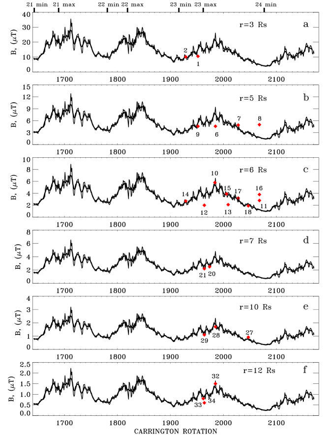
Figure 3.: Model calculated magnetic fields at 3 Rs, 5 Rs, 6 Rs, 7 Rs, 10 Rs, 12 Rs. Red points denote the directly measured IMF (from Table tab1) that are close to these distances. The labels of the points correspond to their number in Table tab1. The maxima and minima of Cycles 21 – 24 are marked at the top.magexmp

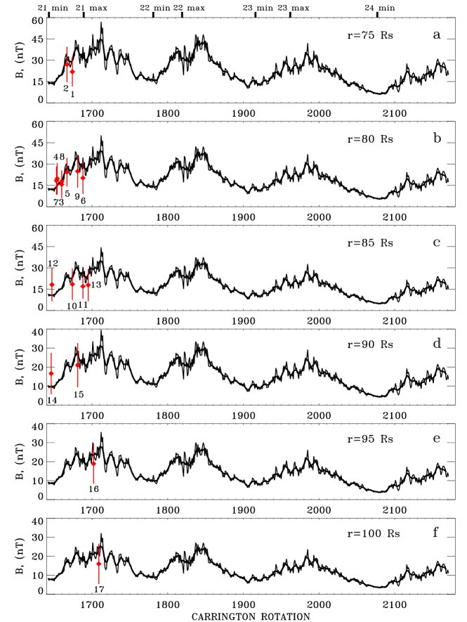
Figure 4.: Model calculated magnetic fields at 75 Rs, 80 Rs, 85 Rs, 90 Rs, 95 Rs, 100 Rs. Red points denote the IMF measured by Helios 1 and Helios 2 spacecraft from Table tab2. The labels of the points correspond to their number in Table tab2. The maxima and minima of Cycles 21 – 24 are marked at the top.maghelios

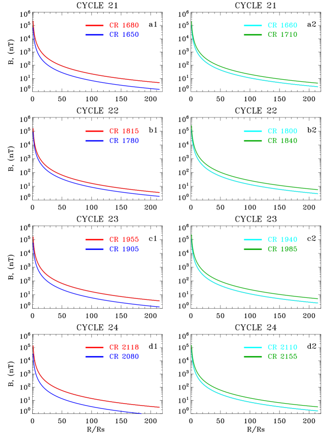
Figure 5.: Magnetic field distributions calculated using our model (Eq. fmag) for different corona activity states. In each panel, the certain CRs are shown for different phases of solar activity. Blue profiles denote solar activity minima corona; red profiles correspond to the solar activity maxima corona; light blue profiles denote solar corona at the rising phases; green profiles denote solar corona at the declining phases.magr

In Figure mage, the magnetic field derived at 1 AU using our model (Eq. fmag) is shown in red color. Green line denotes the half of a sum of CR-averaged positive- and negative-polarity IMF magnetic fields at 1 AU in Cycles 21 – 24. CR-averaged magnetic fields were compared. Both magnetic field retrieved from the photospheric magnetic fields and IMF measured at the Earth’s orbit was calculated the same way. In Eq. fmag, the magnetic fields were used as the half of the sum of the moduli of positive- and negative-polarity non-polar and polar magnetic fields averaged during each CR. Likewise IMF is also the sum of CR-averaged of the moduli of positive- and negative-polarity $B_{x}$ component of the IMF divided by 2. As seen from Figure mage, our model fits $B_{x}$ component of IMF at 1 AU very well particularly during Cycles 23 and 24. From a comparison of the magnetic fields as observed and as calculated from our model, we conclude that our model magnetic-field strength variation adequately explains the major features of the IMF changes during Cycles 21 – 24. However, there are certain differences. The difference is greater during the maximum phase in Cycle 21, but the mismatch is significantly less in the maxima of Cycles 22 and 24 (Figure mage). Some peaks in magnetic fields derived using our model (Equation fmag) coincide with peaks in IMF and some peaks follow the peaks in the IMF. The coincidence between IMF and our model predicted magnetic fields at 1 AU is more pronounced during the declining phases. The reduction of the misalignment between the interplanetary magnetic field and that predicted using our model observed from Cycle 21 to Cycle 24, can be explained by the fact that the quality of observations and measurements of both IMF and solar magnetic fields has significantly improved by now. We have also carried out correlation analysis of our results in order to quantify agreement. The correlation coefficients between the observed IMF and magnetic fields at 1 AU predicted by our model were calculated. The model CR-averaged calculated magnetic fields correlate with IMF at the Earth’s orbit with a coefficient of 0.688. Correlation between seven CR-averaged calculated magnetic fields with seven CR-averaged $B_{x}$ component of the IMF reaches 0.808. For Cycles 21 – 24, the model CR-averaged calculated magnetic fields correlate with CR-averaged $B_{x}$ component of the IMF at the Earth’s orbit with a coefficients of 0.42, 0,69, 0.73, and 0.74 and that for seven CR-averaged values with a coefficients of 0.52, 0,88, 0.85, and 0.88 Again, this implies a very good correlation. So, our model, the Equation fmag, is a good representation of the measured radial ($B_{x}$) component of the IMF in the ecliptic plane.

Figures magexmp, maghelios show some examples of the model magnetic-field evolution during Cycles 21 – 24 calculated at distances of 3 Rs, 5 Rs, 6 Rs, 7 Rs, 10 Rs, and 12 Rs (Figure magexmp) and 75 Rs, 80 Rs, 85 Rs, 90 Rs, 95 Rs, 100 Rs (Figure maghelios). From Figures magexmp, maghelios, it is seen that the magnetic field declines from $\approx 20\mu T$ to $\approx 20nT$ in the distance range from 3 Rs to 100 Rs. The magnetic-field cycle variations derived for different distances and illustrated in Figures magexmp and maghelios should be regarded as a good approximation of the cycle behavior of the radial magnetic-field profiles in the heliosphere. Thus, this method of the magnetic-field calculation is a useful tool for the description of solar corona and interplanetary large-scale magnetic-field cycle evolution at differen distances from the Sun.

Using our model, we can also derive the radial magnetic-field strength profiles for different solar-activity phases and for different distances from the Sun. Figure magr shows magnetic-field radial profiles from 1 Rs to 1 AU. The profiles were derived using Equation fmag as a function of distance for different phases of Cycles 21 – 24. The magnetic-field profiles were calculated for corona activity states: (1) blue lines denote solar-activity minima corona; (2) red lines correspond to the solar activity maxima corona; (3) light blue lines denote the solar corona at the rising phases; (3) green lines denote the solar corona at the declining phases. In each panel, the certain CRs are shown for different phases of solar activity.

4 Coronal Magnetic Field Measurements in Cycles 21 – 24

secmagobs

Table tab1 summarizes the observed magnetic fields (column 6) determined by different authors at different distances (column 4) from the Sun and those calculated using our model, Equation fmag, (column 5) at the same distances and the same time (columns 2, 3). Magnetic-field measured data were taken from the articles cited in column 7.

Table 1.: Magnetic fields observed and that calculated using our model at the same distances from the Sun and the same time.tab1

N	Date	CR	R	B	B	References
			(Rs)	calc.	obs.
				($\mu$T)	($\mu$T)
1	2	3	4	5	6	7
1	25–Jul–1999	1952	3.08	13.99	10.5	Kim et al. (2012)
2	14–Nov–1997	1929	3.33	7.86	10.1	Kim et al. (2012)
3	24–Oct–2003	2009	3.56	11.79	5.6	Kim et al. (2012)
4	1–Apr–2001	1974	4.21	7.70	5.2	Kim et al. (2012)
5	22–Mar–2002	1987	4.3	8.09	1.9	Bemporad et al. (2010)
6	14–Jan–2002	1985	4.82	10.17	4.6	Kim et al. (2012)
7	Mar-Apr–2005	2028	5.0	3.66	4.6-5.2	Ingleby et al. (2007)
8	25–Mar–2008	2068	5.0	1.87	5.0	Gopalswamy et al. (2011)
9	25–Jul–1999	1952	5.55	4.31	4.6	Kim et al. (2012)
10	28–Dec–2001	1984	5.98	5.66	5.8	Kim et al. (2012)
11	5–Apr–2008	2068	6.0	1.3	2.8	Poomvises et al. (2012)
12	15–Jun–2000	1964	6.06	3.42	2.0	Kim et al. (2012)
13	24–Oct–2003	2009	6.10	4.02	2.1	Kim et al. (2012)
14	14–Nov–1997	1929	6.19	2.27	2.7	Kim et al. (2012)
15	16–Aug–2003	2006	6.2	3.75	3.9	Spangler et al. (2005)
16	25–Mar–2008	2068	6.2	1.22	3.8	Gopalswamy et al. (2011)
17	Mar–Apr–2005	2028	6.2	2.38	3.0-3.4	Ingleby et al. (2007)
18	28–Aug–2006	2047	6.2	2.17	1.9	You et al. (2012)
19	5–May–2000	1962	6.35	2.76	3.5	Kim et al. (2012)
20	1–Apr–2001	1974	6.69	3.05	2.5	Kim et al. (2012)
21	15–Jun–2000	1964	7.11	2.49	2.2	Kim et al. (2012)
22	29–Aug–2005	2033	7.5	1.39	2.7	You et al. (2012)
23	14–Jan–2002	1985	7.78	3.90	2.3	Kim et al. (2012)
24	4–May–2000	1962	7.92	1.78	1.8	Kim et al. (2012)
25	25–Jul–1999	1952	8.50	1.84	3.4	Kim et al. (2012)
26	5–May–2000	1962	9.06	1.36	2.1	Kim et al. (2012)
27	30–Aug–2006	2047	9.9	0.85	0.92	You et al. (2012)
28	14–Jan–2002	1985	10.06	2.33	1.7	Kim et al. (2012)
29	15–Jun–2000	1964	10.31	1.18	1.1	Kim et al. (2012)
30	4–Apr–2000	1961	11.46	1.09	2.0	Kim et al. (2012)
31	25–Jul–1999	1952	11.7	0.97	2.1	Kim et al. (2012)
32	14–Jan–2002	1985	12.16	1.59	1.5	Kim et al. (2012)
33	15–Jun–2000	1964	12.27	0.83	0.6	Kim et al. (2012)
34	4–May–2000	1962	12.64	0.7	0.8	Kim et al. (2012)
35	28–Dec–2001	1984	14.89	0.91	1.6	Kim et al. (2012)
36	4–Apr–2000	1961	15.33	0.609	1.0	Kim et al. (2012)
37	5–Apr–2008	2068	120.0	0.003	0.017	Poomvises et al. (2012)

As seen from the Table tab1, the derived magnetic-field values are consistent with other estimates in a similar distance range. In Figure magexmp the model calculated magnetic fields at 3 Rs, 5 Rs, 6 Rs, 7 Rs, 10 Rs, 12 Rs are shown and compared to that measured. Red points denote the directly measured IMF (from Table tab1) that are close to these distances. So, we conclude that our model adequately describes the observed magnetic fields. The comparison of the calculated magnetic field with the observations is complicated by the fact that many of the observations made using different methods and using different solar corona plasma density models. Moreover, large-scale and small-scale irregularities, as well as flows of dense and rarefied plasma move with different speeds in the solar corona and interplanetary space, creating regions of high and sparse density at different distances from the Sun. Even a cursory examination of the measured magnetic fields (Table tab1, column 6) catalogued from the literature (Table tab1, column 7) shows a wide disparity between the determinations of various authors. In spite of the large scatter in the observations, we conclude that they are adequately reproduced by our model. Such a difference can also result from either calibration differences or the influence of different solar activity events. Observed and model magnetic fields differ also because it is hard to distinguish the enhanced magnetic fields, for example in a CME or a streamer region, from the background magnetic field. Our model determines the background magnetic-field strength radial distribution and cycle evolution. The difference in the measured magnetic fields can also result from the dependence of magnetic fields from the selected place of observed event. Hariharan et al. (2014) estimated the magnetic-field strength in the solar corona ahead of and behind the MHD shock front associated with a CME at a distance of $\approx$ 2 Rs. They found magnetic fields of $\approx$ (0.7 – 1.4) $\pm$0.2 G and $\approx$ (1.4 – 2.8) $\pm$0.1 G respectively. Bemporad and Mancuso (2010) determined the plasma parameters of a fast CME-driven shock associated with the solar eruption of 2002 March 22. According to their study, the magnetic field undergoes a compression from a pre-shock value of $\approx$0.02 G up to a post-shock magnetic field of $\approx$0.04 G.

Table 2.: Magnetic fields observed by Helios 1 (H1) and Helios 2 (H2), and that calculated using our model at the same distances from the Sun and the same time.tab2

N	space-	Peri-	CR	R	R	B	B
	craft	helios		RAU	(Rs)	calc.	obs.
						(nT)	(nT)
1	2	3	4	5	6	7	8
1	H2	2–Nov–1978	1674	0.354	76.11	31.17	21.9$\pm$10.3
2	H2	30–Apr–1978	1667	0.356	76.54	28.39	27.0$\pm$12.5
3	H2	26–Oct–1977	1660	0.362	77.83	17.97	17.7$\pm$7.8
4	H2	23–Apr–1977	1654	0.372	79.98	14.86	19.7$\pm$11.1
5	H1	29–Apr–1978	1667	0.373	80.195	25.86	24.3$\pm$10.1
6	H2	9–Nov–1979	1688	0.375	80.625	34.03	20.2$\pm$11.2
7	H1	13–Apr–1977	1653	0.381	81.915	14.5	18.3$\pm$9.9
8	H1	21–Oct–1977	1660	0.387	83.205	15.72	15.7$\pm$9.7
9	H2	7–May–1979	1681	0.389	83.635	30.62	24.9$\pm$11.5
10	H1	5–Nov–1978	1674	0.394	84.71	25.16	18.5$\pm$11.1
11	H1	21–Nov–1979	1688	0.394	84.71	30.83	17.0$\pm$8.7
12	H2	19–Oct–1976	1647	0.396	85.14	11.31	18.2$\pm$11,7
13	H1	29–May–1980	1695	0.398	85.57	25.45	17.9$\pm$11.3
14	H1	5–Oct–1976	1646	0.406	87.29	10.10	16.6$\pm$10.9
15	H1	14–May–1979	1681	0.418	89.87	26.52	21.0$\pm$11.6
16	H1	5–Jan–1980	1702	0.438	94.17	25.54	18.9$\pm$10.6
17	H1	13–Jun–1981	1709	0.469	100.835	19.35	16.0$\pm$10.6

The Helios mission provides one of the best magnetic-field observations. The observations performed by Helios 1 and Helios 2 spacecraft allow one to monitor the IMF conditions in the inner heliosphere from 0.3 to 0.6 AU. We also compare the calculated magnetic-field strength (Equation fmag) with in-situ measurements made by the Helios 1 and Helios 2 spacecraft (Villante, Mariani, and Cirone, 1982).

In Table tab2, the hourly averages of the observed unsigned IMF radial component measured on Helios 1 (H1) and Helios 2 (H2) (column 2) spacecraft are presented (column 8, from Villante, Mariani, and Cirone (1982)). Magnetic fields in column 7 were calculated using the model (Equation fmag) at the same distances (columns 5, 6) and time (columns 3, 4) as it was made in Villante, Mariani, and Cirone (1982). Model calculated magnetic fields at 75 Rs, 80 Rs, 85 Rs, 90 Rs, 95 Rs, and 100 Rs are shown in Figure maghelios. Red points denote the IMF measured by Helios 1 and Helios 2 spacecraft from Table tab2. The agreement between our model predictions and that derived from direct, in-situ measurements is quite satisfactory. From a comparison of Figures mag, magexmp, maghelios, magr and Tables tab1, tab2 of different magnetic-field data as observed and as calculated from our model (Equation fmag), we conclude that our model adequately explains the major features of the magnetic fields at different distances from the Sun during different cycle phases. Therefore, the comparison of the observed magnetic fields with those predicted by our model shows that the magnetic field in the heliosphere is determined by the cycle variations of the sum of poloidal and toroidal components of the solar global magnetic field.

5 Coronal Magnetic Field Models

secmagmod

Magnetic field measurements are important for testing coronal magnetic-field models. Magnetic-field models have played a very important role in the interpretation of different solar activity phenomena and in the study of outward flowing coronal material into the interplanetary space. In this Section, first we summarize various models of deriving the magnetic-field radial distribution. Models discussed below are presented in the form of functions in Figure models. Assuming the conservation of the magnetic flux in the interplanetary space the magnetic field can be continued to arbitrary radial distances $r$ from the Sun (Parker, 1958) by

$$B(r)=B_{s}\times\left(\frac{R_{s}}{r}\right)^{2}\ilabel{fb}$$ (7)

where $B_{s}$ is the magnetic field at the photosphere, obtained using some measurements and assumptions (e.g. Mann et al., 1999) or the magnetic field $B_{s}$ can be composed of the field of an active region and that of the quiet Sun (Warmuth and Mann, 2005). $Rs$ is the radius of the Sun; $r$ is the distance from the center of the Sun in units of the solar radius.

Magnetic-field radial profile can also be represented by an empirical formula of the form

$$B(r)=K\times r^{-\alpha}\ilabel{fk}$$ (8)

where $K$ is a coefficient derived from some approximation of different measurements or models. $r$ is the distance from the center of the Sun in units of the solar radius. A significant number of models were created based on the relation fk. (e.g. Dulk and McLean, 1978; Pätzold et al., 1987; Mancuso et al., 2003; Gopalswamy and Yashiro, 2011). But a large number of models have used the Equation fk formally. The magnetic field values are not included in such formulas.

Traditionally, the problem of a radial magnetic-field distribution has been solved by combining the data obtained using different observations of magnetic fields measured at different times by different methods at different distances from the Sun and on different spacecraft. Then the data are summarized on one curve and fitted by a function like the Equations fb, fk. Such models depend on $r$ only. They do not reflect the actual distribution and cycle evolution of magnetic fields.

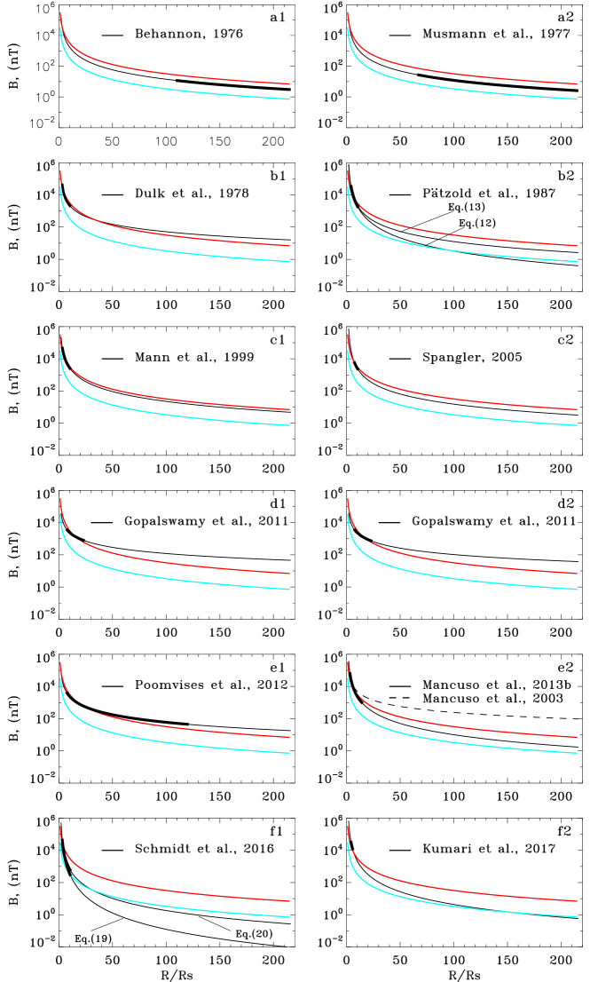
Figure 6.: Magnetic field distributions from 1 Rs to 1 AU calculated for different models (thin black profiles). Thick black lines denote the part of the profiles marking the distances for which the models were created by their authors. Red profiles denote the distribution of magnetic fields using our model for the maximum of Cycle 21 (CR 1712). Blue profiles denote the distribution of magnetic fields using our model for the minimum of Cycle 24 (CR 2079).models

Figure models summarizes radial magnetic-field distributions calculated using different models. The profiles were calculated for radial distances from 1 Rs to 1 AU (thin black profiles). Thick black lines denote the part of the profiles marking the distances for which the models were created by their authors. For comparison, the radial magnetic-field profiles calculated using our model are also shown in Figure models. The magnetic-field radial profiles corresponding to the maximum and minimum solar cycle phases are selected. Red lines denote the radial distribution of magnetic fields calculated using our model for the maximum of Cycle 21 (CR 1712). Blue lines denote the radial distribution of magnetic fields calculated using our model for the minimum of Cycle 24 (CR 2079). Such model calculated magnetic-field profiles can be used as a real magnetic field limitations for different models.

Using measurements of the IMF from several different spacecraft, Behannon (1976) showed that the radial component of magnetic field between 0.5 AU and 5 AU can be fitted by a function

$$B(r)=3.0\times 10^{-5}\left(\frac{r}{216}\right)^{-2}\ilabel{fbehannon1976}$$ (9)

where $B(r)$ is in G, $r$ is the distance from the center of the Sun in units of the solar radius (Figure modelsa1).

Musmann, Neubauer, and Lammers (1977) derived the similar expression for radial variation of the IMF between 0.3 AU and 1.0 AU from Helios 1 data during solar minimum

$$B(r)=1.18\times 10^{-4}r^{-2}\ilabel{fmusmann1977}$$ (10)

where $B(r)$ is in T, $r$ is in units of the solar radius (Figure modelsa2).

One of the most often used model is the empirical formula proposed by Dulk and McLean (1978). Dulk and McLean (1978) concentrated their attention on the magnetic fields above active regions. Using different techniques, and different observational data, they proposed an empirical single parameter formula for magnetic-field radial profile calculation from 1.02 to 10 r/Rs

$$B(r)=0.5\times\left(\frac{r}{Rs}-1\right)^{-1.5}\ilabel{fdulk1978}$$ (11)

where $B(r)$ is in G, $R_{s}$ is the solar radius, $r$ is in units of the solar radius (Figure modelsb1). They pointed out that the magnetic field in the corona can vary from one active region to another by an order of magnitude and that the Equation fdulk1978 is consistent with the different data used to within a factor of about 3.

Pätzold et al. (1987) derived the mean coronal magnetic field from Faraday rotation measurements for $3\leq r\leq 10$ Rs during solar minimum in 1975 – 1976 (Figure modelsb2, Eq.(12)).

$$B(r)=7.9\times 10^{-4}r^{-2.7}\ilabel{fpatzold1987}$$ (12)

The magnetic-field profile derived using a fit to the Faraday rotation data with a dipole term and an interplanetary term is given by an expression (Figure modelsb2, Eq.(13))

$$B(r)=(6r^{-3}+1.18r^{-2})\times 10^{-4}\ilabel{fpatzold1987}$$ (13)

where $B(r)$ is in T, $r$ is in units of the solar radius. Clearly our model profile is closer to the Pätzold et al. (1987) Eq. 13 profile than to the Pätzold et al. (1987) Eq. 12 profile. Pätzold et al. (1987) Eq. 12 profile agrees well with our model profile for solar maximum at shorter distances, but it is lower than our model profile for solar minima.

Mancuso and Spangler (2000) and Spangler (2005) proposed a method for deriving the strength and spatial structure of the solar coronal magnetic field using the observations of the Faraday rotation of radio sources (radio galaxy) occulted by the solar corona at heliocentric distances of 6 – 10 Rs (Figure modelsc2)

$$B(r)=0.06\left(\frac{r}{R_{1}}\right)^{-3}+3.1\left(\frac{r}{R_{1}}\right)^{-2}\ilabel{fspangler2005}$$ (14)

where $B(r)$ is in nanoTesla, $R_{1}$ is one astronomical unit, $r$ is the distance from the Sun in units of the solar radius. In this model, the field changes polarity at the coronal neutral line Spangler (2005).

Several models of the magnetic-field radial distribution were based on CME observations. Gopalswamy and Yashiro (2011) determined the coronal magnetic field strength using white-light coronagraph measures of the shock standoff distance and the radius of curvature of the flux rope during the 2008 March 25 CME. They showed that the radial profile of the magnetic field can be represented by a power law of the form

$$B(r)=p\times r^{-q}\ilabel{fgopals2011}$$ (15)

where $B(r)$ is in G, with $r$ in units of Rs. $p$ and $q$ are the coefficients that depend on the plasma density model. Using Saito (1977) density model with $\gamma=4/3$ and for distances $>9$ Rs they got $p=0.377$ and $q=1.25$ (Figure modelsd1). Using Leblanc, Dulk, and Bougeret (1998) density radial-distribution model they got $p=0.409$ and $q=1.3$ (Figure modelsd2). Gopalswamy and Yashiro (2011) model extrapolation results in a slightly flatter magnetic-field profiles compared to that from our model. Gopalswamy and Yashiro (2011) model magnetic-field profiles agree with our model profiles at shorter distances, but the difference increases with the distance. They determined the coronal magnetic field strength in the heliocentric distance range 6 – 23 solar radii.

Following the standoff-distance method, Poomvises et al. (2012) derived radial magnetic-field strength in the heliocentric distance range from 6 to 120 Rs using data from Coronagraph 2 and Heliospheric Imager I instruments on board the Solar Terrestrial Relations Observatory spacecraft. They found that the radial magnetic-field strength decreases from 28 mG at 6 Rs to 0.17 mG at 120 Rs. They derived magnetic-field profiles in the form of Equation fgopals2011. Using Saito (1977) density mode and $\gamma=4/3$ they got $p=845.870$ and $q=1.59$. Using Leblanc, Dulk, and Bougeret (1998) density radial distribution model they got $p=706.383$ and $q=1.54$. The coefficients are close in value, so the resulting profiles coincide (Figure modelse1).

Several models of the magnetic field radial distribution are based on solar radio emission analysis. Mann et al. (1999) have shown that coronal EIT waves and coronal shock waves associated with type II radio bursts can be used to determine magnetic field in the solar corona. They proposed a model of radial magnetic-field distribution for quiet regions at solar minimum

$$B(r)=2.2\times\left(\frac{Rs}{r}\right)^{2}\ilabel{fman1999}$$ (16)

where $B(r)$ is in G, $r$ is in units of Rs (Figure modelsc1). They determined magnetic field strength between 1.1 – 2.1 solar radii. The model profile matches well our estimates for coronal magnetic field at solar maxima.

Mancuso et al. (2003) studied coronal plasma analyzing type II radio bursts and SOHO Ultra Violet Coronagraph Spectrometer (UVCS) observations. The data sample comprises 37 metric type II radio bursts observed by ground based radio spectrographs in 1999, during the rising phase of Cycle 23. The shock speeds were used to set upper limits to the magnetic field above active regions. An average functional form of the magnetic-field estimates can be represented by the following radial profile, valid between about 1.5 and 2.3 Rs

$$B(r)=(0.6\pm 0.3)\times(r-1)^{-1.2}\ilabel{fmancuso2003}$$ (17)

where $B(r)$ is in G, $r$ is in units of Rs (Figure modelse2).

Coronal magnetic field can be inferred from band-splitting of type II radio bursts (Vrs̆nak et al., 2002). Mancuso and Garzelli (2013a) have also analyzed the band-splitting of type II radio burst to determine the coronal magnetic-field strength in the heliocentric distance range $\approx$1.8 – 2.9 Rs. The same radial profile was obtained higher up in the corona by Mancuso and Garzelli (2013b) based on Faraday rotation measurements of extragalactic radio sources occulted by the solar corona.

$$B(r)=3.76\times r^{-2.29}\ilabel{fvrsnak2002}$$ (18)

where B(r) is in G, $r$ is in units of Rs (Figure modelse2). The profiles derived describe the magnetic field in a range of heliocentric distances from 1.8 Rs to 14 Rs. Clearly our model profile is more in line with the Mancuso and Garzelli (2013a) profile than with the Mancuso et al. (2003) profile.

Comparison of models developed by Behannon (1976), Musmann, Neubauer, and Lammers (1977), Pätzold et al. (1987) (Ed.(13)), Spangler (2005), Mancuso and Garzelli (2013a) (Figure modelsa1, a2, b2 (Eq.13), c2, e2) shows that these model radial profiles and those predicted by our model for the maxima and minima corona states agrees very well. The profiles lie between that calculated for the maxima and minima corona states using our model. The agreement is quite satisfactory, although it is impossible from the profiles to prefer one model above the other.

Schmidt et al. (2016) derived the profile of the strength of the magnetic field in front of a CME-driving shock based on white-light images and the standoff-distance method. They also simulate the CME and its driven shock with a 3-D MHD code. They found good agreement between the two profiles (within $\pm$30%) between 1.8 and 10 Rs. The authors noticed that in their model a magnetic-field profile is decreasing stronger than a monopolar (wind-like) magnetic-field profile $\approx r^{-2}$ and a dipolar profile $\approx r^{-3}$ for an ideal spherically symmetric system. Magnetic-field strength profile derived can be represented as

$$log_{10}B_{calc}(r)=(-3.32\pm 0.5)\times log_{10}(r)+(3.72\pm 0.5)\ilabel{fschmidt2016}$$ (19)

and that simulated with the 3-D MHD code

$$log_{10}B_{sim}(r)=(-2.47\pm 0.5)\times log_{10}(r)+(3.19\pm 0.5)\ilabel{fschmidt2016c}$$ (20)

where $B(r)$ is in mG, $r$ is in units of Rs (Figure modelsf1) The profiles are similar to our model minima profile at shorter distances, but the difference is growing rapidly with increasing distance.

Using radio and white-light observations, Kumari, Ramesh, and Wang (2017) have shown that a single power-law fit is sufficient to describe magnetic fields in the heliocentric distance range $\approx$2.5 – 4.5 Rs

$$B(r)=6.7\times r^{-2.6}\ilabel{fkumari2017}$$ (21)

where B(r) is in G, $r$ is in units of Rs (Figure modelsf2). Resulting profile matches our model profile for magnetic-field maximum at shorter distances and it close to our model profile for magnetic-field minimum at large distances.

From Figure models it is seen, that magnetic-field profiles derived using different models are different. The difference for different models in the variation in magnetic field at 1 AU is an order of magnitude. The main difference between our model and the models described above is that they give only one value for one point at a certain distance from the Sun. They don’t take into consideration the solar cycle magnetic-field evolution. Our model gives more realistic magnetic-field radial distributions taking into account the cycle variations of the solar toroidal and poloidal magnetic fields.

6 Discussion

secdiscussion

In this study a new model has been presented for the radial $B_{x}$ component of the IMF calculation at various distances from the Sun during different solar cycle phases. Results show a rather good match between the measured $B_{x}$ component of the IMF and the model predictions. The magnetic fields from WSO were used in the study. But it is known that the magnetic-field measurements at different observatories are different. To compare data from different observatories, synoptic maps from Wilcox Solar Observatory (WSO), Mount Wilson Observatory (MWO), Kitt Peak (KP), SOLIS, SOHO/MDI, and SDO/HMI measurements of the photospheric field were analyzed by Riley et al. (2014), Virtanen and Mursula (2016), Virtanen and Mursula (2017). The comparison has shown that while there is a general qualitative agreement in the measured data, there are also some significant differences (Riley et al., 2014). The observatories give a similar overall view of the solar magnetic-field and the heliospheric current sheet evolution over four last cycles. However, there are some periods when the data disagree with each other (Virtanen and Mursula, 2016). The differences between the data sets can be due to instrument problems, the choice of the spectral lines that may be formed at different heights and may not measure the same magnetic field, the measurement and treatment of polar fields, for ground-based instruments, atmospheric turbulence can significantly degrade the image quality, the algorithms used to create synoptic maps (Riley et al., 2014). So, the assumption that high-resolution maps from one observatory can be transformed to a lower-resolution map of another by simple averaging is strictly not true. Scaling factors are needed when comparing synoptic maps from different observatories. Therefore, the conversion factors were computed by Riley et al., 2014 that relate measurements of different observatories using both synoptic map pixel-by-pixel and histogram-equating techniques. Virtanen and Mursula (2017) also proposed a method for scaling the photospheric magnetic fields based on the harmonic expansion. The benefit of the harmonic scaling method is that it can be used for data sets of different resolutions.

WSO provides the longest and most homogenous magnetic-field observations, a lot of investigations based on WSO data. But WSO provides the lowest values for photospheric magnetic field data, and thus a weaker coronal magnetic-field strength, than the Mount Wilson Observatory, Kitt Peak, SOLIS, SOHO/MDI, and SDO/HMI (Riley et al., 2014). The size of a WSO pixel is 3 minutes of arc in sky coordinates, or 180 arc sec, which at disk-center represents about 126 Mm, or about 10 degrees of heliographic longitude. Such large pixels cannot resolve active regions so most active region flux is not detected by WSO. So, the WSO’s very low spatial resolution can be a part of the explanation of the good match, because it was found that the origin of IMF is the large-scale photospheric magnetic fields (Ness and Wilcox, 1964; Ness and Wilcox, 1965; Ness and Wilcox, 1966; Severny et al., 1970). IMF evolves in response to the solar coronal and photospheric magnetic fields at its base. The source of the interplanetary-sector structure is associated with large-scale photospheric magnetic-field patterns, the patterns of weak photospheric background fields (Wilcox, 1968, Wilcox and Ness, 1967) with the area equal to about one-fourth the area of the solar disk (Scherrer and Wilcox, 1972), or according to Plyusnina 1985 the size of unipolar photospheric magnetic-field pattern is on the average larger than $40^{\circ}$. Therefore, such a good coincidence between the measured magnetic field and that predicted by the model is largely because of WSO’s low-resolution measurements. The active region total flux is unresolved. The WSO measured magnetic field is the large-scale field that form and govern IMF.

It should be noted, that the photospheric magnetic fields and IMF are measured from the Earth and Earth’s orbit. Only flux from different latitudes that is detected at the Earth is considered. This does not imply that approximately the same proportion of low- and high-latitude fields contribute to the IMF $B_{x}$ component. We don’t see the real radial polar magnetic field from the Earth. Since the value of the polar magnetic field observed from the Earth is used, not the full magnetic flux of the polar regions is really measured, but only the tangential component of the polar magnetic field of the visible polar area. The contribution of polar regions is far less than that of low-latitude fields especially during maxima phases, when the polar region influence is negligible despite the fact that the polar flux is much more unipolar than the low-latitude flux over most of the cycle. The role of polar fields increases during minima phases. The central part of the visible solar disc contributes the major amount of magnetic flux to the magnetic field measured at the Earth. Scherrer et al. (1977) have shown that about half the contribution to the mean (sun-as-a-star) field comes from the center 35% of the disc area.

The active region magnetic-field influence on the IMF is insignificant beyond source surface. It was found that the origin of IMF is the large-scale photospheric magnetic fields. The source of the interplanetary-sector structure is associated with the pattern of weak photospheric background fields (Wilcox, 1968). The background solar magnetic field is represented predominantly by a radial field (as seen from vectormagnetograms and EUV images). It should be stressed, that it does not show significant variations with latitude. The independence of latitude was also observed by Ulysses in the radial component of IMF (Forsyth et al., 1996; Smith and Balogh, 1995; Balogh et al., 1995). But, as already mentioned earlier, both the photospheric magnetic field and IMF are measured from the Earth and the Earth’s orbit. Hence, the contribution of the unipolar regions to the total magnetic flux that reaches the Earth is also mainly from the central solar region.

Finally, it should be noted that the photospheric magnetic fields must be accurate determined as they are used to calculate coronal magnetic fields and IMF. So, the magnetic-field measurements from other observatories can be used with appropriate scaling factor to calculate the IMF at various distances from the Sun during different cycle phases.

7 Conclusion

secconclusion

A new model has been proposed for magnetic field determination at different distances from the Sun throughout solar cycles. The model depend on the observed large-scale photospheric magnetic fields. The direct observations of the large-scale non-polar photospheric ($\pm 55^{\circ}$) and polar (from $55^{\circ}$ N to $90^{\circ}$ N and from $55^{\circ}$ S to $90^{\circ}$ S) magnetic fields were used, which are the visible manifestations of cyclic changes in the toroidal and poloidal components of the solar global magnetic field. The model magnetic field is determined as the sum of the non-polar photospheric magnetic field (toroidal component of the solar global magnetic field) and the polar magnetic field (poloidal component) cycle variations.

The agreement between our model predictions and magnetic fields derived from direct, in-situ, measurements at different distances from the Sun and at different time is quite satisfactory. From a comparison of the magnetic fields as observed and as calculated from our model at 1 AU, we also conclude that the model magnetic-field strength variation adequately explains the major features of the IMF $B_{x}$ component cycle evolution at the Earth’s orbit. The model CR-averaged calculated magnetic fields correlate with CR-averaged IMF $B_{x}$ component at the Earth’s orbit with a coefficient of 0.688. Correlation between seven CR-averaged calculated magnetic fields with IMF $B_{x}$ component reaches 0.808. For Cycles 21 – 24, the model CR-averaged calculated magnetic fields correlate with CR-averaged IMF $B_{x}$ component at the Earth’s orbit with a coefficients of 0.42, 0,69, 0.73, and 0.74 and that for seven CR-averaged values with a coefficients of 0.52, 0,88, 0.85, and 0.88

The magnetic-field cycle variations derived for different distances should be regarded as a good approximation of the radial cycle behavior of the magnetic fields in the heliosphere. Thus, this method of the magnetic-field calculation is a useful tool for the description of solar corona and interplanetary large-scale magnetic-field cycle evolution at differen distances from the Sun. So, the model should be regarded as a good approximation of the cycle behavior of the magnetic field in the heliosphere.

Magnetic-field profiles derived from our model are similar to those of empirical models and previous estimates. The major difference between our model and the models described above is that they give only one value for one point at a certain distance from the Sun. They don’t take into consideration the solar cycle magnetic-field evolution. Our model gives more realistic magnetic-field radial distributions taking into account the cycle variations of the solar toroidal and poloidal magnetic fields.

A particularly interesting finding has been the decrease in maximum of the photospheric magnetic-field magnitudes from Cycle 21 to Cycle 24. It should be noted that the minimum values of the magnetic field in the solar activity minima are also decreased from Cycle 21 to Cycle 24. The polar magnetic field also decreased. Such changes in magnetic fields reflect the time evolution of the toroidal and poloidal components of the solar global magnetic field. It means that both components and therefore, the solar global magnetic field decreased from Cycle 21 to Cycle 24.

Acknowledgments

The author express the appreciation to the anonymous referee for a very thorough and helpful review of the paper.

Wilcox Solar Observatory data used in this study was obtained via the web site $http://wso.stanford.edu\,at\,2018:03:11\,01:13:34$ PST courtesy of J.T. Hoeksema. The Wilcox Solar Observatory is currently supported by NASA.

Data on IMF were obtained from multi-source OMNI 2 data base via the web site $https://omniweb.gsfc.nasa.gov/ow.html$. The author thanks the GSFC/SPDF and OMNIWeb for the opportunity to use this data.

References

- Akhmedov et al. (1982) Akhmedov, S.B., Gelfreikh, G.B., Bogod, V.M., Korzhavin, A.N.: 1982, The measurement of magnetic fields in the solar atmosphere above sunspots using gyroresonance emission. Sol. Phys. 79, 41. DOI.
- Balogh et al. (1995) Balogh, A., Smith, E.J., Tsurutani, B.T., Southwood, D.J., Forsyth, R.J., Horbury, T.S.: 1995, The heliospheric magnetic field over the south polar region of the Sun. Science 268, 1007. DOI.
- Banaszkiewicz, Axford, and McKenzie (1998) Banaszkiewicz, M., Axford, W.I., McKenzie, J.F.: 1998, An analitycal solar magnetic field model. A&A 337, 940.
- Behannon (1976) Behannon, K.W.: 1976, Mariner 10 interplanetary magnetic field results. In: in D.J. Williams (ed), Physics of Solar Planetary Environments; Proceedings of the International Symposium on Solar-Terrestrial Physics, Am. Geophys. Union. A77-44201 20-88 1, 332.
- Bemporad and Mancuso (2010) Bemporad, A., Mancuso, S.: 2010, First complete determination of plasma physical parameters across a coronal mass ejection-driven shock. ApJ 720, 130. DOI.
- Bemporad et al. (2016) Bemporad, A., Susino, R., Frassati, F., Fineschi, S.: 2016, Measuring coronal magnetic field with remote sensing observations of shock waves. Fronties in Astronomy and Space Science 3, id.17. DOI.
- Bilenko (2012) Bilenko, I.A.: 2012, Formation of coronal mass ejections at different phases of solar activity. Geomagnetism and Aeronomy 52, 1005. DOI.
- Bilenko (2014) Bilenko, I.A.: 2014, Influence of the solar global magnetic-field structure evolution on CMEs. Sol. Phys. 289, 4209. DOI.
- Bilenko and Tavastsherna (2016) Bilenko, I.A., Tavastsherna, K.S.: 2016, Coronal hole and solar global magnetic field evolution in 1976 - 2012 . Sol. Phys. 291, 2329. DOI.
- Bogod and Yasnov (2008) Bogod, V.M., Yasnov, L.V.: 2008, Vertical structure of the magnetic field in active regions of the Sun at coronal heights. Cosmic Res. 46, 309. DOI.
- Bogod and Yasnov (2016) Bogod, V.M., Yasnov, L.V.: 2016, Determination of the structure of the coronal magnetic field using microwave polarization measurements. Sol. Phys. 291, 3317. DOI.
- Bogod, Stupishin, and Yasnov (2012) Bogod, V.M., Stupishin, A.G., Yasnov, L.V.: 2012, On magnetic fields of active regions at coronal heights. Sol. Phys. 276, 61. DOI.
- Brosius and White (2006) Brosius, J.W., White, S.M.: 2006, Radio measurements of the height of strong coronal magnetic fields above sunspots at the solar limb. ApJ 641, L69. DOI.
- Cho et al. (2007) Cho, K.-S., Lee, J., Gary, D.E., Moon, Y.-J., Park, Y.D.: 2007, Magnetic field strength in the solar corona from type II band splitting. ApJ 665, 799. DOI.
- Dulk and McLean (1978) Dulk, G.A., McLean, D.J.: 1978, Coronal magnetic fields. Sol. Phys. 57, 279. DOI.
- Duvall et al. (1977) Duvall, T.L.J., Wilcox, J.M., Svalgaard, L., Scherrer, P.H., McIntosh, P.S.: 1977, Comparison of Ha synoptic charts with the large-scale solar magnetic field as observed at Stanford. Sol. Phys. 55, 63. DOI.
- Forsyth et al. (1996) Forsyth, R.J., Balogh, A., Horbury, T.S., Erdoes, G., Smith, E.J., Burton, M.E.: 1996, The heliospheric magnetic field at solar minimum: ULYSSES observations from pole to pole. A&A 316, 287.
- Gelfreikh, Peterova, and Riabov (1987) Gelfreikh, G.B., Peterova, N.G., Riabov, B.I.: 1987, Measurements of magnetic fields in solar corona as based on the radio observations of the inversion of polarization of local sources at microwaves. Sol. Phys. 108, 89. DOI.
- Gibson and Bagenal (1995) Gibson, S.E., Bagenal, F.: 1995, Large-scale magnetic field and density distribution in the solar minimum corona. J. Geophys. Res. 100, 19865. DOI.
- Gopalswamy and Yashiro (2011) Gopalswamy, N., Yashiro, S.: 2011, The strength and radial profile of the coronal magnetic field from the standoff distance of a coronal mass ejection-driven shock. ApJ 736, L17(5pp). DOI.
- Gopalswamy et al. (2012) Gopalswamy, N., Nitta, N., Akiyama, S., Mäkelä, P., Yashiro, S.: 2012, Coronal magnetic field measurement from EUV images made by the Solar Dynamics Observatory. ApJ 744, 72(7pp). DOI.
- Hariharan et al. (2014) Hariharan, K., Ramesh, R., Kishore, P., Kathiravan, C., Gopalswamy, N.: 2014, An estimate of the coronal magnetic field near a solar coronal mass ejection from low-frequency radio observations. ApJ 795, 9pp. DOI.
- Hoeksema and Scherrer (1986) Hoeksema, J.T., Scherrer, P.H.: 1986, An atlas of photospheric magnetic field observations and computed coronal magnetic fields: 1976-1985. Sol. Phys. 105, 205. DOI.
- Ingleby, Spangler, and Whiting (2007) Ingleby, L.D., Spangler, S.R., Whiting, C.A.: 2007, Probing the large-scale plasma structure of the solar corona with Faraday rotation measurements. ApJ 668, 520. DOI.
- Kaltman et al. (2012) Kaltman, T.I., Bogod, V.M., Stupishin, A.G., Yasnov, L.V.: 2012, The altitude structure of the coronal magnetic field of AR 10933. Astron. Rep. 56, 790. DOI.
- Kim et al. (2012) Kim, R.-S., Gopalswamy, N., Moon, Y.-J., Cho, K.S., S. Yashiro, S.: 2012, Magnetic field strength in the upper solar corona using white-light shock structures surrounding coronal mass ejections. ApJ 746, 118(8pp). DOI.
- King and Papitashvili (2005) King, J.H., Papitashvili, N.E.: 2005, Solar Wind Spatial Scales in and Comparisons of Hourly Wind and ACE Plasma and Magnetic Field Data. J. Geophys. Res. 110, A02104. DOI.
- Kumari, Ramesh, and Wang (2017) Kumari, A., Ramesh, C. R. Kathiravan, Wang, T.J.: 2017, Addendum to: strength of the solar coronal magnetic field - a comparison of independent estimates using contemporaneous radio and white-light observations. Sol. Phys. 292, article id.177. DOI.
- Leblanc, Dulk, and Bougeret (1998) Leblanc, Y., Dulk, G.A., Bougeret, J.-L.: 1998, Tracing the electron density from the corona to 1 AU. Sol. Phys. 183, 165. DOI.
- Lin, Kuhn, and Coulter (2004) Lin, H., Kuhn, J.R., Coulter, R.: 2004, Coronal magnetic field measurements. ApJ 613, L177. DOI.
- Lin, Penn, and Tomczyk (2000) Lin, H., Penn, M.J., Tomczyk, S.: 2000, A new precise measurement of the coronal magnetic field strength. ApJ 541, L83. DOI.
- Lowder, Qiu, and Leamon (2017) Lowder, C., Qiu, J., Leamon, R.: 2017, Coronal holes and open magnetic flux over cycles 23 and 24. Sol. Phys. 292, article id. 18, 23. DOI.
- Mancuso and Garzelli (2013a) Mancuso, S., Garzelli, M.V.: 2013a, Coronal magnetic field strength from type II radio emission: complementarity with Faraday rotation measurements. A&A 560, L1. DOI.
- Mancuso and Garzelli (2013b) Mancuso, S., Garzelli, M.V.: 2013b, Radial profile of the inner heliospheric magnetic field as deduced from Faraday rotation observations. A&A 553, A100. DOI.