Emergent dimerization and localization in disordered quantum chains

Abstract

We uncover a novel mechanism for inducing a gapful phase in interacting many-body quantum chains. The mechanism is nonperturbative, being triggered only in the presence of both strong interactions and strong aperiodic (disordered) modulation. In the context of the critical antiferromagnetic spin-1/2 XXZ chain, we identify an emerging dimerization which removes the system from criticality and stabilizes the novel phase. This mechanism is shown to be quite general in strongly interacting quantum chains in the presence of strongly modulated quasiperiodic disorder which is, surprisingly, perturbatively irrelevant. Finally, we also characterize the associated quantum phase transition via the corresponding critical exponents and thermodynamic properties.

I Introduction

The presence of quenched disorder in noninteracting quantum systems may lead to localization phenomena both in the case of random elements, as in the Anderson model(Anderson, 1958), and of deterministic quasiperiodic modulation, as in the Aubry–André model(Aubry and André, 1980). Recently, in the context of many-body localization(Basko et al., 2006; Nandkishore and Huse, 2015; Altman and Vosk, 2015), the interplay between interactions and deterministic disorder has gained renewed interest both from the theoretical point of view(Iyer et al., 2013; Nag and Garg, 2017; Khemani et al., 2017; Lee et al., 2017) and from its experimental realization in ultracold atom systems(Roati et al., 2008; Schreiber et al., 2015; Lüschen et al., 2017; Bordia et al., 2017).

These studies usually deal with translational-symmetry breaking introduced by an incommensurate potential. In contrast, here we consider the effects of aperiodic modulation introduced in the exchange couplings. We show that, for a certain class of coupling arrangements, the ground state is delocalized for weak interactions even in the strong-modulation limit, but sufficiently strong interactions induce a novel zero-temperature transition to an emergent aperiodic dimer phase with localized low-energy excitations.

For concreteness, we focus on the spin-$\frac{1}{2}$ XXZ chain defined by the Hamiltonian

$$H=\sum_{i=1}^{L-1}J_{i}\left(S_{i}^{x}S_{i+1}^{x}+S_{i}^{y}S_{i+1}^{y}+\Delta S_{i}^{z}S_{i+1}^{z}\right),$$ (1)

in which $S_{i}^{x,y,z}$ are spin-$\frac{1}{2}$ operators and we assume antiferromagnetic couplings $J_{i}>0$ with an easy-plane anisotropy $-1/\sqrt{2}<\Delta\leq 1$. Via a Jordan-Wigner transformation, it is well-known that (1) also describes one-dimensional spinless fermions with hopping amplitude $\propto J_{i}$ and interaction strength $\propto J_{i}\Delta$. Thus, we will also refer to the anisotropy parameter $\Delta$ as the interaction strength.

In the thermodynamic limit, the ground state of the uniform (clean) system ($J_{i}\equiv J$) is critical and low-energy excitations are described as a spin (Luttinger) liquid with a dynamical critical exponent $z_{{\rm clean}}=1$. It is perturbatively unstable against dimerization (i.e, alternating couplings $J_{i}\equiv\left[1+\frac{1}{2}(-1)^{i}\delta\right]J$, with a dimerization strength $\delta$), which produces an energy gap $\Delta E\sim\left|\delta\right|$ above the ground state and a finite correlation length diverging as $\xi\sim\left|\delta\right|^{-\nu}$ for $\delta\rightarrow 0$ with a critical exponent(Luther and Peschel, 1975; Kossow et al., 2012) $\nu=2\left(\pi-\arccos\Delta\right)/(3\pi-4\arccos\Delta)$.

The clean critical system is also perturbatively unstable against random disorder (i.e, couplings $J_{i}$ independently chosen from a probability distribution with a nonzero width $\delta J$), as dictated by the Harris criterion(Harris, 1974; Doty and Fisher, 1992). However, there is no energy gap and the Luttinger liquid is replaced by a random-singlet spin liquid whose low-energy physics is governed by a critical infinite-randomness fixed point with an infinite dynamical critical exponent(Fisher, 1994; Hoyos et al., 2007). Introducing correlations between the random couplings can either slightly change the critical behavior of the infinite-randomness fixed point(Rieger and Iglói, 1999) or stabilize a line of finite-disorder critical points along which the dynamical exponent remains finite but larger than one(Hoyos et al., 2011; Getelina et al., 2016).

The effects of deterministic disorder are expected to be similar. Indeed, for perturbatively relevant geometric fluctuations, the ground state of the clean system is replaced by a critical self-similar version of a random-singlet state with an infinite dynamical exponent, just as for uncorrelated random disorder(Vieira, 2005a, b). For marginally relevant geometric fluctuations, on the other hand, the dynamical exponent remains finite but larger than one, just as for the line of finite-disorder fixed points appearing in correlated random aperiodicity.

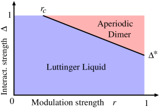
Figure 1: Schematic phase diagram of the XXZ spin-$\frac{1}{2}$ chain Eq. (1) in the presence of perturbatively irrelevant deterministic aperiodicity. The anisotropy parameter $\Delta$ parameterizes the strength of the interactions while the modulation $r$ parameterizes the strength of the aperiodicity. For the aperiodic sequence defined in Eq. (2), $r_{c}\approx 0.13$ and $\Delta^{*}\approx 0.69$.

However, the case of perturbatively irrelevant deterministic disorder has not been previously studied in detail. Evidently, for weak modulation $r$ of the aperiodic couplings the system still corresponds to a critical Luttinger liquid. In this paper we show that, surprisingly, increasing $r$ beyond the perturbative limit ($r>r_{c}$) induces the opening of an energy gap in the spectrum, as depicted in Fig. 1. To the best of our knowledge, this is the first verification that an aperiodic perturbation (random or deterministic) induces such an effect in a critical system. Furthermore, this effect is only possible in the presence of sufficiently strong interactions (anisotropy parameter $\Delta>\Delta^{*}$). Finally, we show that this gap is related to an emergent dimerization of effective couplings in the low-energy limit, characterizing an aperiodic dimer phase, with localized low-energy excitations.

This paper is organized as follows. In Sec. II, we introduce the bond sequence at which we focus, representing the class of aperiodic sequences defined in App. A, and discuss its perturbative effects on the ground state of the quantum XXZ chain. In Sec. III, we investigate the opposite limit of strong modulation. The results of numerical calculations confirming the predictions in both limits are reported in Sec. IV. Finally, Sec. V presents a discussion of our results, while some technical details are relegated to Apps. B and C.

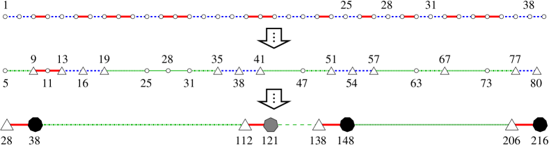
Figure 2: The upper lattice shows the leftmost portion of the aperiodic sequence of bonds in Eq. (2). Dashed blue lines represent weak ($J^{(a)}$) couplings and solid red lines represent strong ($J^{(b)}$) couplings. The middle lattice is obtained after the first two renormalization steps (consisting in decimating the strong bonds $J^{(b)}$ and all remaining weak bonds $J^{\left(a\right)}$). The lower lattice shows the effective chain produced in the latest stages of the SDRG method in the Heisenberg limit $\Delta=1$. Notice the alternating pattern of strong (red/short/thick/solid) and weak (green/long/thin/broken) effective couplings, revealing an emergent dimerization. Circles and polygons represent real spins and low-energy effective spin-1/2 degrees of freedom (effective spins), respectively. In the latter case, the number of sides (3, 7, or 9) is the number of real spins within. The numbers indicate the original position of the central real spin.

II Deterministic aperiodic sequences and their perturbative relevance

Let us start by defining the main bond sequence $\{J_{i}\}$ investigated in this work. Consider the following substitution rule for letter pairs:

$$\left\{\begin{array}[]{ccc}aa&\rightarrow&aa\,ba\,ab\,ab\,ba\\ ab&\rightarrow&aa\,ba\,ab\\ ba&\rightarrow&ab\,ba\,aa\,ab\,ba\end{array}\right..$$ (2)

Iterating this rule, starting from a single pair $aa$, we obtain an aperiodic sequence of letters $a$ and $b$ which we associate, respectively, with different bond values $J^{(a)}$ and $J^{(b)}$ of our aperiodic XXZ chain. The modulation of the aperiodic couplings is quantified by $r\equiv 1-J^{(a)}/J^{(b)}$. As detailed in App. A, the sequence in Eq. (2) represents a large family of sequences exhibiting the same qualitative behavior, and was selected on the basis of convenience for numerical calculations, since it gives rise to a relatively large energy gap to the lowest excited states.

We emphasize the fact that there is no average dimerization induced in the bonds $J_{i}$ by the substitution rule (2), the average couplings being the same at odd and even positions along the chain. Therefore, no gap is expected for weak modulation $r$.

We studied the weak-modulation effects of couplings chosen from the sequence in Eq. (2) by adapting the perturbative renormalization-group (RG) method of Vidal, Mouhanna and Giamarchi(Vidal et al., 1999, 2001) (see also Ref. Hida, 2001) to the XXZ chain (1). In this approach, as described in Appendix B, it is found that the relevant effects of bond disorder on the corresponding low-energy field theory describing the clean system are determined by the behavior of the Fourier transform $\tilde{J}\left(Q\right)$ of the bond sequence in the neighborhood of $Q=2k_{f}=\pi$, where $k_{f}=\pi/2$ gives the location of the corresponding Fermi level. When the integrated Fourier weight around $Q=\pi$ grows sufficiently slowly, the perturbative RG approach predicts that weak modulation is irrelevant. For $0\leq\Delta\leq 1$, this is precisely the case of the whole family of aperiodic sequences represented by the one in Eq. (2). This is consistent with Luck’s generalization(Luck, 1993a) of the Harris criterion(Harris, 1974) for the perturbative relevance of aperiodicity on the critical behavior of physical systems.

III The XXZ chain with an aperiodic bond distribution: strong modulation

Having determined the perturbative irrelevance of our aperiodic system, we now study its low-energy properties in the strong (non-perturbative) modulation regime $r\approx 1$ where an adaptation of the strong-disorder real-space RG (SDRG) method(Ma et al., 1979; Bhatt and Lee, 1982) for aperiodic XXZ spin chains(Vieira, 2005a, b) can be used. In this approach, one identifies clusters of strongly coupled spins (the clusters connected by solid red lines in Fig.2). For $r\approx 1$, it is a good approximation to keep only the low-energy state of these “molecules” which is either a singlet (for $m$ even) or a doublet (for $m$ odd), where $m$ is the number of spins in the molecule. For a singlet, the molecule is simply removed from the effective chain since its excitations are costly. In the case of a doublet, the molecule is then replaced by a new effective spin-$\frac{1}{2}$ degree of freedom (see the transition from the upper to the middle lattice in Fig.2). The new renormalized (and weaker) bonds connecting the remaining spins in the lattice are obtained via perturbation theory. Repeating this process, the energy scale is reduced and the spatial distribution of couplings may reach a self-similar fixed point, making it possible to write recursion relations for the effective couplings and to obtain an approximate low-energy spectrum. (See Appendix A of Ref. Vieira, 2005b for details.) We mention that this method was extended to higher spins(Casa Grande et al., 2014), to the quantum Ising chain(Oliveira Filho et al., 2012), to the contact process (Barghathi et al., 2014), and it can also be used to investigate entanglement properties(Iglói et al., 2007; Juhász and Zimborás, 2007).

Let us now turn our attention back to the perturbatively irrelevant sequence Eq. (2), to which we numerically apply the SDRG method. Here no self-similar fixed-point exists. In the noninteracting XX limit ($\Delta=0$), we find that, for any modulation strength $0<r<1$, the effective couplings approach each other as the RG procedure is iterated. In other words, the SDRG flows towards the clean fixed point $r^{*}=0$. Therefore, we conclude that our aperiodicity is irrelevant in both the weak and the strong modulation regimes, as depicted in Fig. 1.

In contrast, the SDRG flow completely changes its character for $\Delta>\Delta^{*}\approx 0.69$. As illustrated in Fig. 2 for $\Delta=1$, the effective low-energy chain exhibits an emergent dimerization pattern alternating weak and strong effective couplings. Surprisingly, all the strong couplings have the same magnitude, so that an energy gap in the spectrum must exist above the ground state, and we find it to scale as

$$\Delta E/J^{(b)}\sim\left(J^{(a)}/J^{(b)}\right)^{2}=\left(1-r\right)^{2}.$$ (3)

On the other hand, the weak couplings follow a broad distribution of lengths $l$ and strengths $J_{{\rm weak}}$, which are related by

$$J_{{\rm weak}}\sim\exp(-\mu\ln^{2}(l/l_{0})),$$ (4)

the constants $\mu$ and $l_{0}$ depending only on the anisotropy $\Delta$. For more details, see App. C.

In the strong-modulation limit of the Heisenberg chain, the effective Hamiltonian of a system with $\ell$ effective spins ($\ell$ even for convenience) can be written as

$$\tilde{H}=\tilde{J}_{\text{strong}}\sum_{j=1}^{\ell/2}\vec{S}_{2j-1}\cdot\vec{S}_{2j}+\sum_{j=1}^{\ell/2-1}\tilde{J}_{j}\vec{S}_{2j}\cdot\vec{S}_{2j+1},$$ (5)

in which all strong effective couplings $\tilde{J}_{\text{strong}}$ have the same intensity, much larger than the intensities of the weak effective couplings $\tilde{J}_{j}$, all of which can be calculated from a numerical implementation of the SDRG scheme.

If all $\tilde{J}_{j}$ were zero, the ground state could be written as

$$\left|\Psi_{0}\right\rangle=\left|s\right\rangle_{1,2}\otimes\left|s\right\rangle_{3,4}\otimes\left|s\right\rangle_{5,6}\otimes\cdots\otimes\left|s\right\rangle_{\ell-1,\ell},$$ (6)

where $\left|s\right\rangle_{i,j}$ is a spin-$\frac{1}{2}$ singlet between the effective spins $i$ and $j$. The perturbative effect of the weak effective couplings on the ground state is to provide a second-order correction to the ground-state energy.

Again if all $\tilde{J}_{j}$ were zero, the $\frac{3}{2}\ell$ degenerate lowest-energy excitations would correspond to states

$$\left|j_{S^{z}}\right\rangle=\left(\bigotimes_{i\neq j}\left|s\right\rangle_{2i-1,2i}\right)\otimes\left|t_{S^{z}}\right\rangle_{2j-1,2j},$$ (7)

with $\left|t_{S^{z}}\right\rangle_{i,j}$ denoting the triplet state between the effective spins $i$ and $j$, and $S^{z}=-1,\ 0,\ 1$. The degeneracy is then lifted when the weak couplings are turned on. The first-order perturbative effective Hamiltonian for the lowest-energy many-body band is a simple tight-binding chain with zero onsite potential describing the hoppings of the “triplons” over the dimers,

$$\tilde{H}_{\text{low}}=-\frac{1}{2}\sum_{j=1}^{\ell/2-1}\tilde{J_{j}}\left(\left|j_{S^{z}}\right\rangle\left\langle j+1_{S^{z}}\right|+\left|j+1_{S^{z}}\right\rangle\left\langle j_{S^{z}}\right|\right),$$ (8)

where an unimportant constant (the average gap to the ground state) was neglected.

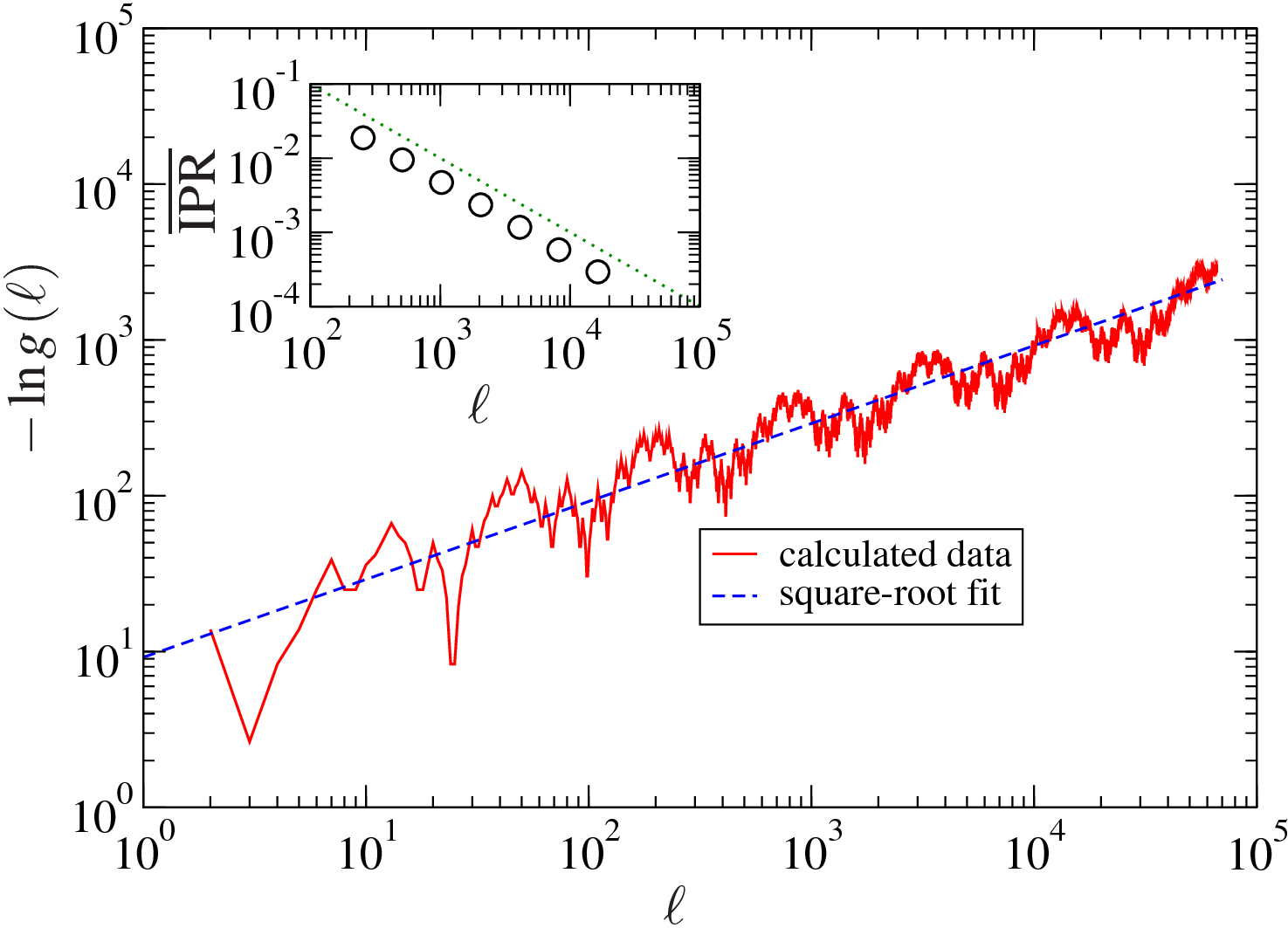
Figure 3: Main plot: Logarithm of the conductance as a function of the number of effective spins $\ell$ of the effective tight-binding Hamiltonian (8) describing the lowest-energy many-body excitation band of the Heisenberg chain with couplings following the sequence in Eq. (2) in the strong-modulation limit. The blue dashed curve is a fit given by $-9.20\ell^{\psi}$, with $\psi=\frac{1}{2}$. The chemical potential corresponds to the band center. Inset: Average inverse participation as a function of the effective system size. The green dotted line is proportional to $1/\ell$.

We now ask whether the triplons are localized or not. From the set $\left\{\tilde{J}_{j}\right\}$ provided by the SDRG approach, and following the analysis in Ref. Javan Mard et al., 2014, we study, as a function of the effective system size $\ell$, the zero-temperature conductance when the chemical potential corresponds to the center of the first excited band,

$$g\left(\ell\right)=\frac{4t_{\ell}^{2}}{\left(1-t_{\ell}^{2}\right)^{2}},$$ (9)

where

$$t_{\ell}=-\frac{1}{2}\frac{\tilde{J}_{1}\tilde{J}_{3}\tilde{J}_{5}\cdots\tilde{J}_{\frac{1}{2}\ell-1}}{\tilde{J}_{2}\tilde{J}_{4}\tilde{J}_{6}\cdots\tilde{J}_{\frac{1}{2}\ell-2}}$$ (10)

is the system transmission coefficient (for convenience, we are assuming that $\frac{1}{2}\ell$ is even). We choose this particular chemical potential because it is expected to probe the least localized state in the band (Eggarter and Riedinger, 1978). As shown in Fig. 3, $g(\ell)$ is compatible with the stretched-exponential scaling form

$$\ln g\left(\ell\right)\sim-\ell^{\psi},$$ (11)

with a tunneling exponent(Javan Mard et al., 2014) $\psi=\frac{1}{2}$. (The superimposed log-periodic oscillations are a common feature of aperiodicity generated by substitution rules.) As shown in Refs. Vieira, 2005a, b, in the present context the tunneling exponent $\psi$ is related to the pair wandering exponent $\omega_{\text{weak}}$ of the effective weak couplings $\{\tilde{J}_{i}\}$ via $\psi=\omega_{\text{weak}}$. We have explicitly verified that $\omega_{\text{weak}}=\frac{1}{2}$. This is somewhat surprising. The effective aperiodic sequence of the effective weak couplings emulate the effects of random aperiodicity, characterized by $\omega_{\text{random}}=\frac{1}{2}$.

In addition, via exact diagonalization of the Hamiltonian (8), we also computed the participation ratio

$$p_{k}=\sum_{j}\left|\phi_{k,j}\right|^{4},$$ (12)

where $\phi_{k,j}$ is the corresponding wavefunction amplitude of the $k$th eigenstate at “site” $j$. For an extended state, we expect $p_{k}\sim 1/\ell$, while for a localized state we should have a $p_{k}$ of order unity. It is then convenient to calculate the average inverse participation ratio,

$$\overline{\text{IPR}}=\frac{1}{\ell^{2}}\sum_{k}p_{k}^{-1}.$$ (13)

If this quantity scales as $1/\ell$ for large $\ell$, the fraction of extended states in the band is zero in the thermodynamic limit. As shown in the inset of Fig. 3, this is precisely what we obtain for the one-triplon band.

We then conclude that in the strong-modulation limit the lowest-energy sector of the dimerized phase is localized.

The SDRG results (3) and (4), being perturbative in $J^{\left(a\right)}/J^{\left(b\right)}$, are not expected to hold in the weak-modulation limit $r\ll 1$. As shown in Eq. (3), the SDRG scheme predicts a monotonically decreasing energy gap $\Delta E$ as a function of the modulation strength $r$. However, a nonmonotonic behavior is expected since the system is critical for $r\ll 1$. In the simplest scenario of a single critical point, increasing the modulation starting from the clean system ($r=0$) and $\Delta>\Delta^{*}$ we expect a gap opening at $r=r_{c}>0$, then reaching a maximum, and finally vanishing as in Eq. (3).

IV Unbiased numerical results

In order to check the predictions for weak versus strong modulation, we resort to unbiased numerical methods, focusing on the aperiodic sequence in Eq. (2). We measure energies in units of $J^{(b)}$ for various modulation strengths $r=1-J^{(a)}/J^{(b)}$, and taking $0<J^{(a)}<J^{(b)}$.

Using the Jordan-Wigner fermionization method(Lieb et al., 1961), we studied the XX chain ($\Delta=0$) through exact numerical diagonalization of very large system sizes ($L\sim 10^{6}$) and fully confirmed the predictions of both the perturbative and the SDRG methods that the clean critical system is robust against aperiodicity for any modulation strength. This indicates that there is no single-particle localization at low energies.

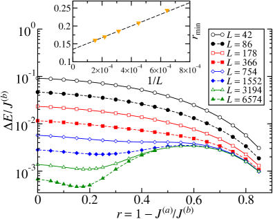
Figure 4: Linear-log plot the energy gap as a function of the coupling modulation $r$ for the Heisenberg chain with couplings following the sequence in Eq. (2) for various chain lengths $L$. The inset shows the position of the relative minimum in the curves for large $L$, using also the intermediate values $L=2226$ and $L=4582$ (not shown for the sake of clarity).

In order to investigate the Heisenberg chain ($\Delta=1$), we performed numerical calculations using the quantum Monte Carlo (QMC) and the density-matrix renormalization group (DMRG) algorithms from the ALPS project(Albuquerque et al., 2007; Bauer et al., 2011).

We employed the DMRG method for calculating the energy gap $\Delta E$ defined as the energy difference between the ground state (with total spin $S_{T}=0$) and the first excited state ($S_{T}=1$), using even lattice sizes ranging from $L=42$ to $6\,574$. Except for the largest chain size, we used up to $50$ warm-up states to grow the DMRG blocks, keeping a maximum of up to $500$ SU(2) states during the (up to 20) sweeps. For $N=6\,574$, we used up to $100$ warm-up sates and $1\,000$ SU(2) states during $30$ sweeps. The modulation strength was varied starting from $r=0$ to $0.85$ and we increased the above simulational parameters from their default values until the energies for each state converged within a relative error below $10^{-8}$. For $r>0.85$ convergence could not be obtained with the maximum values of the above parameters. For the largest system size studied ($N=6\,574$), despite the higher number of states kept, convergence of the gaps was still poorer than for smaller sizes, and we estimate a higher relative error around $10^{-4}$. Figure 4 shows the results of these calculations for various chain lengths. For $r\approx 0$ the finite-size gaps scale as $L^{-z}$ with a (clean) dynamical exponent $z=z_{{\rm clean}}=1$, whereas for larger $r$ they converge to a finite value exhibiting a maximum $\approx 3\times 10^{-3}J^{(b)}$ at $r\approx 0.6$. For large $L$, local minima are visible near $r\approx 0.2$. Their precise positions are obtained from quadratic fits and plotted as a function of $1/L$ in the inset. From a linear extrapolation, we conclude that the minimum occurs at $r_{c}\approx 0.135$ for $L\rightarrow\infty$, therefore supporting the existence of a finite range $0\leq r\leq r_{c}$ for which the system is gapless in the thermodynamic limit. This is in agreement with the simplest scenario of a single critical point and with our perturbative RG predictions. The appearance of a gap only for sufficiently strong modulation is consistent with the emergent dimerization scenario predicted by the SDRG method. A sketch of a generic phase diagram is given in Fig. 1.

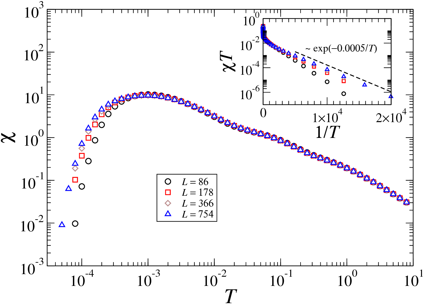
Figure 5: Susceptibility $\chi$ as a function of temperature $T$ for the Heisenberg chain with couplings following the sequence in Eq. (2), for a coupling ratio $J^{\left(a\right)}/J^{\left(b\right)}=1/10$. The results were obtained by using the SSE QMC algorithm, with open chains containing $N\in\left\{86,178,366,754\right\}$ spins. The inset shows that the product $\chi T$ follows $\exp\left(-\Delta E/T\right)$, with a size-dependent energy gap $\Delta E$ which approaches $\approx 5\times 10^{-4}J_{b}$ as $N\rightarrow\infty$. Temperature is measured in units of $J^{\left(b\right)}/k_{B}$. The oscillations in $d\chi/dT$ for temperatures between $T\simeq 10$ and $T\simeq 10^{-3}$ reflect the energy scales associated with the formation of “spin molecules”, as predicted by the SDRG scheme (see main text).

The existence of a gap for strong modulation in the Heisenberg limit is also confirmed by QMC calculations based on the stochastic series expansion (SSE) algorithm(Alet et al., 2005; Albuquerque et al., 2007) with up to $2\times 10^{5}$ thermalization steps and $10^{6}$ sweeps. Figure 5 shows the results of QMC calculations of the magnetic susceptibility $\chi$ for a coupling ratio $J^{\left(a\right)}/J^{\left(b\right)}=1/10$, with open chains containing from $86$ to $754$ spins. At low temperatures, the results conform to the expected behavior

$$\chi\left(T\right)\sim\frac{e^{-\Delta E/T}}{T}$$ (14)

in the presence of an energy gap $\Delta E$. As shown in the inset, the estimated value of the gap ($\approx 5\times 10^{-4}J^{(b)}$) is compatible with those provided by the DMRG calculations. We also performed QMC calculations for $J^{\left(a\right)}/J^{\left(b\right)}=4/10$ and $J^{\left(a\right)}/J^{\left(b\right)}=9/10$ (not shown), again obtaining energy gaps compatible with those provided by DMRG.

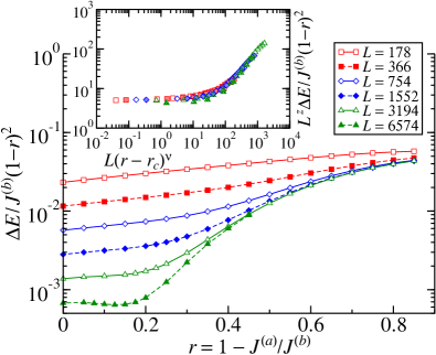
Figure 6: Same data as in Fig. 4 with the energy gap rescaled by $\left(1-r\right)^{2}$. The inset shows the data collapse obtained by the finite-size scaling hypothesis in Eq. (15) using $r>r_{c}=0.135$, $z=1$ and $\nu=2$.

Rescaling the finite-size gaps by the asymptotic dependence $\sim\left(1-r\right)^{2}$ in Eq. (3), a monotonic behavior of the rescaled gaps with $L$ and $r>r_{c}$ becomes manifest, as shown in Fig. 6. It then suggests that a data collapse with a finite-size scaling hypothesis may be possible. For $r>r_{c}$, we expect that in the thermodynamic limit the gap scales as $\Delta E_{\infty}\sim\xi^{-z}\sim\left(r-r_{c}\right)^{z\nu}$, in which $\xi$ is the correlation length, while $z$ and $\nu$ are critical exponents. This gives rise to a finite-size scaling hypothesis

$$\Delta E_{N}=\xi^{-z}F(\xi/L)=L{}^{-z}{\cal F}\left(L\left(r-r_{c}\right)^{\nu}\right),$$ (15)

with scaling functions $F\left(x\right)$ and ${\cal F}\left(x\right)=x^{z}F\left(1/x\right)$.

The plots in the inset of Fig. 6, obtained with $r_{c}=0.135$, $z=z_{{\rm clean}}=1$ and $\nu=2$, show that our DMRG data are compatible with Eq. (15). [Close to the critical point the rescaling of the data by $\left(1-r\right)^{2}$ becomes irrelevant.] This strongly suggests that a true phase transition takes place and that the system is indeed gapless for $r<r_{c}$, in agreement with the perturbative RG prediction.

V Conclusions

We showed that the interplay between strong modulation and interactions induces a transition to a gapped phase in a broad class of deterministic disordered (aperiodic) spin-1/2 chains. In this phase we identify a surprisingly emergent dimerization of the effective low-energy chain, which is quite distinct from any other known gap-inducing mechanism, such as the explicit introduction of dimerization or the spin-Peierls (Majumdar-Ghosh) mechanism related to a spontaneous breaking of translational symmetry via spin-phonon (sufficiently strong frustrating next-nearest-neighbor or, for $S>1/2$, biquadratic) interactions.

Deep inside the aperiodic dimer phase, we showed that the first excited many-body band (corresponding to one-triplon excitations) is entirely localized. Whether these lowest-energy quasiparticle excitations remain localized throughout the entire dimerized phase is a topic left for future research. Another question we leave for future investigation is whether the higher-energy bands also harbor localized states.

Having characterized our zero-temperature phase transition, and in view of the recent evidence that localized ground states correspond to many-body localized excited eigenstates of related Hamiltonians(Dupont and Laflorencie, 2018), we hope our model may be useful to shed light on the nature of the many-body localization transition, which remains largely unclear (Nandkishore and Huse, 2015; Altman and Vosk, 2015).

Our results also apply to interacting fermionic models which are equivalent to the quantum spin chains explicitly discussed here, and in principle could be put to experimental test in the context of cold-atom systems. Along the lines discussed in Ref. Duan et al., 2003, that would involve trapping fermionic atoms in optical lattices. The antiferromagnetic interactions between effective spin degrees of freedom would be related to the atomic tunneling rates between neighboring extrema of the light patterns, and these rates could be made aperiodic by employing several laser sources(Jagannathan and Duneau, 2014), possibly in combination with a cut-and-project construction(Singh et al., 2015). The local intensities at the potential extrema must also be controlled, which could be arranged by employing a digital mirror device(Choi et al., 2016).

Finally, we point out that, in the fermion context, the transition we identified is a metal-insulator transition very distinct from the conventional cases of the Mott and the Anderson transitions. It is driven by both strong interactions and disorder modulation, yielding a fundamentally different insulating phase which has no charge order and exhibits a spectral gap, the first excited band being localized.

Appendix A The Harris–Luck criterion, aperiodic sequences and geometric fluctuations

In order to determine the stability of a clean critical system against the perturbative effects of aperiodicity ($\left|r\right|\ll 1$), Luck(Luck, 1993a) generalized the Harris criterion(Harris, 1974) for the case of deterministic disorder. In the present context, one then quantifies the geometric fluctuations of nonoverlapping letter pairs via the wandering exponent $\omega<1$ defined by

$$G\left(N\right)\equiv\left|N^{\left(aa\right)}-p_{aa}N\right|\sim N^{\omega},$$ (16)

in which $N^{\left(aa\right)}$ denotes the number of $aa$ pairs in the sequence built from cutting the infinite sequence at the $N$th pair, and $p_{aa}$ is the expected fraction of $aa$ pairs in the $N\rightarrow\infty$ limit. Once $\omega$ is determined, the Harris–Luck criterion states that, necessarily, for a clean critical point to be stable against aperiodic weak modulation, the wandering exponent must fulfill

$$\omega<\omega_{c}=\max\left\{0,1-(d\nu)^{-1}\right\},$$ (17)

where $d$ is the number of spatial dimensions in which the system is disordered and $\nu$ is the correlation length critical exponent of the clean theory. As a self-consistent criterion for the stability of the clean fixed point, upon its violation the Harris–Luck criterion does not tells us what is the low-energy physics replacing that of the clean system. We mention that all cases previously studied indicate that the system remains critical but with a larger dynamical exponent(Vieira, 2005a, b).

When fulfilled ($\omega<\omega_{c}$), the Harris–Luck criterion suggests that the corresponding aperiodic sequence is an irrelevant perturbation. Finally, for $\omega=\omega_{c}$ the perturbation is marginal and thus nonuniversal effects may be expected. In this case, a less general approach (as discussed later) is thus required for determining the precise fate of the clean critical point.

We would like to stress the distinction between the strength of the geometric fluctuations, gauged by the wandering exponent $\omega$, and the strength of the aperiodic modulation $r=1-J^{(a)}/J^{(b)}$: for a given $\omega$ (i.e., a given substitution rule) we can tune the system from the clean limit ($r=0$) to the strong-modulation regime ($r\rightarrow 1$ or $r\rightarrow-\infty$). Consider, for concreteness, the pair substitution rule giving rise to the Rudin–Shapiro sequence,

$$\left\{\begin{array}[]{ccc}aa&\rightarrow&aa\,ab\\ ab&\rightarrow&aa\,ba\\ ba&\rightarrow&bb\,ab\\ bb&\rightarrow&bb\,ba\end{array}\right..$$ (18)

The geometric fluctuations of nonoverlapping letter pairs after $n$ iterations of the substitution rule are quantified by

$$G_{n}\equiv\left|N_{n}^{\left(aa\right)}-p_{aa}N_{n}\right|\sim N_{n}^{\omega_{\text{nat}}},$$ (19)

in which $N_{n}$ (called the natural length of the sequence) is the total number of letter pairs obtained after $n$ iterations of the substitution rule, $N_{n}^{\left(\alpha\beta\right)}$ is the corresponding number of $\alpha\beta$ pairs, $p_{\alpha\beta}$ is the expected fraction of $\alpha\beta$ pairs in the $n\rightarrow\infty$ limit, and

$$\omega_{\text{nat}}=\frac{\ln\left|\lambda_{2}\right|}{\ln\lambda_{1}}$$ (20)

is the natural wandering exponent(Luck, 1993b), $\lambda_{1}$ and $\lambda_{2}$ being, respectively, the two largest eigenvalues (in absolute value) of the substitution matrix

$$\mathbb{M}=\left(\begin{array}[]{cccc}\#_{aa}(w_{aa})&\#_{aa}(w_{ab})&\#_{aa}(w_{ba})&\#_{aa}(w_{bb})\\ \#_{ab}(w_{aa})&\#_{ab}(w_{ab})&\#_{ab}(w_{ba})&\#_{ab}(w_{bb})\\ \#_{ba}(w_{aa})&\#_{ba}(w_{ab})&\#_{ba}(w_{ba})&\#_{ba}(w_{bb})\\ \#_{bb}(w_{aa})&\#_{bb}(w_{ab})&\#_{bb}(w_{ba})&\#_{bb}(w_{bb})\end{array}\right),$$ (21)

for which $\#_{\alpha\beta}\left(w_{\gamma\delta}\right)$ denotes the number of $\alpha\beta$ pairs in the word associated with the $\gamma\delta$ pair in the substitution rule. (Notice that $G_{n}$ could equally have been defined in terms of a different $\alpha\beta$ pair, which would not affect the value of $\omega_{\text{nat}}$.)

It is important to notice the difference between the geometrical fluctuations defined in Eqs. (16) and (19). Evidently, $G(N_{n})=G_{n}$. Moreover,

$$\omega\geq\omega_{\text{nat}}.$$ (22)

In order to illustrate the difference, we will compare $G(N)$ and $G_{n}$ for different sequences.

Let us start with the Rudin–Shapiro sequence (18), for which $\omega_{\text{nat}}=\frac{1}{2}$. As plotted in Fig. 7, both geometric fluctuations $G(N)$ and $G_{n}$ scale as $N^{\omega}$ with $\omega=\omega_{\text{nat}}=\frac{1}{2}$. This equality between $\omega_{\text{nat}}$ and $\omega$ can be verified for all the aperiodic sequences generated by substitution rules with $\omega_{\text{nat}}>0$ investigated in Refs. Vieira, 2005a, b.

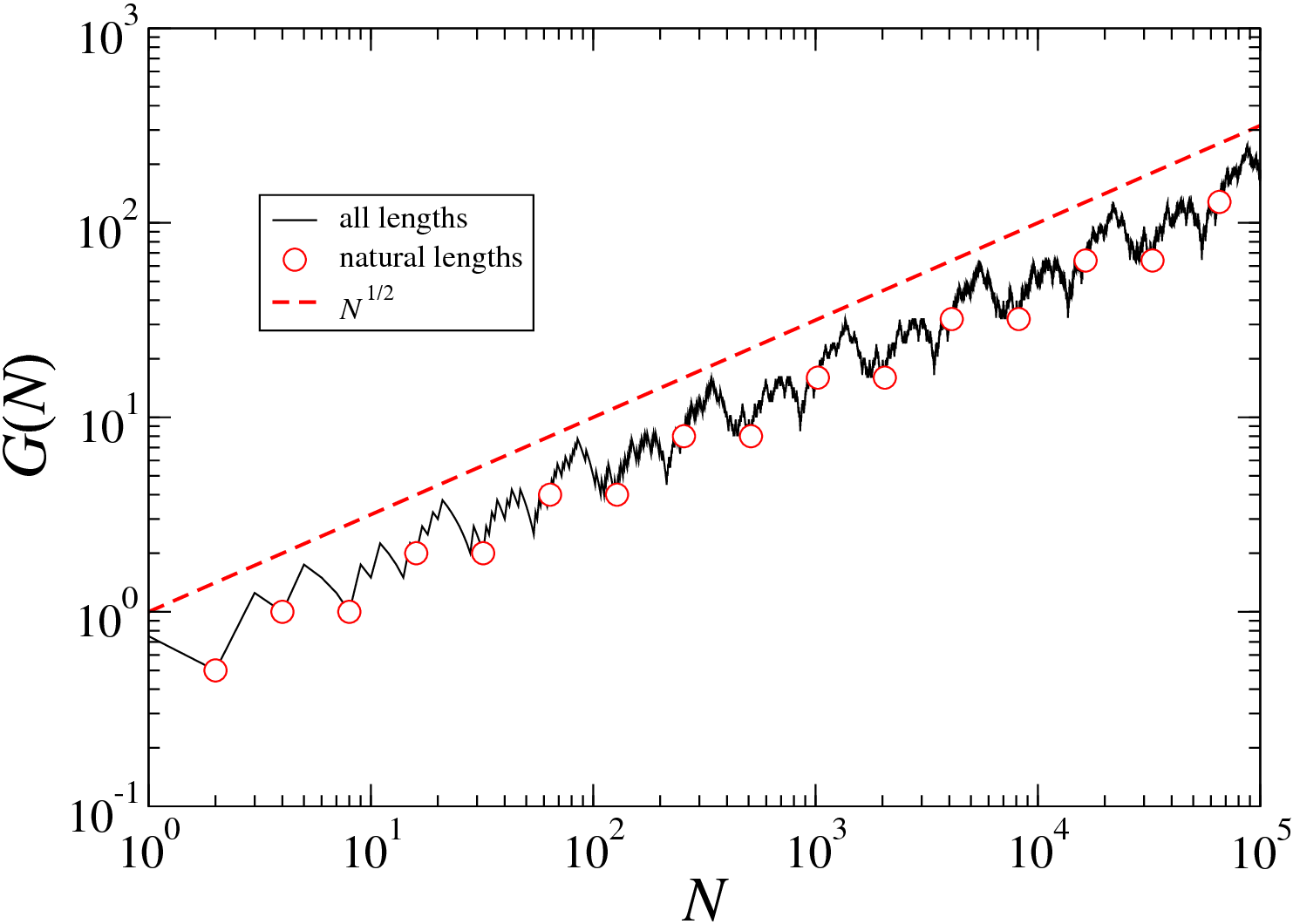
Figure 7: Comparison between geometric fluctuations induced by the Rudin-Shapiro sequence Eq. (18) as calculated for all lengths (solid line) and only for the natural lengths of the sequence (circles). The red dashed line is proportional to $N^{1/2}$. Notice the existence of both stronger and weaker fluctuations in the neighborhood of the natural lengths.

We now turn our attention to the more involved case in which $\omega_{\text{nat}}\leq 0$. One paradigmatic example for $\omega_{\text{nat}}=0$ is the so-called Fibonacci sequence defined (for letter pairs) by the substitution rule

$$\left\{\begin{array}[]{ccc}aa&\rightarrow&ab\,aa\,ba\,ba\,ab\\ ab&\rightarrow&ab\,aa\,ba\,ba\\ ba&\rightarrow&ab\,aa\,ba\,ab\end{array}\right..$$ (23)

In this case, as shown in Fig. 8, the strong fluctuations of $G(N)$ are unbounded but only grow logarithmically. In this case, it is desirable to distinguish a logarithmic growth, as for $G(N)$, from a constant, as for $G_{n}$. Here, we will simply define the wandering exponent as $\omega=0^{+}$, which is still compatible with Eq. (22).

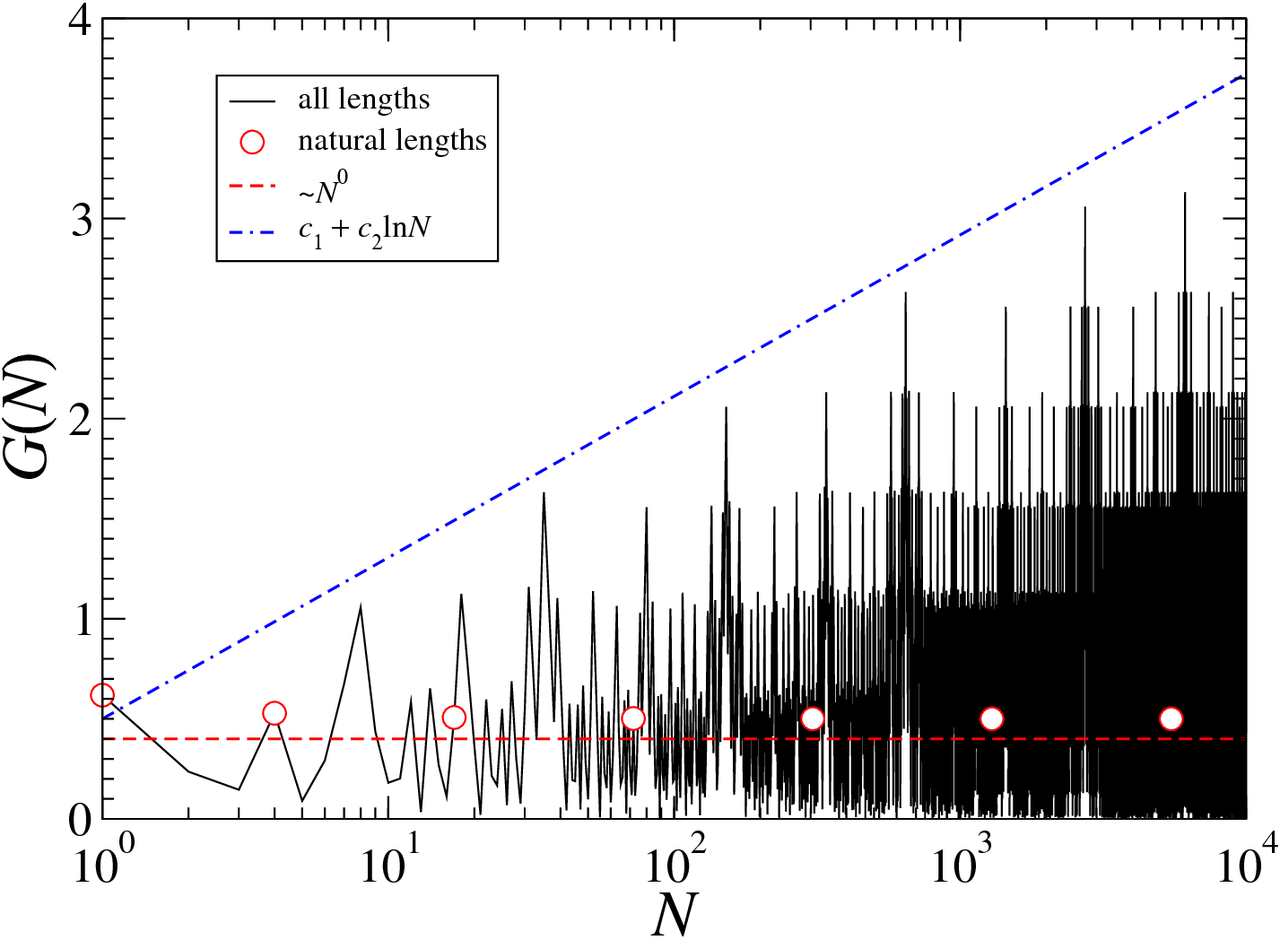
Figure 8: Comparison between geometric fluctuations induced by the Fibonacci sequence (23) as calculated for all lengths (solid line) and only for the natural lengths of the sequence (circles). The red dashed red line is proportional to $N^{0}$. Notice that the stronger fluctuations scale at most logarithmically with $N$ (blue dot-dashed line, with $c_{1}$ and $c_{2}$ constants of order 1).

The sequences for which $\omega_{\text{nat}}<0$ (and finite), as those of interest in this work, are said to exhibit the Pisot property (Godrèche and Luck, 1992), giving rise to bounded fluctuations as $N\rightarrow\infty$. Let us illustrate this case with the sequence defined by the substitution rule in Eq. (2). The corresponding natural wandering exponent $\omega_{\text{nat}}=-1$ obtained from Eq. (20) is in agreement with the observed one shown in Fig. 9. In addition, notice that the strongest fluctuations (corresponding to lengths other than the natural ones) are also bounded. For this reason, we define the wandering exponent as $\omega=0^{-}$.

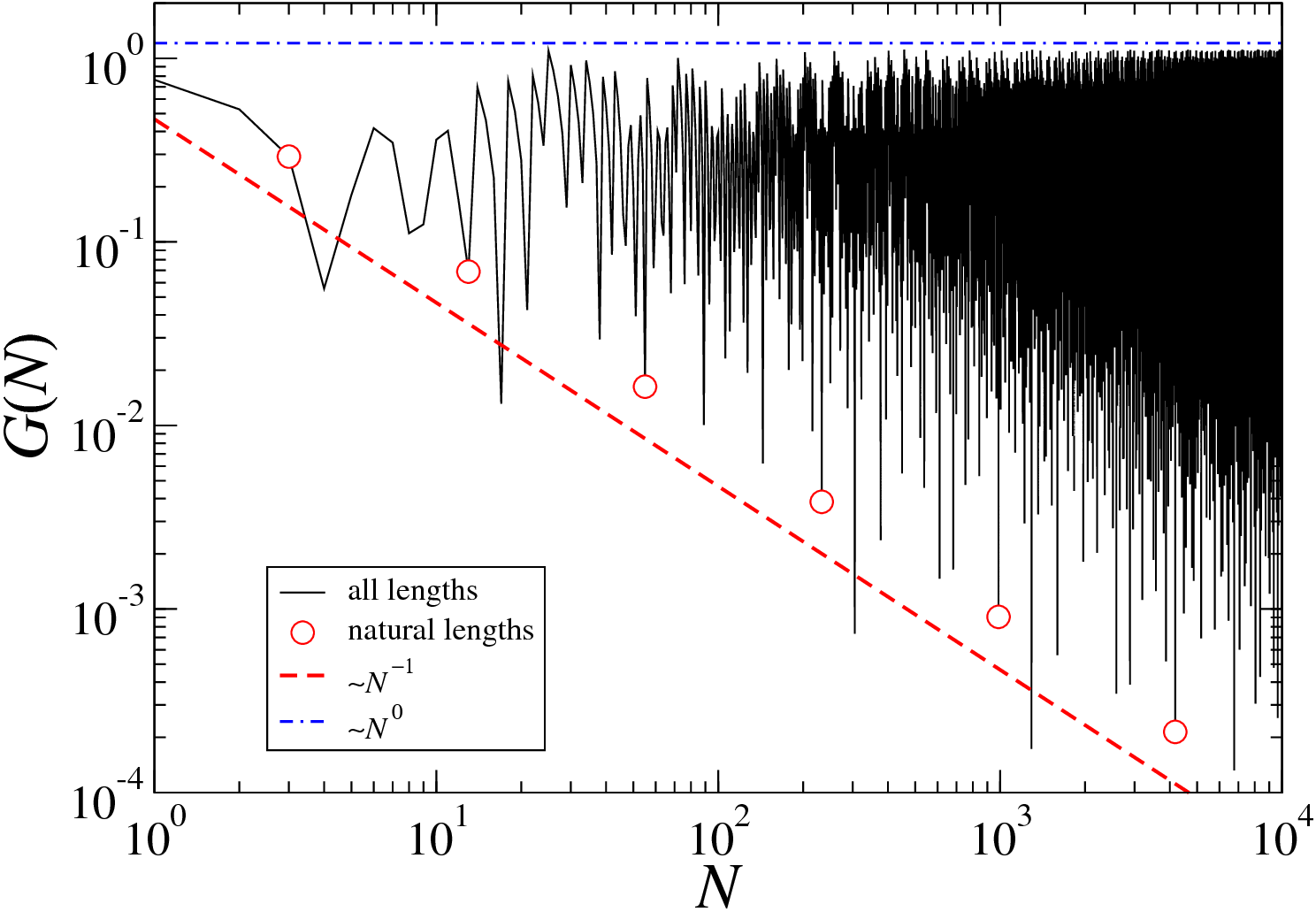
Figure 9: Comparison between geometric fluctuations induced by the sequence in Eq. (2) as calculated for all lengths (solid line) and only for the natural lengths of the sequence (circles). The red dashed curve is proportional to $N^{-1}$. Notice that the stronger fluctuations scale as $N^{0}$ for large $N$.

We would like to point out that, for our numerical analysis of the sequence in Eq. (2) of the main text, we used chains with lengths not restricted to the natural ones. In other words, the striking features we observed (as the gap behavior in Fig. 3 of the main text) are not an artifact of choosing special chain lengths.

Finally, we mention the existence of many other sequences sharing the same features of the sequence (2), also yielding the same emergent dimerization phenomena in the nonperturbative regime, as reported in the main text. The sequences are such that $\omega=0^{-}>\omega_{\text{nat}}>-\infty$, and do not induce an average dimerization. A simple way to construct such a sequence is via small tweaks of the sequence in (2), as for example

$$\left\{\begin{array}[]{ccc}aa&\rightarrow&aa\,ab\,ba\\ ab&\rightarrow&aa\,ba\,ab\,aa\\ ba&\rightarrow&aa\,ab\,ba\end{array}\right.,$$ (24)

which also yields $\omega_{\text{nat}}=-1$. Other examples are the sequence

$$\left\{\begin{array}[]{ccc}aa&\rightarrow&aa\,ab\,aa\,ba\\ ab&\rightarrow&ba\,ab\\ ba&\rightarrow&aa\,ba\,aa\,ab\end{array}\right.,$$ (25)

for which $\omega_{\text{nat}}=\frac{\ln\left(2-\sqrt{2}\right)}{\ln\left(2+\sqrt{2}\right)}\approx-0.44$, and the sequence generated by the substitution rule

$$\left\{\begin{array}[]{ccc}aa&\rightarrow&aa\,ba\,ab\,ab\,ba\\ ab&\rightarrow&aa\,ab\,ba\\ ba&\rightarrow&aa\,ab\,aa\,ba\,ba\,ab\end{array}\right.,$$ (26)

for which $\omega_{\text{nat}}=\frac{\ln\left|2-\sqrt{7}\right|}{\ln\left(2+\sqrt{7}\right)}\approx-0.28.$ Somewhat simpler sequences are given by the substitution rules

$$\left\{\begin{array}[]{ccc}aa&\rightarrow&aa\,ab\,ba\\ ab&\rightarrow&aa\,aa\\ ba&\rightarrow&ba\,ab\,aa\end{array}\right.,$$ (27)

for which $\omega_{\text{nat}}=\frac{\ln\left|1-\sqrt{3}\right|}{\ln\left(1+\sqrt{3}\right)}\approx-0.310$, and

$$\left\{\begin{array}[]{ccc}aa&\rightarrow&aa\,ab\,ba\\ ab&\rightarrow&aa\\ ba&\rightarrow&ba\,ab\,aa\end{array}\right.,$$ (28)

for which $\omega_{\text{nat}}=-1$.

In order to obtain other similar sequences, one can start from a trial substitution matrix for 3 letter pairs ($aa$, $ab$, and $ba$), and calculate its largest eigenvalue, the corresponding (right) eigenvector, and $\omega_{\text{nat}}$. The desired sequences are those with $-\infty<\omega_{\text{nat}}<0$, yielding $\omega=0^{-}$, and having equal second and third components of the eigenvector associated with the largest eigenvalue, which ensures that there is no average dimerization. (The components of this eigenvector are proportional to the fraction of the corresponding pairs in the infinite sequence.)

Appendix B Perturbative renormalization group for the antiferromagnetic XXZ chain

The renormalization-group (RG) equations obtained from the perturbative approach of Vidal, Mouhanna and Giamarchi(Vidal et al., 1999, 2001) are

$$\frac{dK}{dl}=-K^{2}\Xi\left(l\right),$$ (29)

$$\frac{dy_{Q}}{dl}=\left(2-K\right)y_{Q},$$ (30)

with

$$\Xi\left(l\right)=\frac{1}{2}\sum_{Q}y_{Q}^{2}\left[R\left(Q^{+}a\left(l\right)\right)+R\left(Q^{-}a\left(l\right)\right)\right],$$ (31)

where $Q^{\pm}=Q\pm\pi$, the $y_{Q}=\lambda a\left|\tilde{J}\left(Q\right)\right|/u$ are initially the dimensionless Fourier components of the bonds $J_{i}$, $\lambda$ measures the modulation strength and $l$ is a scaling factor defined by $a\left(l\right)=a_{0}e^{l}$, the constant $a_{0}$ being proportional to the original lattice spacing. (Without loss of generality, we take $a_{0}=1$.) $R\left(x\right)$ is a cutoff function used to eliminate short-length degrees of freedom. We used for $R\left(x\right)$ the precise form

$$R\left(x\right)=\frac{1}{1+x^{4}},$$ (32)

but other functions having appreciable values only for $\left|x\right|<1$ yield similar results. The Luttinger parameter $K$ has an initial value which varies with the anisotropy $\Delta$ of the XXZ chain according to(Luther and Peschel, 1975; Kossow et al., 2012)

$$K=\left[2-\frac{2}{\pi}\arccos\left(\Delta\right)\right]^{-1},$$ (33)

therefore ranging from $K=2$ (for $\Delta=-\frac{1}{\sqrt{2}}$), to $K=\frac{3}{2}$ (for $\Delta=-\frac{1}{2}$), to $K=1$ (for $\Delta=0$, corresponding to the XX chain), and finally to $K=\frac{1}{2}$ (for $\Delta=1$, corresponding to the Heisenberg chain). The correlation-length critical exponent of the underlying dimerization transition is related to $K$ by

$$\nu=\frac{1}{2-K}.$$ (34)

Finally, the remaining Luttinger parameter, $u$, which appears in the definition of $y_{Q}$, has the initial value

$$u=\frac{2K}{2K-1}\sin\left[\pi\left(1-\frac{1}{2K}\right)\right],$$ (35)

corresponding to the velocity of the excitations, and its renormalization is neglected since it only gives rise to higher order corrections(Vidal et al., 2001).

For a dimerized chain, in which the bonds alternate between $J_{2i}=J+\lambda/2$ and $J_{2i+1}=J-\lambda/2$, we have $\hat{J}\left(Q\right)\propto\delta\left(Q-\pi\right)$, so we only have to worry about the renormalization of $y_{\pi}$, whose bare value for a large chain with $N$ sites is proportional to $N$. Starting from $K<2$, since $R\left(Q^{-}\alpha\left(l\right)\right)=R\left(0\right)=1$ for all $l$, it is clear that $K$ flows toward $0$, the strong-coupling regime where the perturbative RG method is no longer valid. This is consistent with the fact that dimerization opens an excitation gap in the anisotropy regime $-\frac{1}{\sqrt{2}}<\Delta\leq 1$ which contains both the XX and the Heisenberg chains. Notice that in general a nonzero $y_{\pi}$, even if other Fourier weights are also nonzero, trivially leads to a runaway flow to the strong-coupling limit, with the opening of a gap; such cases are associated with the presence of average dimerization. In this paper we only deal with the cases for which $y_{\pi}=0$.

Consider the case in which spins interact through nearest-neighbor bonds $\left\{J_{i}\right\}$ taking values $J^{\left(a\right)}$ and $J^{\left(b\right)}$ according to the sequence of letters $a$ and $b$ obtained by iterating the substitution rule in Eq. (2). As it leads to $\omega=0^{-}$, we expect from the Harris–Luck criterion that weak aperiodicity is irrelevant.

Indeed, it turns out that the numerical solution of the perturbative RG equations for any finite approximant to the infinite sequence leads to a flow in which the asymptotic value of $K$ remains close to the initial value for all $\frac{1}{2}<K<2$, pointing to the irrelevance of weak aperiodic modulation for the easy-plane antiferromagnetic XXZ chain. This is related to the fact that $\tilde{J}\left(Q\right)$, which exhibits the self-similar structure characteristic of aperiodic sequences, has no peaks at nor in a finite neighborhood of $Q=\pi$, as further discussed below.

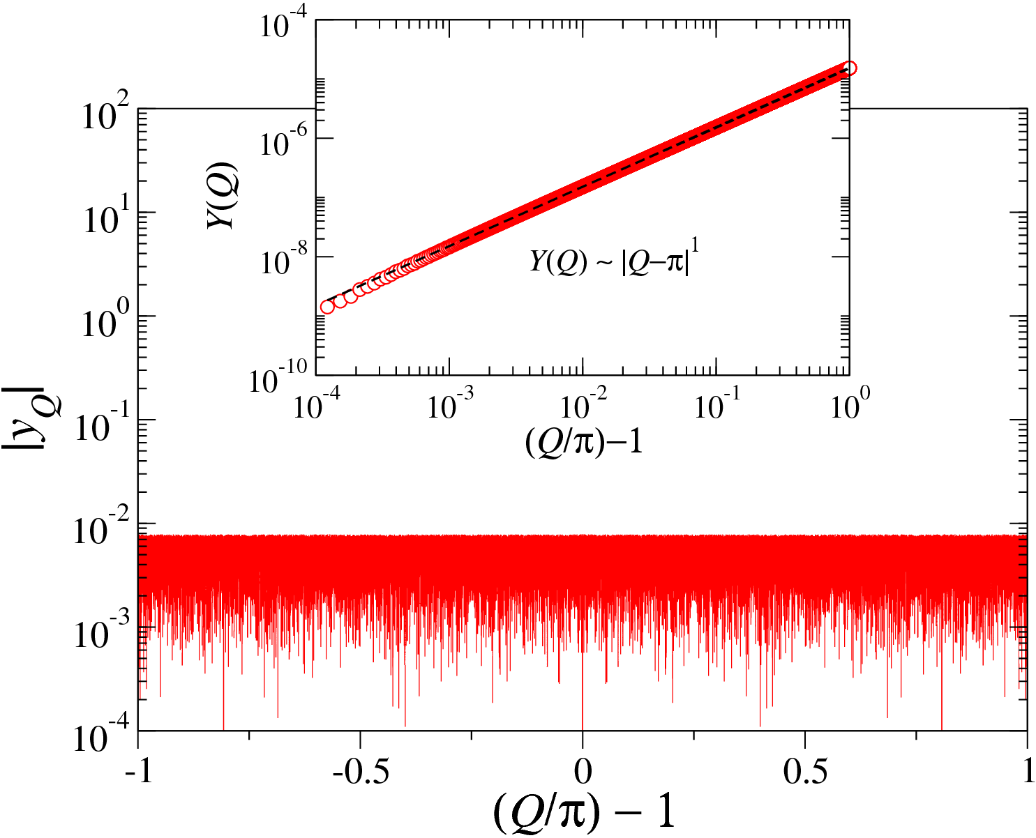
Figure 10: Fourier spectrum of the Rudin–Shapiro sequence. The inset shows $Y\left(Q\right)=\sum_{q=\pi}^{Q}y^{2}\left(q\right)$, which behaves as $\left|Q-\pi\right|^{2\alpha+1}$ if $y\left(Q\right)\sim\left|Q-\pi\right|^{\alpha}$.

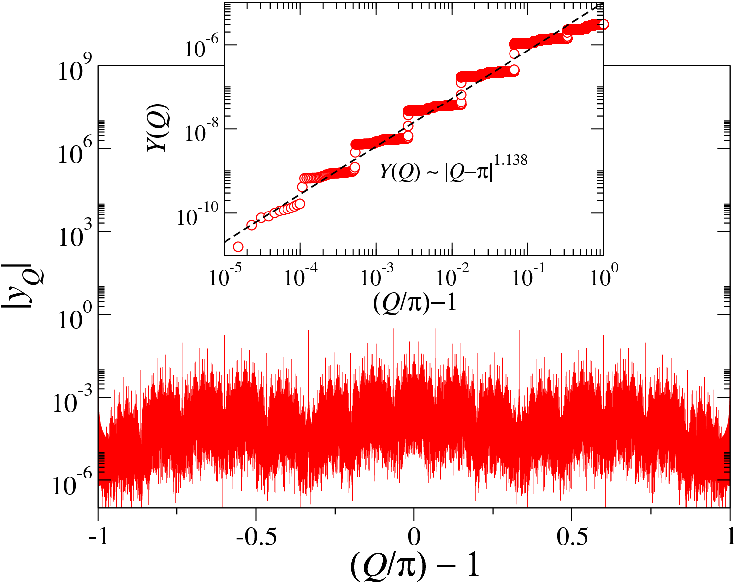
Figure 11: Fourier spectrum of the 6-3 sequence. The inset shows $Y\left(Q\right)=\sum_{q=\pi}^{Q}y^{2}\left(q\right)$, which behaves as $\left|Q-\pi\right|^{2\alpha+1}$ if $y\left(Q\right)\sim\left|Q-\pi\right|^{\alpha}$.

In contrast, the same approach applied to the Rudin–Shapiro sequence (18) (for which $\omega=\frac{1}{2}$), points to its relevance in the same anisotropy regime. The same behavior is observed for the fivefold-symmetry sequence ($\omega\approx 0.285$) and the 6-3 sequence ($\omega\approx 0.431$) investigated in Ref. Vieira, 2005b. In all three cases, although $y_{\pi}=0$, indicating that there is no average dimerization, the Fourier spectra are self-similar, with peaks behaving in the neighborhood of $Q=\pi$ as $\left|Q-\pi\right|^{\alpha}$, the constant $\alpha$ depending on the sequence, as illustrated in Figs. 10 and 11.

This last observation allows us to attempt an approximate solution of the perturbative RG equations. The reasoning is as follows(Vidal et al., 2001). Let us assume that $K$ varies much less than $y_{Q}$ with $l$, so that we can write

$$y_{Q}\left(l\right)\simeq y_{Q}\left(0\right)e^{\left(2-K\right)l},$$ (36)

in which $y_{Q}\left(0\right)$ corresponds to the Fourier spectrum of the original bonds. In this case, the scaling behavior of $\Xi\left(l\right)$ is given by

$$\Xi\left(l\right)\simeq e^{-\left(4-2K\right)l}\sum_{Q\in\mathcal{S}\left(l\right)}y_{Q}^{2}\left(0\right),$$ (37)

where $\mathcal{S}\left(l\right)$ is the set of wavevectors, defined by $\mathcal{S}\left(l\right)=\left\{Q\left|\left|Q-\pi\right|\leq e^{-l}\right.\right\}$, for which the cutoff function $R\left(Q^{-}e^{l}\right)$ is non-negligible. Using $y_{Q}^{2}\left(0\right)\sim\left|Q-\pi\right|^{2\alpha}$, we thus obtain

$$\sum_{Q\in\mathcal{S}\left(l\right)}y_{Q}^{2}\left(0\right)\sim\int_{0}^{e^{-l}}x^{2\alpha}dx\sim e^{-\left(2\alpha+1\right)l},$$ (38)

so that

$$\Xi\left(l\right)\sim e^{-\left(3-2K-2\alpha\right)l}.$$ (39)

From Eq. (29) we see that the flow of the Luttinger parameter $K$ crucially depends on the scaling behavior of $\Xi\left(l\right)$. If $\Xi\left(l\right)>1$ then $K$ flows to the strong-coupling limit where the perturbative treatment breaks down, and aperiodicity is predicted to be relevant. On the other hand, if $\Xi\left(l\right)<1$, the flow stops at some $\lambda$-dependent finite value, and aperiodicity is predicted to be irrelevant. For a given sequence (i.e. a given $\alpha$), there is a critical value of $K$ separating these two regimes:

$$K_{c}=\frac{3}{2}-\alpha.$$ (40)

For $K<K_{c}$ we expect weak aperiodic modulation to be relevant.

However, Eq. (34), along with the critical condition $\nu_{c}=\left(1-\omega\right)^{-1}$ derived from the Harris–Luck criterion, also implies the existence of a critical value $K_{c}$ of the Luttinger parameter $K$, but in terms of the wandering exponent,

$$K_{c}=1+\omega.$$ (41)

Using this last equation, derived from the Harris–Luck criterion for the aperiodic XXZ chain, we can relate the Fourier-spectrum exponent $\alpha$ and the pair wandering exponent $\omega$ through

$$\omega=\frac{1}{2}-\alpha.$$ (42)

The values of $\alpha$ obtained by fitting the integrated Fourier spectra of the Rudin–Shapiro, fivefold-symmetry and 6-3 sequences shown in Figs. 10 and 11 are fully consistent with Eq. (42). The relation in Eq. (42) is also consistent with a result indicating that aperiodic fluctuations in tight-binding Hamiltonians (equivalent to XX chains) are relevant if, in our notation, $\alpha<\frac{1}{2}$, which corresponds to $\omega>0$; see Ref. Luck, 1989.

For the Fibonacci sequence, whose wandering exponent is $\omega=0^{+}$, the relevance of weak modulation was predicted via the perturbative renormalization-group approach in Refs. Vidal et al., 1999, 2001; Hida, 2001. It is possible to check that the Fourier spectrum of the Fibonacci sequence yields $\alpha=\frac{1}{2}$, again in agreement with Eq. (42).

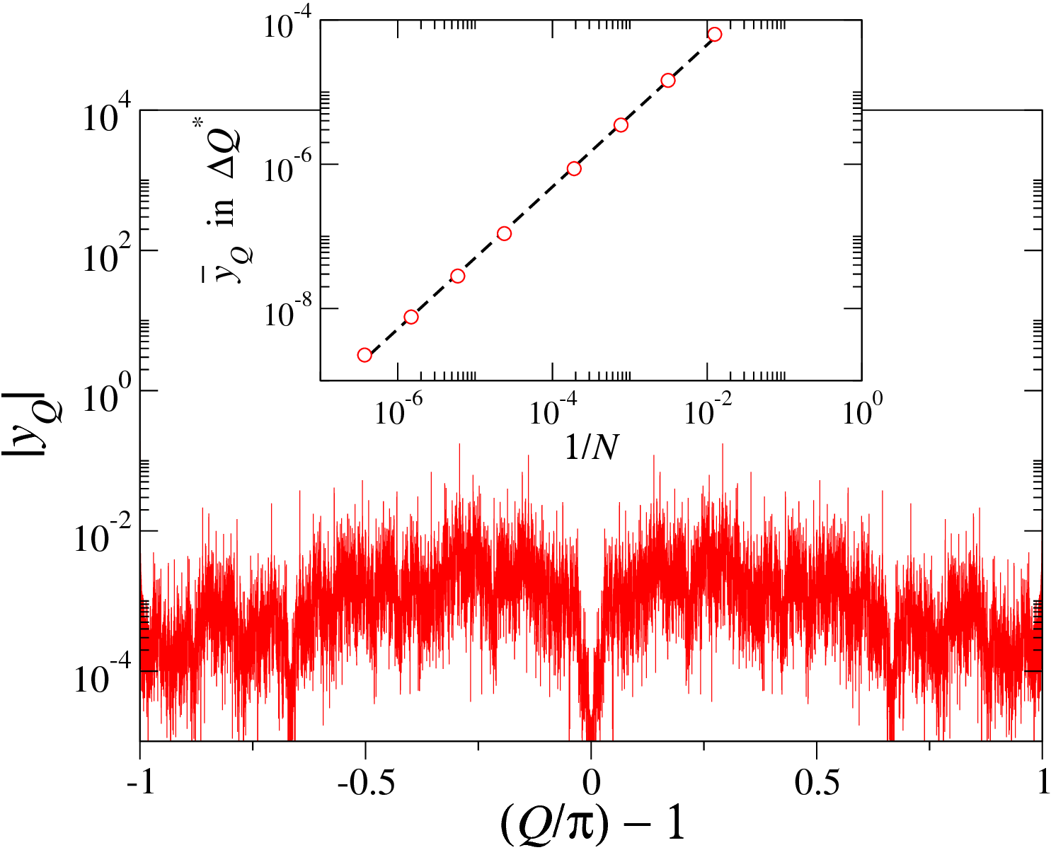
Figure 12: Fourier spectrum of the sequence in Eq. (26). The inset shows the finite-size scaling behavior of the average value of the Fourier weights in a region of width $\Delta Q^{*}=10^{-3}\pi$ around $Q=\pi$.

However, the situation is different for sequences with $\omega=0^{-}$, as those in Eq. (2) and Eqs. (24)–(28). In this case, the Fourier spectrum has a very small and essentially constant weight in a neighborhood of $Q=\pi$ of width $\Delta Q^{*}$ (see Fig. 12). A finite-size analysis indicates that the weight in this region scales with the system size $N$ as $1/N$, and thus vanishes in the thermodynamic limit $N\rightarrow\infty$. This means that the perturbative RG flow stops at a length scale $l^{*}$ for which $e^{-l^{*}}\sim\Delta Q^{*}$. In the weak modulation limit of $\lambda\rightarrow 0$, this length scale is always reached before any relevant flow happens, preserving the initial values of the Luttinger parameters. Therefore, weak aperiodic bond modulation following Eqs. (2) or Eqs. (24)–(28) is irrelevant for the easy-plane antiferromagnetic XXZ chain, as predicted by the Harris–Luck criterion. Moreover, Eq. (42) is no longer verified, as the behavior of the Fourier spectrum around $Q=\pi$ is not compatible with the implied value $\alpha=\frac{1}{2}$.

Appendix C The strong-disorder renormalization group (SDRG)

We consider the results of a numerical implementation of the SDRG approach when couplings are chosen according to the sequence in Eq. (2). As mentioned in the main text, close to the Heisenberg limit this leads to a low-energy effective chain with emergent dimerization, corresponding to an alternating pattern of strong and weak effective couplings. Within the SDRG approach, the strong effective couplings are, suprisingly, all equal and predicted to scale as $\left(J^{\left(a\right)}\right)^{2}/J^{\left(b\right)}$. We now investigate the relation between the magnititude $J$ and length $l$ of the weak effective couplings, as plotted in Fig. 13 for the Heisenberg case ($\Delta=1$) and $r=0.9$. The relation can be well fitted by

$$J\sim e^{-\mu\ln^{2}\left(l/l_{0}\right)},$$ (43)

in which $\mu$ and $l_{0}$ are constants. (Notice only four different lengths were generated for this sequence. Other sequences may have a different number of distinct weak effective couplings.) This form is the same obtained for the Heisenberg chain with couplings following the Fibonacci sequence(Vieira, 2005a, b), for which the pair wandering exponent is $\omega=0^{+}$ but no alternating-coupling pattern is observed.

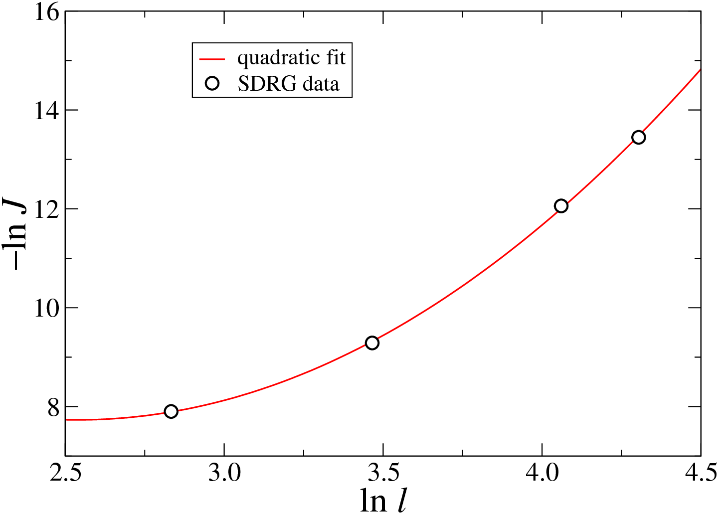
Figure 13: Relation between the strengths $J$ and the lengths $l$ of the weak effective bonds corresponding to the low-energy effective chain when couplings follow the aperiodic sequence in Eq. (2). The continuous line is a fit using Eq. (43). The coupling ratio corresponds to $r=J_{a}/J_{b}=1/10$, and the strengths are given in units of $J_{b}$. For this coupling ratio, the strength of the strong effective bonds, as predicted by the SDRG approach, is $\approx 1.5\times 10^{-3}$, with a length of 10 lattice parameters.

Similar results are also obtained from the SDRG approach for the sequences (24)—(28).

References

- Anderson (1958) P. W. Anderson, “Absence of diffusion in certain random lattices,” Phys. Rev. 109, 1492 (1958).
- Aubry and André (1980) S. Aubry and G. André, “Analyticity breaking and Anderson localization in incommensurate lattices,” Ann. Israel Phys. Soc. 3, 133 (1980).
- Basko et al. (2006) D. M. Basko, I. L. Aleiner, and B. L. Altshuler, “Metal-insulator transition in a weakly interacting many-electron system with localized single-particle states,” Annals of Physics 321, 1126 (2006).
- Nandkishore and Huse (2015) Rahul Nandkishore and David A. Huse, “Many-body localization and thermalization in quantum statistical mechanics,” Annu. Rev. Condens. Matter Phys. 6, 15 (2015).
- Altman and Vosk (2015) E. Altman and R. Vosk, “Universal dynamics and renormalization in many-body-localized systems,” Annu. Rev. Condens. Matter Phys. 6, 383 (2015).
- Iyer et al. (2013) S. Iyer, V. Oganesyan, G. Refael, and D. A. Huse, “Many-body localization in a quasiperiodic system,” Phys. Rev. B 87, 134202 (2013).
- Nag and Garg (2017) S. Nag and A. Garg, “Many-body mobility edges in a one-dimensional system of interacting fermions,” Phys. Rev. B 96, 060203 (2017).
- Khemani et al. (2017) V. Khemani, D. N. Sheng, and D. A. Huse, “Two universality classes for the many-body localization transition,” Phys. Rev. Lett. 119, 075702 (2017).
- Lee et al. (2017) M. Lee, T. R. Look, S. P. Lim, and D. N. Sheng, “Many-body localization in spin chain systems with quasiperiodic fields,” Phys. Rev. B 96, 075146 (2017).
- Roati et al. (2008) G. Roati, C. D’Errico, L. Fallani, M. Fattori, C. Fort, M. Zaccanti, G. Modugno, M. Modugno, and M. Inguscio, “Anderson localization of a non-interacting Bose-Einstein condensate,” Nature 453, 895 (2008).
- Schreiber et al. (2015) M. Schreiber, S. S. Hodgman, P. Bordia, H. P. Lüschen, M. H. Fischer, R. Vosk, E. Altman, U. Schneider, and I. Bloch, “Observation of many-body localization of interacting fermions in a quasirandom optical lattice,” Science 349, 842 (2015).
- Lüschen et al. (2017) H. P. Lüschen, P. Bordia, S. Scherg, F. Alet, E. Altman, U. Schneider, and I. Bloch, “Observation of slow dynamics near the many-body localization transition in one-dimensional quasiperiodic systems,” Phys. Rev. Lett. 119, 260401 (2017).
- Bordia et al. (2017) P. Bordia, H. Lüschen, U. Schneider, M. Knap, and I. Bloch, “Periodically driving a many-body localized quantum system,” Nature Physics 13, 460 (2017).
- Luther and Peschel (1975) A. Luther and I. Peschel, “Calculation of critical exponents in two dimensions from quantum field theory in one dimension,” Phys. Rev. B 12, 3908 (1975).
- Kossow et al. (2012) M. Kossow, P. Schupp, and S. Kettemann, “Critical exponents for antiferromagnetic spin chains obtained from bosonisation,” Int. J. Mod. Phys.: Conf. Series 11, 183 (2012).
- Harris (1974) A. B. Harris, “Effect of random defects on the critical behaviour of Ising models,” J. Phys. C: Solid State Phys. 7, 1671 (1974).
- Doty and Fisher (1992) C. A. Doty and D. S. Fisher, “Effects of quenched disorder on spin-1/2 quantum XXZ chains,” Phys. Rev. B 45, 2167 (1992).
- Fisher (1994) D. S. Fisher, “Random antiferromagnetic quantum spin chains,” Phys. Rev. B 50, 3799 (1994).
- Hoyos et al. (2007) J. A. Hoyos, A. P. Vieira, N. Laflorencie, and E. Miranda, “Correlation amplitude and entanglement entropy in random spin chains,” Phys. Rev. B 76, 174425 (2007).
- Rieger and Iglói (1999) H. Rieger and F. Iglói, “Random quantum magnets with long-range correlated disorder: Enhancement of critical and Griffiths-McCoy singularities,” Phys. Rev. Lett. 83, 3741 (1999).
- Hoyos et al. (2011) J. A. Hoyos, N. Laflorencie, A. P. Vieira, and T. Vojta, “Protecting clean critical points by local disorder correlations,” EPL 93, 30004 (2011).
- Getelina et al. (2016) J. C. Getelina, F. C. Alcaraz, and J. A. Hoyos, “Entanglement properties of correlated random spin chains and similarities with conformally invariant systems,” Phys. Rev. B 93, 045136 (2016).
- Vieira (2005a) A. P. Vieira, “Low-energy properties of aperiodic quantum spin chains,” Phys. Rev. Lett. 94, 077201 (2005a).
- Vieira (2005b) A. P. Vieira, “Aperiodic quantum XXZ chains: renormalization-group results,” Phys. Rev. B 71, 134408 (2005b).
- Vidal et al. (1999) J. Vidal, D. Mouhanna, and T. Giamarchi, “Correlated fermions in a one-dimensional quasiperiodic potential,” Phys. Rev. Lett. 83, 3908 (1999).
- Vidal et al. (2001) J. Vidal, D. Mouhanna, and T. Giamarchi, “Interacting fermions in self-similar potentials,” Phys. Rev. B 65, 014201 (2001).
- Hida (2001) K. Hida, “Quasiperiodic Hubbard Chains,” Phys. Rev. Lett. 86, 1331 (2001).
- Luck (1993a) J. M. Luck, “A Classification of Critical Phenomena on Quasi-Crystals and Other Aperiodic Structures,” EPL 24, 359 (1993a).
- Ma et al. (1979) S.-K. Ma, C. Dasgupta, and C.-K. Hu, “Random antiferromagnetic chain,” Phys. Rev. Lett. 43, 1434 (1979).
- Bhatt and Lee (1982) R. N. Bhatt and P. A. Lee, “Scaling Studies of Highly Disordered Spin- Antiferromagnetic Systems,” Phys. Rev. Lett. 48, 344 (1982).
- Casa Grande et al. (2014) H. L. Casa Grande, N. Laflorencie, F. Alet, and A. P. Vieira, “Analytical and numerical studies of disordered spin-1 Heisenberg chains with aperiodic couplings,” Phys. Rev. B 89, 134408 (2014).
- Oliveira Filho et al. (2012) F. J. Oliveira Filho, M. S. Faria, and A. P. Vieira, “Strong-disorder renormalization group study of aperiodic quantum Ising chains,” J. Stat. Mech. 2012, P03007 (2012).
- Barghathi et al. (2014) H. Barghathi, D. Nozadze, and T. Vojta, “Contact process on generalized Fibonacci chains: Infinite-modulation criticality and double-log periodic oscillations,” Phys. Rev. E 89, 012112 (2014).
- Iglói et al. (2007) F. Iglói, R. Juhász, and Z. Zimborás, “Entanglement entropy of aperiodic quantum spins chains,” EPL 79, 37001 (2007).
- Juhász and Zimborás (2007) R. Juhász and Z. Zimborás, “Entanglement entropy of aperiodic singlet phases,” J. Stat. Mech. 2007, P04004 (2007).
- Javan Mard et al. (2014) H. Javan Mard, José A. Hoyos, E. Miranda, and V. Dobrosavljević, “Strong-disorder renormalization-group study of the one-dimensional tight-binding model,” Phys. Rev. B 90, 125141 (2014).
- Eggarter and Riedinger (1978) T. P. Eggarter and R. Riedinger, Phys. Rev. B 18, 569 (1978).
- Lieb et al. (1961) E. Lieb, T. Schultz, and D. Mattis, “Two soluble models of an antiferromagnetic chain,” Annals of Physics 16, 407 (1961).
- Albuquerque et al. (2007) A. F. Albuquerque, F. Alet, P. Corboz, P. Dayal, A. Feiguin, S. Fuchs, L. Gamper, E. Gull, S. Gürtler, A. Honecker, R. Igarashi, M. Körner, A. Kozhevnikov, A. Läuchli, S. R. Manmana, M. Matsumoto, I. P. McCulloch, F. Michel, R. M. Noack, G. Pawłowski, L. Pollet, T. Pruschke, U. Schollwöck, S. Todo, S. Trebst, M. Troyer, P. Werner, and S. Wessel, “The ALPS project release 1.3: Open-source software for strongly correlated systems,” J. Magn. Magn. Mater. 310, 1187 (2007).
- Bauer et al. (2011) B. Bauer, L. D. Carr, H. G. Evertz, A. Feiguin, J. Freire, S. Fuchs, L. Gamper, J. Gukelberger, E. Gull, S. Guertler, A. Hehn, R. Igarashi, S. V. Isakov, D. Koop, P. N. Ma, P. Mates, H. Matsuo, O. Parcollet, G. Pawlowski, J. D. Picon, L. Pollet, E. Santos, V. W. Scarola, U. Schollwöck, C. Silva, B. Surer, S. Todo, S. Trebst, M. Troyer, M. L. Wall, P. Werner, and S. Wessel, “The ALPS project release 2.0: open source software for strongly correlated systems,” J. Stat. Mech. 2011, P05001 (2011).
- Alet et al. (2005) F. Alet, S. Wessel, and M. Troyer, “Generalized directed loop method for quantum Monte Carlo simulations,” Phys. Rev. E 71, 036706 (2005).
- Dupont and Laflorencie (2018) M. Dupont and N. Laflorencie, “Many-body localization as a large family of localized groundstates,” (2018), arXiv:1807.01313 .
- Duan et al. (2003) L.-M. Duan, E. Demler, and M. D. Lukin, “Controlling spin exchange interactions of ultracold atoms in optical lattices,” Phys. Rev. Lett. 91, 090402 (2003).
- Jagannathan and Duneau (2014) A. Jagannathan and M. Duneau, “Tight-binding models in a quasiperiodic optical lattice,” Acta Phys. Pol. A 126, 490 (2014).
- Singh et al. (2015) K. Singh, K. Saha, S. A. Parameswaran, and D. M. Weld, “Fibonacci optical lattices for tunable quantum quasicrystals,” Phys. Rev. A 92, 063426 (2015).
- Choi et al. (2016) J.-y. Choi, S. Hild, J. Zeiher, P. Schauß, A. Rubio-Abadal, T. Yefsah, V. Khemani, D. A. Huse, I. Bloch, and C. Gross, “Exploring the many-body localization transition in two dimensions,” Science 352, 1547 (2016).
- Luck (1993b) J. M. Luck, “Critical behavior of the aperiodic quantum Ising chain in a transverse magnetic field,” J. Stat. Phys. 72, 417 (1993b).
- Godrèche and Luck (1992) C. Godrèche and J. M. Luck, “Indexing the diffraction spectrum of a non-Pisot self-similar structure,” Phys. Rev. B 45, 176 (1992).
- Luck (1989) J. M. Luck, “Cantor spectra and scaling of gap widths in deterministic aperiodic systems,” Phys. Rev. B 39, 5834 (1989).