Recognizing Visibility Graphs of Polygons with Holes and Internal-External Visibility Graphs of Polygons

Abstract

Visibility graph of a polygon corresponds to its internal diagonals and boundary edges. For each vertex on the boundary of the polygon, we have a vertex in this graph and if two vertices of the polygon see each other there is an edge between their corresponding vertices in the graph. Two vertices of a polygon see each other if and only if their connecting line segment completely lies inside the polygon, and they are externally visible if and only if this line segment completely lies outside the polygon. Recognizing visibility graphs is the problem of deciding whether there is a simple polygon whose visibility graph is isomorphic to a given input graph. This problem is well-known and well-studied, but yet widely open in geometric graphs and computational geometry.

Existential Theory of the Reals is the complexity class of problems that can be reduced to the problem of deciding whether there exists a solution to a quantifier-free formula $F(X_{1},X_{2},...,X_{n})$, involving equalities and inequalities of real polynomials with real variables. The complete problems for this complexity class are called $\exists\mathbb{R}-Complete$.

In this paper, we show that recognizing visibility graphs of polygons with holes is $\exists\mathbb{R}-Complete$. Moreover, we show that recognizing visibility graphs of simple polygons when we have the internal and external visibility graphs, is also $\exists\mathbb{R}-Complete$.

1 Introduction

The visibility graph of a simple planar polygon is a graph in which there is a vertex for each vertex of the polygon and for each pair of visible vertices of the polygon there is an edge between their corresponding vertices in this graph. Two points in a simple polygon are internally (resp. externally) visible from each other if and only if their connecting segment completely lies inside (resp. outside) the polygon. In this definition, each pair of adjacent vertices on the boundary of the polygon are assumed to be visible from each other. This implies that we always have a Hamiltonian cycle in a visibility graph which determines the order of vertices on the boundary of the corresponding polygon. A polygon with holes has some non-intersecting holes inside the boundary of the polygon. In these polygons the area inside a hole is considered as the outside area and internal and external visibility graphs of such polygons are defined in the same way as defined for simple polygons. In the visibility graph of a polygon with holes, we have the sequence of vertices corresponding to the boundary of each hole, as well.

Computing the visibility graph of a given simple polygon has many applications in computer graphics CG , computational geometry ghosh-book and robotics robot . There are several efficient polynomial time algorithms for this problem ghosh-book .

This concept has been studied in reverse as well: Is there any simple polygon whose visibility graph is isomorphic to a given graph, and, if there is such a polygon, is there any way to reconstruct it(finding positions for its vertices in the plane)? The former problem is known as recognizing visibility graphs and the latter one is known as reconstructing a polygon from a visibility graph. The computational complexity of these problems are widely open. The only known result about the computational complexity of these problems is that they belong to PSPACE everet-thesis complexity class. More precisely, they belong to the class of Existential theory of the reals exist . This means that it is not even known whether these problems are in NP or can be solved in polynomial time. Even, if we are given the Hamiltonian cycle of the visibility graph which determines the order of vertices on the boundary of the target polygon, the exact complexity class of these problems are still unknown.

However, these problems have been solved efficiently for special cases of tower and spiral polygons. A tower polygon consists of two concave chains on its boundary whose share one vertex and their other endpoints are connected by a segment. A spiral polygon has exactly one concave and one convex chain on its boundary. The recognizing and reconstruction problems have been solved for tower polygons tower and spiral polygons spiral in linear time in terms of the size of the graph.

Although there is some progress on recognizing and reconstruction problems, there have been plenty of studies on characterizing visibility graphs. In 1988, Ghosh introduced three necessary conditions for visibility graphs and conjectured their sufficiency ghosh3 . In 1990, Everett proposed a graph that rejects Ghosh’s conjecture everet-thesis . She also refined Ghosh’s third necessary condition to a new stronger one ghoshn . In 1992, Abello et al. built a graph satisfying Ghosh’s conditions and the stronger version of the third condition which was not the visibility graph of any simple polygon counter3 , disproving the sufficiency of these conditions. In 1997, Ghosh added his forth necessary condition and conjectured that this condition along with his first two conditions and the stronger version of the third condition are sufficient for a graph to be a visibility graph. Finally, in 2005 Streinu proposed a counter example for this conjecture counter5 . Independently, in 1994, Abello et al. proposed the notion of q-persistant graphs, which includes the visibility graph and BlockingVertexAssignment. The BlockingVertexAssignment is a proper function from non-visible pairs to their blocking vertex that satifies four conditions. They proved that each visibility graph has at least one blocking vertex assignment. They conjectured that these constraints are verifiable efficiently matroid . But, the computational complexity of verifying the existance of a blocking vertex assignment or finding such a function in a visibility graph, are not known to be solvable in polynomial time. Later in 1995, Abello et al. added one more constraint to these constraints and proved their sufficiency for recognition and reconstruction of 2-spiral polygons. Moreover, for a given graph, its Hamiltonian cycle and a blocking vertex assignment that satisfy these constraints, they proposed an efficient method for recognition and reconstruction problems for 2-spiral polygons twospiral . But by now, there is no efficient algorithm for obtaining a BlockingVertexAssignment for 2-spiral polygons from which the recognizing and reconstruction problems could be solved efficiently for this type of polygons.

Existential theory of the reals ($\exists\mathbb{R}$) is a complexity class that was implicitly introduced in 1989 npnpc and explicitly defined by Shor in 1991 shor1991 . In 2009 schaefer , Schaefer used the notation $\exists\mathbb{R}$ for this class and shows that it is the complexity class of the problems which can be reduced to the problem of deciding, whether there is a solution for a Boolean formula $\phi:\{True,False\}^{n}\rightarrow\{True,False\}$ in propositional logic, in the form $\phi(F_{1}(X_{1},X_{2},...,X_{N}),F_{2}(X_{1},X_{2},...,X_{N}),...,F_{n}(X_{1},X_{2},...,X_{N}))$, where each $F_{i}:\mathbb{R}^{N}\rightarrow\{True,False\}$ consists of a polynomial function $G_{i}:\mathbb{R}^{N}:\rightarrow\mathbb{R}$ on some real variables, compared to $0$ with one of the comparison operators in $\{<,\leq,=,>,\geq\}$ (for example $G_{i}(X_{1},X_{2})=X_{1}^{3}X_{2}^{2}-X_{1}X_{2}^{3}$ and $F_{i}(X_{1},X_{2})\equiv G_{i}(X_{1},X_{2})<0$). Equivalently, its the complexity class of the problem of deciding the emptiness of a semialgebraic set exist . Clearly, satisfiability of quantifier free Boolean formula belongs to $\exists\mathbb{R}$. Therefore, $\exists\mathbb{R}$ includes all $NP$ problems. In addition, $\exists\mathbb{R}$ strictly belongs to $PSPACE$ exist and we have $NP\subseteq\exists\mathbb{R}\subset PSPACE$. Many other decision problems, specially geometric problems, belong to $\exists\mathbb{R}$ and some are complete for this complexity class artgallery ; nash ; ERP ; embedding ; space ; multinash ; quantom ; planar ; PVG . Recognizing LineArrangement (Stretchability), simple order type, intersection graph of segments, intersection graph of unit disks, and visibility graph of a point set in the plane are some problems which are complete for $\exists\mathbb{R}$ or simply $\exists\mathbb{R}-Complete$ ERP ; PVG . In the most related result to this paper, in 2020 we showed that recognizing visibility graph of triangulated irregular networks is $\exists\mathbb{R}-Complete$ TIN . Computational complexity of these problems was open for years and after proving $\exists\mathbb{R}-Completeness$, the study of $\exists\mathbb{R}$ class and $\exists\mathbb{R}-Complete$ problems gets more attention in computational geometry literature. We discuss Recognizing LineArrangement (Stretchability) problem in more details in this paper in Section 2. In this paper, we show that recognizing visibility graph of a polygon with holes is $\exists\mathbb{R}\text{-}Complete$. . Also, we show that recognizing visibility graph of a simply polygon having both its internal and external visibility graphs is $\exists\mathbb{R}-Complete$. In both problems we assume that the sequence of vertices corresponding to the boundary of the polygon and its holes, are given as input.

2 Preliminaries and Definitions

In this section, we give a brief survey on Ghosh’s necessary conditions for a visibility graph and describe the problems of recognizing LineArrangement and Stretchability in the plane. We need these details in some parts of our proofs. At the end of this section, we introduce some definition and basic facts to be used in next sections.

2.1 Ghosh’s necessary conditions

As stated before, there are 4 necessary but not sufficient conditions that a graph must have to be the visibility graph of a simple polygon. These conditions are defined on the input visibility graph and a Hamiltonian cycle which is assumed to be the order of vertices on the boundary of the target polygon. We review first two conditions here, briefly.

2.1.1 First necessary condition

Each ordered cycle of the visibility graph of length more than three, has some chords. The order of vertices in such a cycle must follow the Hamiltonian cycle, and a chord is an edge between two non-adjacent vertices of the cycle. This condition is a consequence of the fact that each simple polygon has a triangulation.

2.1.2 Second necessary condition

Each non-visible pair of vertices has a blocking vertex. A vertex $o$ in a visibility graph is a blocking vertex for an non-visible pair of vertices $(p,q)$, if all vertices between $p$ and $o$ (including $p$), on the Hamiltonian cycle, are non-visible to all vertices between $o$ and $q$ (including $q$).

Observation 1

For a non-visible pair $(p,q)$, there is at least one and at most two blocking vertices which are visible from $p$. These candidates are the last visible vertices in the clockwise and counter-clockwise walks, from $p$ toward $q$ along the Hamiltonian cycle.

Observation 2

For a non-visible pair $(p,q)$, on a walk $W$ from $p$ to $q$ along the boundary cycle, if the the first vertex that is visible from $q$ is before the last vertex this is visible from $p$, then $W$ has no $(p,q)$ blocking vertex.

2.2 Line arrangement and stretchability

Considering a set of lines in the plane, the problem of describing their arrangement is called LineArrangement. This is an important and fundamental problem in combinatorics and a well-studied problem in computational geometry. This description for a set of lines $l_{1},l_{2},...,l_{n}$ consists of their vertical order with respect to a vertical line to the left of all their intersections, and for each line $l_{i}$, the order of lines that are intersected by $l_{i}$ when we traverse $l_{i}$ from left to right (we assume that none of the input lines $l_{i}$ is vertical). Recognizing whether there can be a set of lines in the plane with the given LineArrangement, is called Recognizing LineArrangement or simply LineArrangement problem. When the lines are in general position (all pairs of lines intersect and no 3 lines intersect at the same point) the problem is called SimpleLineArrangement. It has been proved that SimpleLineArrangement is $\exists\mathbb{R}\text{-}Complete$ ERP .

A pseudo-line is a monotone curve with respect to the $X$ axis. Assuming that no pair of pseudo-lines intersect each other more than once, we can describe an instance of recognizing PseudoLineArrangement problem in the same way as we did for LineArrangement. However, Recognizing PseudoLineArrangement belongs to the $P$ complexity class and it can be decided with a Turing machine in polynomial time allow . Because we need such a realization algorithm, a pseudo code implementation of this algorithm has been given in Algorithm 1.

In this algorithm, we reconstruct each pseudo-line as a chain of line segments in the plane. This algorithm receives as input, the initial vertical order of pseudo-lines and for each pseudo-line, a queue that contains the order of intersections of this pseudo-line with other pseudo-lines from left to right. There is no duplicate member in a queue $S_{i}$, otherwise, $l_{i}$ must intersect another pseudo-line $l_{j}$ more than once which is a contradiction and in these cases the algorithm rejects the input. The algorithm starts with $n$ queues, $L^{\prime}_{i}s$, each of which will contain the sequence of vertices of the corresponding chain of the pseudo-line $l_{i}$ and has $(0,i)$ as the initial point of $l_{i}$. Then, in each step, the algorithm finds two pseudo-lines that intersect and swaps their order along an imaginary vertical sweep line that moves from left to right. This algorithm, for each intersection between a pair of pseudo-lines $l_{p}$ and $l_{q}$, adds three points to $L_{p}$ and $L_{q}$ to swap their order(See Fig. 1-b). When the algorithm cannot find a proper pair of pseudo-lines to swap, it means that the input is not recognizable and input is rejected. As Fig. 1-c shows, when there is more than one choice for $(p,q)$, any one can be selected and it does not affect the rest of the algorithm.

This algorithm recognizes and reconstructs a PseudoLineArrangement in polynomial time and obtains a set of pseudo-lines, which their break-points vertices do not necessarily correspond to their intersections. For example, point $P$ in Fig. 1-b is not an intersection between the pseudo-lines. It is simple to show that we can remove these non-intersection break-points vertices from the pseudo-lines without violating input configuration constraints. Fig. 1-d shows how removing these extra break-point vertices from the chains produces, new PseudoLineArrangement which have the same order of intersections as the input configuration.

Trivially, if an instance of the LineArrangement problem is realizable, it has a PseudoLineArrangement realization as well. On the other hand, if an instance of the PseudoLineArrangement has a realization in which all segments of each pseudo-line lie on the same line, the input instance has also a LineArrangement realization as well.

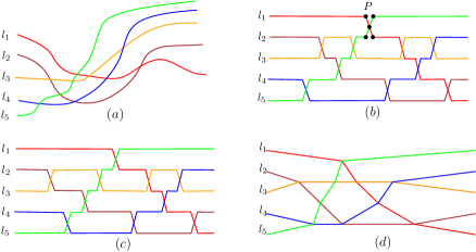
Figure 1: The reconstruction algorithm for PseodoLineArrangement.

Therefore, we can describe the LineArrangement problem as follows:

• Is it possible to stretch a PseudoLineArrangement of a given line arragement description such that each pseudo-line lies on a single line?

This problem is known as Stretchability. As stated before, pseudo-line arragement belongs to the $P$ complexity class and can be recognized and reconstructed efficiently(Algorithm 1). Therefore, $\exists\mathbb{R}\text{-}Completeness$ of LineArrangement implies that Stretchability is $\exists\mathbb{R}\text{-}Complete$.

Algorithm 1 Recognizing and Reconstruction algorithm for PseudoLineArrangement

2.3 Visibility graph of a polygon with holes

A polygon with holes is a simple polygon that has a set of non-colliding holes (simple polygons) inside it. The internal areas of the holes belong to the outside area of the polygon. In these polygons, two vertices are visible from each other if their connecting segment completely lies inside the polygon. Visibility graph of a polygon with holes is a graph whose vertices correspond to vertices of the polygon and holes, and in this graph there is an edge between two vertices if and only if their corresponding vertices in the polygon are visible from each other (see Fig. 2). In this paper, we assume that along with the visibility graph, we have the cycles that correspond to the order of vertices on the boundary of the polygon and the holes. The cycle that corresponds to the external boundary of the polygon is called the external cycle(see Fig. 2).

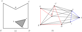
Figure 2: A polygon with one hole (a), and its visibility graph (b).

2.4 Internal-external visibility graphs

When we say that two points of a polygon are visible, it means that they see each other inside the polygon. However, the visibility can be defined similarly for the outside of the polygon. When we are going to talk about both of these visibilities, the former is called internal visibility and the latter is called external visibility. Precisely, two vertices are externally visible to each other if their connecting segment lies outside the polygon. Similarly, external visibility graph of a polygon is a graph whose vertices correspond to the vertices of the polygon, and its edges correspond to the external visibility relations. Having both these graphs separately is called the internal-external visibility graphs of a polygon(see Fig. 3).

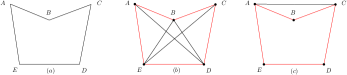
Figure 3: A polygon (a), its internal (b) and external (c) visibility graphs.

3 Complexity of Recognizing Visibility Graphs of Polygons with Holes

In this section, we show that recognizing visibility graph of a polygon with holes is $\exists\mathbb{R}\text{-}Complete$. This is done by reducing an instance of the stretchability problem to an instance of this problem.

In Section 2.2 we showed that we can describe the line arragement problem as an instance of stretchability of pseudo-lines in which each pseudo-line is composed of a chain of segments and the break-point vertices of these chains(except the first and the last endpoints of the chains) correspond to the intersection points of the pseudo-lines. We build a visibility graph $\mathcal{G}$, an external cycle $\mathcal{P}$, and a set of boundary cycles $\mathcal{H}$ from an instance of such a stretchability problem, and prove that the pseudo-line arragement is stretchable in the plane if and only if there exists a polygon with holes whose visibility graph is $\mathcal{G}$, its external cycle is $\mathcal{P}$ and the set of boundary cycles of its holes is $\mathcal{H}$.

Assume that $(\mathcal{L},\mathcal{S})$ is an instance of the stretchability problem where, as described in Algorithm 1, $\mathcal{L}=\langle l_{1},l_{2},...,l_{n}\rangle$ is the sequence of the pseudo-lines and $\mathcal{S}=\langle S_{1},S_{2},...,S_{n}\rangle$ is the sequence of the intersections of these pseudo-lines in which $S_{i}=\langle l_{a(i,1),...,a(i,n-1)}\rangle$ is the order of lines intersected by $l_{i}$. Let denote by $(\mathcal{G},\mathcal{P},\mathcal{H})$ the corresponding instance of the visibility graph realization in which $\mathcal{G}$ is the visibility graph, $\mathcal{P}$ is the external cycle of the outer boundary of the polygon and $\mathcal{H}=\{H_{1},H_{2},...,H_{k}\}$ is the set of boundary cycles of its holes. To build this instance, consider an example of such $(\mathcal{L},\mathcal{S})$ instance shown in Fig. 4-a. This figure shows a pseudo-line realization obtained from Algorithm 1 for an instance of four pseudo-lines. If this instance is stretchable, like the one shown in Fig. 4-b, we can build a polygon with holes like the one shown in Fig. 4-c. The outer boundary of this polygon and the boundary of its holes lie along a set of convex curves connecting the endpoints of each stretched pseudo-line. Precisely, for each stretched pseudo-line $l_{i}$, as in Fig. 4-b, there is a pair of convex chains in its both sides which connect its endpoints. This pair of pseudo-lines are sufficiently close to their corresponding stretched pseudo-lines, and their break-point vertices are the intersection points of these chains(like point $o$ in Fig. 4-c). This pair of convex chains, for each pseudo-line $l_{i}$, make a convex polygon which is called its channel and is denoted by $Ch(l_{i})$. The outer boundary of the target polygon and the boundary of its holes are obtained by removing those segments of the chains that lie inside another channel (see Fig. 4-c). Note that, we do not have the stretched realization of $(\mathcal{L},\mathcal{S})$ instance of the stretachability problem. But, from the pseudo-line realization, we can determine $\mathcal{G}$, $\mathcal{P}$ and $\mathcal{H}$ of the corresponding instance $(\mathcal{G},\mathcal{P},\mathcal{H})$ in polynomial time. As shown in Fig. 4-d, $\mathcal{P}$ and $\mathcal{H}$ are obtained by imaginary drawing a channel for each pseudo-line $l_{i}$. Finally, the vertex set of graph $\mathcal{G}$ is the set of all break-point vertices of these convex chains, and, two vertices are connected by an edge if and only if they belong to the boundary of the same channel. The following theorem shows the relationship between $(\mathcal{L},\mathcal{S})$ and $(\mathcal{G},\mathcal{P},\mathcal{H})$ problem instances.

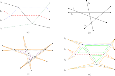
Figure 4: A polygon with holes which is constructed from an instance of the PseudoLineArrangement problem.

Theorem 3.1

An instance $(\mathcal{L},\mathcal{S})$ of the stretchability problem is realizable if and only if its corresponding $(\mathcal{G},\mathcal{P},\mathcal{H})$ instance of the visibility graph is recognizable.

Proof

When $(\mathcal{L},\mathcal{S})$ is stretchable, we can obtain a polygon with holes from the realization of $(\mathcal{L},\mathcal{S})$ whose external and holes boundaries are respectively correspond to $\mathcal{P}$ and $\mathcal{H}$. On the other hand, when the channels are sufficiently narrow and close to their line segments, each pair of vertices see each other if and only if they belong to the same channel. This means that their visibility graph is $\mathcal{G}$ and this polygon with holes is a realization for $(\mathcal{G},\mathcal{P},\mathcal{H})$ instance.

To prove the theorem in reverse, assume that the instance $(\mathcal{G},\mathcal{P},\mathcal{H})$ is realizable and we have a polygon $\mathcal{P}$ with holes $\mathcal{H}$ whose visibility graph is $\mathcal{G}$. In this realization, for the pair of endpoints of each channel consider the line that connects this pair of points. We claim that this set of lines is an answer for $(\mathcal{L},\mathcal{S})$ instance of the stretchability problem.

The induced subgraph of $\mathcal{G}$ on the vertices of a channel $C$ is a complete graph which implies that in the realization of $(\mathcal{G},\mathcal{P},\mathcal{H})$ these vertices must lie on the boundary of a convex polygon. On the other hand, each pair of channels $C_{i}$ and $C_{j}$ has exactly four vertices in common. Denote these common vertices by $Int(C_{i},C_{j})$. This set of common vertices forces that their corresponding lines (the lines that pass through the endpoints of these channels) must intersect in one point. Therefore, each pair of the obtained lines intersect in a point. To complete the proof, we must show that the intersections of these lines follow $\mathcal{S}$ and their initial vertical order is as $\mathcal{L}$. Consider the corresponding line $l$ of a channel $C$. The order of intersection points of $l$ and corresponding lines of other channels is directly derived from the order of common vertices between $C$ and other channels along the boundary of $C$. While these common vertices are either the vertices of $\mathcal{P}$ or cycles in $\mathcal{H}$, we can identify their order uniquely along the boundary of channel $C$. To do this, we first obtain the common vertices $Int(C,C_{i})$, which have two vertices on $\mathcal{P}$. This pair of vertices are connected to an endpoint of the channel $C$. This means that $l$ is first intersected by the corresponding line of $C_{i}$. Let $p,q$ be the other vertices in $Int(C,C_{i})$. These vertices either belong to $\mathcal{P}$ or a cycle in $\mathcal{H}$ and in both cases the next intersected channel is determined. When $p$ lies on $\mathcal{P}$, the next intersected channel is $C_{j}$ where $Int(C,C_{j})$ has a vertex adjacent to $p$ in $\mathcal{P}$, and, when $p$ lies on a cycle $H\in\mathcal{H}$, the next intersected channel is $C_{j}$ where $Int(C,C_{j})$ has a vertex adjacent to $p$ in $H$. Continuing this procedure, the order of intersection points of $l$ with other lines are uniquely determined which exactly is the same as $\mathcal{S}$. The reason is that we have built the channel and their common vertices according to $\mathcal{L}$. Finally, the initial order of these lines is the same as the order of endpoints of their corresponding channels along $\mathcal{P}$. Therefore, the initial vertical order of these lines will follow $\mathcal{L}$ by properly rotating the realization of the polygon for $(\mathcal{G},\mathcal{P},\mathcal{H})$.∎

It is easy to show that recognizing visibility graph of polygon with holes belong to $\exists\mathbb{R}$. While the stretchability problem is $\exists\mathbb{R}\text{-}Complete$ and our reduction is polynomial, Theorem 3.1 implies the $\exists\mathbb{R}\text{-}Hardness$ of recognizing visibility graph of polygon with holes. Therefore, we have the following theorem.

Theorem 3.2

Recognizing visibility graph of polygon with holes is $\exists\mathbb{R}\text{-}Complete$.

4 Complexity of Internal-External Visibility Graphs of a Simple Polygon

In this section, we show that recognizing internal-external visibility graph of a simple polygon is $\exists\mathbb{R}\text{-}Complete$. Again, we prove this by reducing an instance $(\mathcal{L},\mathcal{S})$ of the stretchability problem to an instance $(\mathcal{G}_{int},\mathcal{G}_{ext},\mathcal{P})$ of the visibility graph recognition where $\mathcal{G}_{int}$ and $\mathcal{G}_{ext}$ are respectively the internal and external visibility graphs and $\mathcal{P}$ is the external cycle of the boundary of the target simple polygon. Our construction of $(\mathcal{G}_{int},\mathcal{G}_{ext},\mathcal{P})$ is similar to the construction described in Section 3. We first build the same polygon with holes as in Section 3 with this difference that on each segment $ab$ on the boundary of a hole in $\mathcal{H}$, which $a$ and $b$ are intersection points of two convex chains, another point $c$ is added(Fig. 5-a) without violating the convexity of the channel chains. Then, we connect the holes together and to the external area to remove the holes and obtain a simple polygon. This is done iteratively on each hole by adding a pair of parallel and sufficiently close cut edges that connect a boundary segment of a hole to a segment of the current outer boundary. These cut edges. These segments must belong to different chains of the same channel and the pair of cut edges are close enough such that no pair $(p,q)$, in which $p$ and $q$ are not on the boundary of the same hole, be internally or externally visible to each other. These cut edges act as cutting channels like Fig. 5-b.

Trivially, the visibility graph of this simple polygon is no longer the same as the one obtained in Section 3. Having the stretched realization, we can compute internal and external visibility graphs of this simple polygon, which mainly depends on the way we cut the channels to remove the holes. In this polygon, two vertices are internally visible if and only if they belong to the same channel and their connecting segment does not cross any cut edge. In the external visibility graph, two vertices have an edge if and only if one of the following conditions hold:

• they are adjacent vertices on $\mathcal{P}$(points $a$ and $b$ in Fig. 5-b),

• they are endpoints of the edges of the same cut(points $c$ and $d$ in Fig. 5-b),

• they are vertices on different channel chains of the same hole (holes before cutting)(points $e$ and $f$ in Fig. 5-b),

• they lie on different channel chains and between two consecutive endpoints of the channels on $\mathcal{P}$(before cutting but including cut vertices)(points $g$ and $h$ or $g$ and $i$).

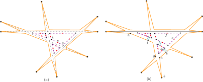
Figure 5: A simple polygon constructed from an instance of the PseudoLineArrangement problem.

Trivially, if $(\mathcal{L},\mathcal{S})$ is stretchable, its corresponding instance $(\mathcal{G}_{int},\mathcal{G}_{ext},\mathcal{P})$ is recognizable. To prove the reverse equivalence, we show in the next theorem that in any realization of $(\mathcal{G}_{int},\mathcal{G}_{ext},\mathcal{P})$ the boundary vertices of each channel must be a convex polygon. Then, by an argument similar to the one in Theorem 3.1, the stretchability of $(\mathcal{L},\mathcal{S})$ is equivalent to the realization of $(\mathcal{G}_{int},\mathcal{G}_{ext},\mathcal{P})$ as a simple polygon.

Theorem 4.1

In any realization of the internal-external visibility graph $(\mathcal{G}_{i}nt,\mathcal{G}_{e}xt,\mathcal{P})$, the lower and upper chains of each channel $C$ are convex.

Proof

For the sake of a contradiction, assume that there is a channel $C$ in the realization of $(\mathcal{G}_{int},\mathcal{G}_{ext},\mathcal{P})$ that is not a convex polygon. Except for the vertices of the cut edges, the pair of adjacent vertices to a vertex on $C$ are visible from each other in $\mathcal{G}_{int}$. Therefore, the internal visibility graph $\mathcal{G}_{int}$ forces that such a concavity on the boundary of $C$ must happen on some vertices of the cut edges that cross this channel. Without loss of generality, assume that such a concavity happens on the boundary of $C$ in Fig. 6, when we connect $O_{1}$ to $O_{2}$. The vertices $A_{1}$ and $O_{2}$ are non-visible pairs in $\mathcal{G}_{ext}$. According to Observation 2.1.2, they have at least one and at most two blocking vertices, one on the clockwise and the other on the counter-clockwise walks from $A_{1}$ to $O_{2}$. The vertex $O_{1}$ is such a blocking vertex on the counter-clockwise walk from $A_{1}$ to $O_{2}$. On the other hand, the last visible vertex from $A_{1}$ in $\mathcal{G}_{ext}$ along the clockwise walk on $\mathcal{P}$ toward $O_{2}$ is a vertex like $B_{2}$ and the last visible vertex from $O_{2}$ in $\mathcal{G}_{ext}$ along the counter-clockwise walk on $\mathcal{P}$ toward $A_{1}$ is another vertex like $B_{1}$ which is further than $B_{2}$ from $O_{2}$. Note that $O_{1}$ and $O_{2}$ lie on the boundary of the same hole before cutting and we have added extra vertices on all boundary segments of this hole. The vertices $A_{1}$, $B_{1}$ and $B_{2}$ are such extra and distinct vertices. Then, according to Observation 2, the non-visible pair $(A_{1},O_{2})$ does not have a blocking vertex in the clockwise walk from $A_{1}$ to $O_{2}$. Therefore, in any realization of $(\mathcal{G}_{int},\mathcal{G}_{ext},\mathcal{P})$, $O_{1}$ is the only blocking vertex of $A_{1}$ and $O_{2}$ which means that $O_{1}$ lies above the segment $A_{1}O_{2}$ and vertex $O_{1}$ is a convex vertex on the boundary of $C$. The same argument implies that $O_{2}$ is also a convex vertex on the boundary of $C$, which contradicts our assumption that $C$ is concave on $O_{1}$ or $O_{2}$.∎

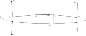
Figure 6: Upper and lower chains of a pseudo-line and their blocking vertices.

The above theorem implies that in any realization of $(\mathcal{G}_{int},\mathcal{G}_{ext},\mathcal{P})$, all channels are convex polygons. Therefore, by the same argument as Theorem 3.1, $(\mathcal{L},\mathcal{S})$ is stretchable if and only if $(\mathcal{G}_{int},\mathcal{G}_{ext},\mathcal{P})$ is recognizable. On the other hand, this reduction can be done in polynomial time and implies the $\exists\mathbb{R}\text{-}Hardness$ of recognizing internal-external visibility graphs of a simple polygon. It is easy to show that recognizing internal-external visibility graphs of a simple polygon belongs to $\exists\mathbb{R}$, and we obtain the following theorem.

Theorem 4.2

Recognizing internal-external visibility graphs of a simple polygon is $\exists\mathbb{R}\text{-}Complete$.

5 A Remark on BlockingVertexAssignment

In this section, we discuss the BlockingVertexAssignment and the question that whether having a BlockingVertexAssignment as a part of the input helps to solve the visibility graph recognition easier. Recall that, BlockingVertexAssignment of a visibility graph of a polygon is a function $\beta:V^{2}\rightarrow V$ that assigns a vertex to each non-visible ordered pair of vertices. This function introduced by Abello, et al., in 1994 matroid and indicates that which vertex has first blocked the visibility of an ordered pair of vertices. This blocking vertex is visible to the first vertex in the ordered non-visible pair and it is clear that every non-visible pair must have such a blocking vertex. There is another way to define a blocking vertex of an non-visible ordered pair: it is the first vertex in the shortest euclidean path inside the polygon from the first to the second vertex of an non-visible ordered pair. Such a path is unique inside a simple polygon, but, there can be more than one such paths between a pair of vertices of a polygon with holes. Moreover, two vertices on the boundary of a simple polygon can have two different shortest paths that lie outside the polygon. Therefore, BlockingVertexAssignment is not well-defined for visibility graph of a polygon with holes and for external visibility graph of a simple polygon. Abello et al., showed that a BlockingVertexAssignment must have four conditions, which are necessary conditions for a visibility graph to be recognizable. Later in 1997, Ghosh showed that these conditions are strictly stronger than Ghosh’s first three necessary conditions, but, strictly weaker than Ghosh’s four necessary conditions ghoshn . In 1995, Abello et al. introduced an algorithm that recognizes the visibility graph of 2-spiral polygons from its visibility graph and BlockingVertexAssignment in polynomial time twospiral . This result opened a question that whether having this function (BlockingVertexAssignment) as a part of the input makes computational complexity of recognizing visibility graphs of polygons easier? We show that recognizing internal-external visibility graphs is still $\exists\mathbb{R}\text{-}Complete$, when we have the BlockingVertexAssignment as a part of the input.

Theorem 5.1

BlockingVertexAssignment for the internal visibility graph of a polygon, constructed from PseudoLineArrangement problem, is unique and computable in polynomial time.

Proof

Consider a non-visible ordered pair $(a,b)$ and the blocking vertex function $\mathcal{B}$ for this polygon, where $a$ belongs to a channel $C$. Like any non-visible ordered pair, there are two candidates for $\mathcal{B}(a,b)$: last visible vertex in clockwise (name it $w$) and counter-clockwise (name it $c$) in a walk from $a$ toward $b$ on the external cycle. Both $c$ and $w$ are visible to $a$. Ghosh showed that these two candidates for blocking vertex see each other ghoshn . Therefore, $a$, $c$ and $w$ see each other and belong to the channel $C$.

On the other hand, $c$ and $w$ do not belong to the same common vertices of $Int(C,C_{j})$. For each pair of channels $(C_{i},C_{j})$, all vertices of $Int(C_{i},C_{j})$ are visible from previous and next vertices adjacent to the other three vertices in $Int(C_{i},C_{j})$. Therefore, by using Observation 2, if more than one of these three vertices belong to the clockwise (resp. counter-clockwise) walk from $a$ toward $b$, $(a,b)$ has no blocking vertex in clockwise (resp. counter-clockwise) walk from $a$ toward $b$.

Lets denote the three vertices which are in the same intersection set with $c$ by $o_{1}$, $o_{2}$ and $o_{3}$ and those which are in the same intersection set with $w$ by $o^{\prime}_{1}$, $o^{\prime}_{2}$ and $o^{\prime}_{3}$. If both $c$ and $w$ are blocking vertices, $o_{1}$, $o_{2}$ and $o_{3}$ belong to the clockwise walk from $a$ toward $b$ and in this walk we must meet them before $w$. Similarly, we must meet $o^{\prime}_{1}$, $o^{\prime}_{2}$ and $o^{\prime}_{3}$ before $c$ in the counter-clockwise walk from $a$ toward $b$. Hence, vertices $a$, $b$, $c$ and $w$ have an arrangement similar to the arrangement shown in Fig. 7. As shown in this figure, we cannot cross the convex area sorrounded by vertices of the channel $C$ which are visible from $a$ (like the area sorrounded by dotted orange, blue and green curves in Fig. 7). In all arrangements of these points, some of the adjacent vertices of at least one of these eight intersection points, will be trapped between the orange curve, the clockwise walk from $w$ toward $b$ and the counter-clockwise walk from $c$ toward $b$ (see $x$ and $y$ in Fig. 7). Therefore, we cannot meet these vertices before $w$ or $c$ in a clockwise or counter-clockwise walk from $a$ toward $b$ without crossing the convex area stated before. Consequently, we cannot have more than one visible blocking vertex from $a$ for the ordered non-visible pair $(a,b)$. Hence, the BlockingVertexAssignment for this kind of internal-external visibility graphs is unique.

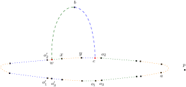
Figure 7: Determining BlockingVertexAssignment: Blue dotted lines correspond to some parts of the counter-clockwise walk from $a$ toward $c$ and the green dotted lines correspond to some parts of the clockwise walk from $a$ toward $w$. The blue dashed curve corresponds to the counter-clockwise curve from $c$ toward $b$ and the green dashed curve corresponds to the clockwise curve from $w$ toward $b$. Orange curve corresponds to the convex area which is visible from $a$.

On the other hand, we only use the first two Ghosh’s necessary conditions to find blocking vertices and these conditions can be verified in polynomial time ghoshn . So we can compute the BlockingVertexAssignment for this kind of polygons in polynomial time.∎

This theorem along with Theorem 4.2 imply that, if we have both internal and external visibility graphs of a simple polygon and its BlockingVertexAssignment as a part of input, the recognition problem is still $\exists\mathbb{R}\text{-}Complete$.

Theorem 5.2

Having the BlockingVertexAssignment for the internal visibility graph does not decrease the computational complexity class of recognizing internal-external visibility graphs of a simple polygon to a complexity class simpler class than $\exists\mathbb{R}\text{-}Complete$.

6 Conclusion

In this paper, we showed that the visibility graph recognition problem is $\exists\mathbb{R}\text{-}Complete$ for polygons with holes. Moreover, we showed that having both internal and external visibility graphs of a simple polygon, it is $\exists\mathbb{R}\text{-}Complete$ to recognize them as the visibility graphs of a simple polygon. Even, having the BlockingVertexAssignment of the internal visibility graph as a part of input, does not reduce the complexity class of this problem. This result motivates us to guess that having BlockingVertexAssignment for a visibility graph as a part of input does not decrease the computational complexity of realizing the visibility graphs of simple polygons. However, it is still open to determine the complexity class of the visibility graph recognition for a simple polygon. Although, having the external visibility graph and the BlockingVertexAssignment apply more constraints on reconstructing a simple polygon of a given visibility graph, but it may limit the possible choices of the realization. Therefore, our conjecture is that the visibility graph recognition problem for a simple polygon is still $\exists\mathbb{R}\text{-}Complete$.

References

- (1) Abello, J., Kumar, K.: Visibility graphs and oriented matroids. In: International Symposium on Graph Drawing, vol. LNCS 894, pp. 147–158. Springer (1994)
- (2) Abello, J., Kumar, K.: Visibility graphs of 2-spiral polygons. LATIN’95: Theoretical Informatics LNCS 911, 1–15 (1995)
- (3) Abello, J., Lin, H., Pisupati, S.: On visibility graphs of simple polygons. Congressus Numerantium pp. 119–119 (1992)
- (4) Abrahamsen, M., Adamaszek, A., Miltzow, T.: The art gallery problem is ∃ ℝ-complete. In: Proceedings of the 50th Annual ACM SIGACT Symposium on Theory of Computing, STOC 2018, pp. 65–73. ACM, New York, NY, USA (2018). DOI 10.1145/3188745.3188868. URL http://doi.acm.org/10.1145/3188745.3188868
- (5) Belta, C., Isler, V., Pappas, G.J.: Discrete abstractions for robot motion planning and control in polygonal environments. IEEE Transactions on Robotics 21(5), 864–874 (2005)
- (6) Bilò, V., Mavronicolas, M.: A Catalog of EXISTS-R-Complete Decision Problems About Nash Equilibria in Multi-Player Games. In: N. Ollinger, H. Vollmer (eds.) 33rd Symposium on Theoretical Aspects of Computer Science (STACS 2016), Leibniz International Proceedings in Informatics (LIPIcs), vol. 47, pp. 17:1–17:13. Schloss Dagstuhl–Leibniz-Zentrum fuer Informatik, Dagstuhl, Germany (2016). DOI 10.4230/LIPIcs.STACS.2016.17. URL http://drops.dagstuhl.de/opus/volltexte/2016/5718
- (7) Blum, L., Shub, M., Smale, S.: On a theory of computation and complexity over the real numbers: Np-completeness, recursive functions and universal machines. Bulletin of the American Mathematical Society 21(1), 1–46 (1989)
- (8) Boomari, H., Ostovari, M., Zarei, A.: Recognizing visibility graphs of polygons with holes and internal-external visibility graphs of polygons. arXiv preprint arXiv:1804.05105 (2018)
- (9) Boomari, H., Ostovari, M., Zarei, A.: Recognizing visibility graphs of triangulated irregular networks. Fundamenta Informaticae 179(4), 345–360 (2021)
- (10) Canny, J.: Some algebraic and geometric computations in pspace. In: Proceedings of the twentieth annual ACM symposium on Theory of computing, pp. 460–467. ACM (1988)
- (11) Cardinal, J.: Computational geometry column 62. SIGACT News 46(4), 69–78 (2015). DOI 10.1145/2852040.2852053. URL http://doi.acm.org/10.1145/2852040.2852053
- (12) Cardinal, J., Hoffmann, U.: Recognition and complexity of point visibility graphs. Discrete & Computational Geometry 57(1), 164–178 (2017)
- (13) Colley, P., Lubiw, A., Spinrad, J.: Visibility graphs of towers. Computational Geometry 7(3), 161–172 (1997)
- (14) Dobbins, M.G., Holmsen, A., Hubard, A.: Realization spaces of arrangements of convex bodies. Discrete & Computational Geometry 58(1), 1–29 (2017)
- (15) Everett, H.: Visibility graph recognition - phd thesis (1990)
- (16) Everett, H., Corneil, D.G.: Recognizing visibility graphs of spiral polygons. Journal of Algorithms 11(1), 1–26 (1990)
- (17) Garg, J., Mehta, R., Vazirani, V.V., Yazdanbod, S.: r-completeness for decision versions of multi-player (symmetric) nash equilibria. ACM Transactions on Economics and Computation (TEAC) 6(1), 1 (2018)
- (18) Ghosh, S.K.: On recognizing and characterizing visibility graphs of simple polygons. In: Scandinavian Workshop on Algorithm Theory, vol. LNCS 318, pp. 96–104. Springer (1988)
- (19) Ghosh, S.K.: On recognizing and characterizing visibility graphs of simple polygons. Discrete & Computational Geometry 17(2), 143–162 (1997)
- (20) Ghosh, S.K.: Visibility algorithms in the plane. Cambridge University Press (2007)
- (21) Goodman, J.E., Pollack, R.: Allowable sequences and order types in discrete and computational geometry. In: New trends in discrete and computational geometry, pp. 103–134. Springer (1993)
- (22) Herrmann, C., Ziegler, M.: Computational complexity of quantum satisfiability. J. ACM 63(2), 19:1–19:31 (2016). DOI 10.1145/2869073. URL http://doi.acm.org/10.1145/2869073
- (23) Hoffmann, U.: On the complexity of the planar slope number problem. J. Graph Algorithms Appl. 21(2), 183–193 (2017)
- (24) Hoffmann, U., Merckx, K.: A universality theorem for allowable sequences with applications. arXiv preprint arXiv:1801.05992 (2018)
- (25) Richter-Gebert, J.: Mnëv’s universality theorem revisited. Séminaire Lotaringien de Combinatorie (1995)
- (26) Schaefer, M.: Complexity of some geometric and topological problems. In: International Symposium on Graph Drawing, pp. 334–344. Springer (2009)
- (27) Shor, P.: Stretchability of pseudolines is np-hard. Applied Geometry and Discrete Mathematics-The Victor Klee Festschrift (1991)
- (28) Streinu, I.: Non-stretchable pseudo-visibility graphs. Computational Geometry 31(3), 195–206 (2005)
- (29) Teller, S., Hanrahan, P.: Global visibility algorithms for illumination computations. In: Proceedings of the 20th annual conference on Computer graphics and interactive techniques, pp. 239–246. ACM (1993)