Combining Enhanced Sampling with Experiment Directed Simulation of the GYG peptide

Abstract

Experiment directed simulation is a technique to minimally bias molecular dynamics simulations to match experimentally observed results. The method improves accuracy but does not address the sampling problem of molecular dynamics simulations of large systems. This work combines experiment directed simulation with both the parallel-tempering and parallel-tempering well-tempered ensemble replica-exchange methods to enhance sampling of experiment directed simulations. These methods are demonstrated on the GYG tripeptide in explicit water. The collective variables biased by experiment directed simulation are chemical shifts, where the set-points are determined by NMR experiments. The results show that it is possible to enhance sampling with either parallel-tempering and parallel-tempering well-tempered ensemble in the experiment directed simulation method. This combination of methods provides a novel approach for both accurately and exhaustively simulating biological systems.

1 Introduction

Molecular simulations are connected to experiments through ensemble properties, called observables. Often experimental and simulated values disagree, due to challenges such as limited accuracy of force-fields and discrepancies between how experiments can be represented in a simulation. This disagreement can be improved by adding an auxiliary biasing potential energy function^{1, 2}. For example, a simulation can be improved by incorporating experimental results as structural restraints in simulations³. Often these restraints are a type of harmonic energy penalty that brings conformational ensembles closer to the experimentally observed values ^{4, 5}. Visiting states that are outside structural restraints is unfavored with harmonic biases. This introduces some ambiguity in how strong these energetic restraints should be.

To address the ambiguity in using energetic restraints to match experimental data, a maximum entropy principle⁶ can be applied to find an energy bias that is minimal^{7, 8}. This bias acts only in the dimension of the collective variable which corresponds to the experimental observable⁹. Experiment directed simulation (EDS) is an implementation of maximum entropy biasing. EDS uses an adaptive biasing method to converge to the maximum entropy bias that achieves agreement between molecular simulation collective variables and experimental observables¹⁰. This bias is also provably the smallest change that can be made to match experimental data ^{8, 10, 11}.

EDS utilizes a single replica, whereas most other maximum entropy methods utilize multiple replicas¹. Other biasing methods, such as replica-exchange chemical shift restrained molecular dynamics simulations⁴ and restrained-ensemble molecular dynamics simulation method¹² that utilize multiple replicas require multiple replicas in order to match simulated results to some reference values. This increases the required computational effort, although there is an improvement in sampling due to the inherent increase of samples with the replicas. EDS, being a single-replica technique, provides no improvement to sampling. EDS has been applied to classical molecular dynamics¹⁰, ab-initio molecular dynamics¹³, and coarse-graining ¹⁴. EDS was able to give more accurate results on dynamic properties such as the self-diffusion coefficient of lithium in electrolyte solutions¹⁰, and the proton-diffusivity in ab initio water¹³ as well.

EDS is a biasing method and this is designed to match the ensemble average of some collective variable to a certain reference value. EDS lets the underlying simulation determine the fluctuations and underlying distribution of the collective variable. Only the expected value is shifted to match the experimental value. Because EDS is only a method of simulation, it cannot correct or mitigate any error in the reference value, such as experimental error, human error, or instrumentation error. If the experimental value is instead a distribution or becomes a distribution because a Bayesian inference approach with prior belief is desired, other techniques allow matching to that desired distribution like experiment directed metadynamics¹¹ or metainference¹⁵.

Aside from accuracy, another challenge in molecular dynamics simulations is sufficient sampling of phase space. The so-called “sampling problem”¹⁶ is especially true in solvated macromolecules, where systems can become trapped in energy minima. EDS introduces a bias in the potential to match experimental averages; it is not an enhanced sampling technique. Thus, there is a need to use an enhanced sampling techniques with EDS. Multiple enhanced sampling methods have been developed to alleviate this problem¹⁷, often by biasing sampling to occur along a certain collective variable¹⁸. This presents a complication with EDS if both an enhanced sampling technique and EDS are applied on the same set of collective variables. For example, metadynamics ¹⁹ will add Gaussian bias to the potential energy with respect to a collective variable, thereby modifying the potential of mean force (PMF) of that CV. EDS cannot be applied to a collective variable with a biased PMF, because EDS requires canonical samples. For example, if metadynamics is applied to $\Phi$ dihedral angle and EDS is applied $\Psi$ dihedral angle, the $\Psi$ angle needs to be re-weighted to achieve canonical sampling due to bias on $\Phi$ and the inherent correlation between the $\Phi$ and $\Psi$. EDS needs the $\Psi$ variable to be canonically sampled. Hence, EDS and Metadynamics cannot be applied simultaneously in a simulation. The well-tempered ensemble method (WTE) provides an alternative approach because it biases the fluctuations in energy, and with an assumption of the underlying potential energy distribution, does not affect the canonical sampling of other CVs. WTE can be further combined with parallel-tempering replica-exchange to improve sampling further^{20, 21, 22}.

In this work we consider the parallel-tempering well-tempered ensemble (PT-WTE) combined with EDS²² to improve both sampling and accuracy on an example system. Like in parallel-tempering replica-exchange, $N$ replicas of the simulation system are run concurrently. The coldest replica is the system of interest, yet it can escape free energy minima by swapping configurations with higher temperatures. The goal of PT-WTE is to reduce the number of replicas while maintaining similar replica efficiency²². It has been shown that PT-WTE metadynamics decreases the number of replicas from 100 to 10 while maintaining the similar energy landscape of solvated tryptophan-cage protein ²³. It has also been shown to improve speed of convergence to an accurate FES in model and real systems^{22, 23}. The technique can be applied to larger systems such as proteins to efficiently sample their large conformational space²⁴. The tri-peptide glycine-tyrosine-glycine (GYG) was used as a model system to demonstrate an implementation. GYG is found in structural and transport proteins such as collagen²⁵ and ion channels²⁶. Either mutations or complete deletions of this sequence from proteins showed either complete or partial loss of a function in those proteins ^{27, 28, 29}, so it has specific functional relevance. The experimental data utilized here is from backbone chemical shifts ³⁰ of GYG peptide. These are used to assess accuracy of the simulation and the free energy surface along the $\Phi$-$\Psi$ dihedral angles is used to assess sampling.

Metadynamics metainference³¹ and replica-averaged metadynamics³² are the nearest examples of the method proposed here in literature. Metadynamics metainferences is a combination of the enhanced sampling technique of metadynamics¹⁹ with the ability to match experimental data of metainference³¹. Replica-averaged metadynamics is the combination of the replica-averaging approach to matching experimental data³² with the enhanced sampling of metadynamics. A distinguishing difference between our approach and these is that the biasing force from EDS can be calculated with an enhanced-sampling method first and then be applied to a second simulation without replicas. This capability allows dynamic properties like autocorrelation functions or diffusivities to be computed.

2 Theory

In the WTE method²², Newton’s equation of motion becomes:

$$m\ddot{\mathbf{R}}=-\frac{U(\mathbf{R})}{\partial\mathbf{R}}-\frac{\partial V(U(\mathbf{R}),t)}{\partial\mathbf{R}}$$ (1)

where $m$ is the mass vector, $\mathbf{R}$ is the position vector, $U(\mathbf{R})$ is the system potential energy and $V(\cdot)$ is a time-dependent function of the instantaneous potential energy which biases the system. $V(\cdot)$ is defined with the following time-derivative:

$$\dot{V}(U,t)=\omega e^{-V(U,t)/k_{B}\Delta T}\delta{}(U-U(t))$$ (2)

where $\omega$ and $\Delta T$ are tuned constants. The intuition of this equation is to add a Guassian at each time $t$ centered at $U(t)$, just like in the metadynamics method ^{19, 33}. The key parameter in WTE is the bias factor, like in well-tempered metadynamics³³, which is defined relative to system temperature and $\Delta T$ as $\gamma=(T+\Delta T)/T$

Simulating according to this bias will asymptotically lead to the following distribution of potential energy, assuming normality of the potential energy probability distribution²²:

$$P(U)^{1/\gamma}\propto e^{\left(U-\left<U\right>\right)^{2}/2\gamma\Delta U^{2}}$$ (3)

where $\left<U\right>$ and $\Delta U^{2}$ are the expected value and variance of the potential energy of the unbiased canonical sampling. This expression shows that under the WTE bias, the average energies are the same but the variance of distribution is increased by $\sqrt{\gamma}$. A bias factor of 1 thus leads to canonical sampling. Increasing the bias factor increase the fluctuations in potential energy.

EDS modifies the potential energy of a system with a maximum entropy linear bias in a collective variable⁹. After equilibration, EDS will have the following biased potential energy:

$$U^{{}^{\prime}}(\mathbf{R})=U(\mathbf{R})+\alpha f(\mathbf{R})$$ (4)

where $\alpha$ is a Lagrange multiplier determined from an equilibration process described in White et al.¹⁰ and $f(\mathbf{R})$ is a differentiable collective variable. The $\alpha$ is selected such that $\left<f\right>=\hat{f}$, where $\hat{f}$ is a pre-determined value for what the expected value of the collective variable should be. In this work, we have experimentally determined NMR chemical shifts for $\hat{f}$. The limitation of EDS is that finding $\alpha$ requires calculating $\left<f\right>$ with good sampling of the underlying canonical distribution. The PT-WTE method can ensure we have sufficient sampling of the distribution of $f$ values. The WTE process only needs to be modified to replace $U(\mathbf{R})$ with $U^{{}^{\prime}}(\mathbf{R})$ and the previous analysis holds.

The benefit of WTE is that the increased energy fluctuations arising from the choice of bias factor can improve replica-exchange efficiency in a parallel-tempering setting. The probability of exchange for replicas $i$ and $j$ becomes³⁴:

$$P(\textrm{ex}\,i,j)=\textrm{min}\left[1,\exp\left(\gamma^{-1}\beta_{i}\left[U_{i}^{{}^{\prime}}(\mathbf{R}_{i})-U_{i}^{{}^{\prime}}(\mathbf{R}_{j})\right]+\gamma^{-1}\beta_{j}\left[U_{j}^{{}^{\prime}}(\mathbf{R}_{j})-U_{j}^{{}^{\prime}}(\mathbf{R}_{i})\right]\right)\right]$$ (5)

where $\beta_{i}=1/k_{B}T_{i}$ and $U_{i}^{{}^{\prime}}$ is the potential energy of the $i$th replica including the EDS bias. Note that EDS will have different $\alpha$ for each replica because $\left<f\right>$ is a function of temperature. This exchange rule ensures that the resulting simulation will arrive at a canonical distribution without re-weighting. The result of this method is both an enhanced-sampled ensemble and a value for $\alpha$.

3 Methods

A short peptide GYG was simulated with EDS¹⁰ and PT-WTE²² to enhance sampling and improve fit to experimental NMR chemical shifts from Platzer et al.³⁰. To compare the performance of EDS with enhanced sampling to other simulations, EDS with PT-WTE was compared to a single replica unbiased simulation, a single replica biased simulation, a parallel-tempering replica-exchange molecular dynamics (PT) simulation, and replica unbiased PT-WTE simulation.

0.008 mg/cm³ GYG peptide in 10 mM NaCl counter-ions was first energy minimized then annealed and equilibrated in the NVT ensemble using the Canonical Sampling through Velocity Rescaling (CSVR) thermostat³⁵. The CHARM27³⁶ force field and TIP3P³⁷ water model were used throughout. Electrostatic forces were calculated with the particle mesh Ewald method ³⁸, and dispersion forces were calculated with shifted Van der Waals potentials with a cutoff distance of 10 Å. The covalent hydrogen bonds were constrained using the LINCS algorithm ³⁹ to enable a 2 fs time step. All simulations were performed in the Gromacs-5.1.4 simulation engine⁴⁰. To automatically run Gromacs commands in python, GromacsWrapper was used⁴¹. To generate an initial extended structure of GYG, the python package PeptideBuilder was used⁴².

An equilibration is required for the PT-WTE method. 16 replicas of PT-WTE were tuned for 400 ps to find parameters that gave increased replica efficiency. The replica temperatures used for the 16 replica systems were 293, 299, 304, 310, 316, 323, 329, 336, 342, 349, 355, 363, 370, 377, 385, 392 K, as generated by the method of Nemoto et al. ⁴³. The exchanges were attempted every 250 time steps. The WTE parameters were chosen following Barducci et al. ³³ and are shown in Table 1.

After the aforementioned short PT-WTE equilibration step, EDS was begun with the static bias from PT-WTE equilibration step. This combined PT-WTE with EDS had 16 replicas with the same set of temperatures as mentioned above and was 40 ns long. To control against the presence of either EDS bias, or PT-WTE bias, or both biases, 16 replica 40 ns PT simulations with and without EDS bias in the absence of WTE bias and 16 replica 40 ns PT-WTE simulations with and without EDS bias were run and as shown in Table 1. The large amount of time is not necessary for convergence of EDS, but was chosen to get good sampling statistics. The EDS collective variables biased were chemical shifts³⁰ calculated via the Plumed2 molecular simulation plugin⁴⁴. The EDS parameters chosen are shown in Table 1.

An 8 replica PT-WTE simulation was also done with and without EDS. These simulations demonstrate how PT-WTE can use fewer replicas than PT and still achieve good efficiency. The parameters are in Table 1. The replicas ran at the following temperatures: 293, 306, 320, 335, 350, 366, 383, and 400 K. Similar to 16 replica PT-WTE, 8 replica PT-WTE initially consisted of 400 ps equilibration step, followed by a static production step of 40 ns. There were 3620 atoms in the simulation with 1197 tip3p water molecules and 38 peptide atoms. We used bias factor of 10 for 16 replica PT-WTE and 20 for 8 replica PT-WTE. Deighen et al. studied the effect of bias factor in 10 replica simulation that studied 39 amino acids long Trp-cage protein ²³. They found that increasing the bias factor from 10 to 24 decreased the the time it takes to converge to the reference FES²³. Hence, we used larger bias factor for 16 replica PT-WTE compared to 8 replica PT-WTE.

Overview of simulation systems and their parameters.
Simulation	EDS+	No EDS+	EDS+	No EDS+	Exp(b)
Parameters	PT-WTE(a)	PT-WTE(a)	PT	PT
Replicas	16	16	16	16	-
Bias factor	10	10	-	-	-
Hill width$\left(\frac{\textrm{kJ}}{\textrm{mol}}\right)$	100	100	-	-	-
Hill height $\left(\frac{\textrm{kJ}}{\textrm{mol}}\right)$	0.1	0.1	-	-	-
Dim. Prop	0.2	-	0.2	-	-
Range	0.01	-	0.01	-	-
Time (ns)	40(0.4(a))	40(0.4(a))	40	40	-
Results
C$\beta$ $\delta$ (ppm)	38.52$\pm$2.35	36.39$\pm$2.13	38.48$\pm$1.84	39.06$\pm$2.89	38.60$\pm$0.08
C$\alpha$ $\delta$ (ppm)	57.89$\pm$3.21	59.38$\pm$ 2.35	57.93$\pm$3.25	58.23$\pm$3.34	58.00$\pm$0.08
H $\delta$ (ppm)	8.29$\pm$0.50	8.20$\pm$0.48	8.20$\pm$0.46	8.25$\pm$0.47	8.16$\pm$0.02
H$\alpha$ $\delta$ (ppm)	4.58$\pm$0.51	4.04$\pm$0.52	4.54$\pm$0.42	4.61$\pm$0.55	4.55$\pm$0.02
CO $\delta$ (ppm)	176.28$\pm$1.30	174.78$\pm$1.11	176.25$\pm$1.26	175.34$\pm$1.64	176.30$\pm$0.08
N $\delta$ (ppm)	120.06$\pm$5.34	118.34$\pm$7.43	120.09$\pm$5.35	119.88$\pm$6.58	120.1$\pm$0.08
Repl Efficiency (%)	39(31(a))	21(31(a))	22	23	-
Aver Efficiency (%)	41(40(a))	28.2(40(a))	23	25	-

Overview of simulation systems and their parameters.
Simulation	EDS+	No EDS+	EDS+	No EDS+	Expb
Parameters	PT-WTE	PT-WTE	No PT	No PT
Replicas	8	8	1	1	-
Bias factor	20	20	-	-	-
Hill width$\left(\frac{\textrm{kJ}}{\textrm{mol}}\right)$	250	250	-	-	-
Hill height $\left(\frac{\textrm{kJ}}{\textrm{mol}}\right)$	1	1	-	-	-
Dim. Prop	0.2	-	0.2	-	-
Range	0.001	-	0.01	-	-
Time (ns)	40(0.4(a))	40(0.4(a))	40	40	-
Results
C$\beta$ $\delta$ (ppm)	38.48$\pm$2.06	37.77$\pm$3.05	38.47$\pm$1.71	39.18$\pm$2.58	38.60$\pm$0.08
C$\alpha$ $\delta$ (ppm)	57.94$\pm$3.35	58.91$\pm$3.14	57.94$\pm$3.06	57.99$\pm$3.33	58.00$\pm$0.08
H $\delta$ (ppm)	8.20$\pm$0.47	8.22$\pm$0.48	8.37$\pm$0.50	8.21$\pm$0.49	8.16$\pm$0.02
H$\alpha$ $\delta$ (ppm)	4.54$\pm$0.45	4.26$\pm$0.61	4.54$\pm$0.41	4.68$\pm$0.51	4.55$\pm$0.02
CO $\delta$ (ppm)	176.25$\pm$1.30	175.00$\pm$1.55	176.30$\pm$1.14	175.40$\pm$1.54	176.30$\pm$0.08
N $\delta$ (ppm)	120.12$\pm$5.49	117.90$\pm$7.20	120.01$\pm$4.79	119.43$\pm$5.84	120.1$\pm$0.08
Repl Efficiency (%)	55 (40(a))	43(39(a))	-	-	-
Aver Efficiency (%)	62 (51(a))	58(53(a))	-	-	-

Table 1. These are the computed averages during various simulations. 2.5^th and 97.5^th percentile of the computed values are shown as well. The EDS and PT-WTE parameters are shown first as well as the simulation time. The chemical shifts are the cumulative averages. The replica-exchange efficiency is the percentage of attempted replica swaps that are successful for the least efficient replica. The average is the efficiency averaged over all replicas.

a-PT-WTE was equilibrated for 400 ps and then restarted without further addition of gaussian hills for the 40 ns simulation. RMSD due to Camshift⁴⁵ for N,HN,HA,CA,CB, and C are 3.01,0.56,0.28,1.3,1.36 and 1.38 ppm.

b-Experimental values are from Platzer et al ³⁰

4 Results & Discussion

Table 1 provides an overview of the simulations run for this work. Multiple combinations of enhanced sampling methods with and without EDS were simulated. Each simulation ran for 40 ns. The 16 replica PT-WTE simulations were equilibrated for 400 ps to find the biasing potentials that increased the replica-exchange efficiency, prior to enabling EDS. This PT-WTE tune step was run long enough to ensure the efficiency exceeded 30%. Parallel-tempering replica-exchange (PT) with 16 replicas has 23% replica efficiency, as shown in Table 1. The replica efficiency is defined here as the minimum acceptance rate of configuration swapping between replicas. In other words, the lowest among the 16 replicas is taken to be the efficiency. This ensures that all replicas exchange at certain threshold rate prohibiting a different independent system of simulations that are exchanging only with replicas that have closer temperatures. The averages are also shown for the 40ns simulations. Replica-exchange of 20% is the minimum for a well-sampled system⁴⁰, and thus 16 was the minimum number of replicas for PT.

The choice of PT-WTE simulation parameters achieved good exchange with the smaller, 8 replica system, despite spanning the same temperature range as the 16 replica systems (293K to 400K). Since 8 replica system had a different set of WTE parameters, EDS parameters were modified as well, which included the reduction of the speed of convergence of EDS (lower range parameter) and the increase the speed of convergence of the PT-WTE method (larger hill height)²². The bias factor was correspondingly decreased to reduce the strength of bias more quickly. PT-WTE with 16 replicas had smaller replica efficiency than 8 replica PT-WTE in Table 1. This may be the result of a different set WTE and EDS parameters used in 8 replica and 16 replica simulations.

The EDS method moved the calculated backbone chemical shifts to the experimental values when applied as seen in Table 1. There is good agreement between the average chemical shifts in the EDS simulations and experiments with any of the enhanced sampling methods applied. Even with the slower parameters used in the 8 replica system, the EDS method still achieved the correct values.

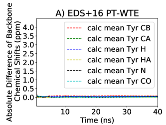
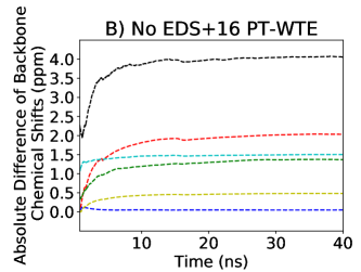
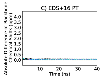
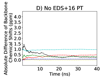
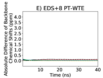
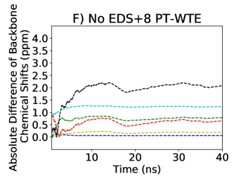
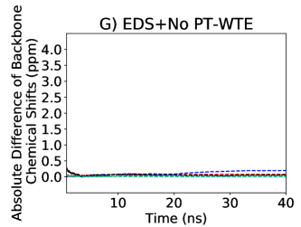
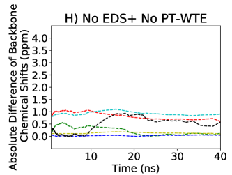
Figure 1: Convergence of chemical shifts to the reference experimental value. Absolute difference between calculated and experimental chemical shifts. EDS was used with PT-WTE for enhanced sampling as shown in (a). (b) shows that without EDS. (c) EDS with 16 replica PT converges to experiments. The lack of EDS lowers the convergence (d). (e) displays with fewer replicas, EDS still converges to experiments.(f) Without EDS, convergence is lower.

Figure 1 shows the cumulative calculated mean backbone chemical shifts over time during 16 replica PT-WTE with EDS bias (a), 16 replica PT-WTE without EDS (b), 16 replica PT with EDS (c), 16 replica PT without EDS, 8 replica PT-WTE with EDS (e), 8 replica PT-WTE without EDS (f), single replica EDS (g), and a standard MD (h). Chemical shifts were modified to show the absolute difference between cumulative averages and the corresponding experimental chemical shifts. Therefore, exact match between simulation and experiment is indicated by the convergence of cumulative calculated mean chemical shifts to 0. As expected, EDS biased average chemical shifts converge to the reference value with 16 replica PT-WTE (Fig. 1a), with 16 replica PT (Fig. 1c), and with 8 replica PT-WTE (Fig. 1e). EDS does not make instantaneous values of biased chemical shifts converge with the reference value, but makes the ensemble average to approach the reference value as shown in fig. S1 of the Supporting Information. In all of the EDS cases (fig. 1a, 1c, 1e, and 1g), EDS converges within 1 ns. In all EDS bias simulations (fig. 1a, 1c, 1e, and 1g), average chemical shifts of the hydrogen connected to backbone nitrogen atom had the highest deviation from predicted value compared to other atoms. The Camshift root mean square deviation for H connected to N is 0.56 ppm, whereas Camshift predicts deviations to be highest for N with RMSD of 3.01 ppm in a 28 protein test set⁴⁵. During 40 ns simulation, the cumulative average backbone HN chemical shift was within 1 % of the reference chemical shift. Since PT-WTE and PT swaps configurations between different temperature replicas, chemical shifts also change whenever the conformations change as indicated by the greater fluctuations between mean chemical shifts and reference values in PT-WTE and PT with EDS (Fig. 1a, 1c, and 1d ) simulation compared to single replica EDS (Fig. 1g). In the absence of EDS bias, average chemical shifts in various simulations, shown in figures 1b, 1d, 1e, and 1f, do not converge to 1 because the simulation is less accurate. When EDS was absent in both 16 replica PT-WTE (Fig. 1b) and 16 replica PT (Fig. 1d), average chemical shifts fluctuated more drastically in Fig. 1b compared to simulation without PT-WTE as shown in Fig. 1d. This is due to the better exploration of phase-space with the PT-WTE method. The convergence under a variety of enhanced sampling methods shows that EDS still works well when combined with enhanced sampling.

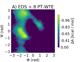
(a)

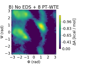
(b)

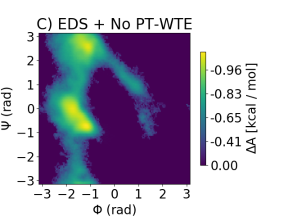
(c)

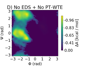
(d)

Figure 2: Free Energy Surface (FES) of $\Phi$-$\Psi$ dihedral angles of Y amino acid from GYG simulations. (a) shows the FES with EDS and PT-WTE so that backbone chemical shifts match experimental values and sampling is enhanced. (b) without EDS bias, PT-WTE explores $\Phi$ around 1.5 and $\Psi$ in -3.14,3.14 radians interval more, and finds a global minimum at about $\Phi$=1.5,$\Psi$=1 rad. (c) shows less sampling of global minimum at $\Phi$=1.5 radians and $\Psi$=1 radians,compared to a). (d) shows no exploration of the global minimum at $\Phi$=1.5 and $\Psi$=1 rad and seems to be stuck on negative $\Phi$ angles. All FESs were generated from a 20 ns NVT simulation at 293K

To see the effect of enhanced sampling and the effect of biased chemical shifts to other collective variables in a simulation, $\Phi$ and $\Psi$ dihedral angles were compared to regular unbiased MD and to Ramachandran plots from X-ray crystallography⁴⁶. The simulated free energy landscapes of Tyrosine in GYG peptide along $\Phi$ and $\Psi$ dihedral angles are displayed in Fig. 2. Dihedral angles were computed during the simulations and their histograms were used to compute the FES. EDS predicted the same global minimum regardless of presence (Fig.  2a) or absence of PT-WTE (Fig.  2c) at $\Phi$=-1.2 and $\Psi$=-0.9. The free energy surface shows different global minimum with EDS because the free energy distribution is biased to satisfy experimental conditions. As shown in figures  2a and  2c, EDS simulations show the global minimum to be at $\Phi$=-1.2 and $\Psi$=-0.9 radians, different from the one observed by enhanced sampling alone (Fig.  2b). Enhanced sampling technique found a different global minimum at $\Phi$=1 and $\Psi$=1, in the absence of EDS than in the presence of EDS. Also, PT-WTE without EDS enabled the exploration of a region at $\Phi$=1 and $\Psi$ in interval [-3.14,3.14] radians in figure  2b which is similar to Tyrosine Ramachandran map from Vitalini et al⁴⁷; neither of EDS alone (Fig. 2c), EDS with PT-WTE (Fig. 2a) and regular MD (Fig. 2d) could sample around that region continuously. Although EDS in the presence of PT-WTE (Fig. 2a), did not show aberrant behavior from absence of PT-WTE in figure  2c, it showed improved sampling of global minimum observed in PT-WTE alone at $\Phi$ around 1 radians and at $\Psi$=1 radians compared to the absence of PT-WTE (Fig. 2c) and regular MD (Fig.  2d). Overall, PT-WTE improved sampling and EDS modified the FES to achieve agreement with the NMR chemical shifts.

Ramachandran plots from Ting et al.⁴⁶ of Tyrosine in the sequence GYG were compared to our results. The Ting et al.⁴⁶ results are derived from a bioinformatics analysis of X-ray crystallographic data of whole proteins. Tyrosine dihedral angle plot of Tyrosine in YG peptide from Ting et al.⁴⁶, was compared to our results, since YG was closest GYG. Ting et al, observed three regions of minimum in Tyrosine: at about ($\Phi$=-1.0,$\Psi$=2.8, which was the global minimum), ($\Phi$=-1.0,$\Psi$=[-1,1] interval), and ($\Phi$=1,$\Psi$=1) rad. Out of all the FES for simulations that are shown, Fig. 2a was closest to experimentally observed FES by Ting et al.⁴⁶, because, local minimum at ($\Phi$=1,$\Psi$=1) was predicted correctly and minima at ($\Phi$=-1.0,$\Psi$=2.8) and ($\Phi$=-1.0,$\Psi$=[-1,1] interval) were close relative to each other in Ting et al.⁴⁶ and in Fig. 2a. Ting et al.⁴⁶ also reported the global minima to be on the negative $\Phi$ angle axis. Without EDS, enhanced sampling alone could not label the experimentally observed global minimum as global minimum at $\Phi$=-1 and $\Psi$=2.8 in Fig. 2b. $\Psi$ global minimum was around zero for both Ting et al.⁴⁶ and EDS results (Fig. 2a and  2c). A local minimum at around $\Phi$=1 and $\Psi$=1 radians reported by Ting et al.⁴⁶, was also observed as a minimum Fig. 2a,  2b, and  2c. This local minimum was not predicted by standard MD at all within 20 ns, as seen in Fig. 2d. EDS did not show drastic deviation in unbiased structural properties, such as a dihedral angle of Tyrosine. Indeed dihedral angles in EDS simulations with or without enhanced sampling showed similar results as X-ray crystallography did.

Another major question about disagreement between simulations and experiments is whether the underlying cause is lack of sampling or inaccuracy of the force-field/system. The 8 replica PT-WTE without EDS shows that even with good sampling, the simulation matches neither the chemical shifts nor the FES from the EDS simulation, as shown in Fig. 2b. This is not necessarily due to a deficiency in the CHARMM force field, but instead could be due to a difference in concentration, ions, and termini between the simulations and the work of Platzer et al. ³⁰, from which the chemical shifts were measured.

5 Conclusion

Simultaneous enhanced sampling and experiment directed simulation (EDS) was demonstrated on the GYG peptide in explicit solvent. EDS improved the accuracy of the simulation by minimally biasing the backbone chemical shifts of the peptide to match experimental data from Platzer et al³⁰. Single replica simulations with and without EDS bias ran for comparable time. Both parallel-tempering replica-exchange (PT) and parallel-tempering well-tempered ensemble (PT-WTE) were used with EDS to improve sampling. Compared to absence of enhanced sampling in a control MD, system has significantly benefited from enhanced sampling. PT and PT-WTE provided improved sampling and did not interfere with EDS, with EDS converging within 1 ns. On the same computer architecture, 16 replica PT-WTE simulations and 16 replica PT with and without EDS completed after approximately the same period of wall-clock time. PT-WTE with 8 replicas spanning 293K to 400K was also demonstrated with EDS, showing that the PT-WTE method is able to reduce the number of replicas required relative to PT while not jeopardizing enhanced sampling. We have demonstrated that PT-WTE and PT can be applied with EDS simultaneously without interfering with each other in this system. We will exploit this new method on larger system of proteins and peptides, to take advantage of both enhanced sampling as well as biasing with experiments.

6 Acknowledgements

Support for DB Amirkulova provided by a Hopeman scholarship from University of Rochester. Thanks to Rainier Barret for feedback and discussion of manuscript. We are grateful for resources and services provided by Center for Integrated Research Computing at University of Rochester.

References

- 1 M. Bonomi, G. T. Heller, C. Camilloni, and M. Vendruscolo, “Principles of protein structural ensemble determination,” Current Opinion in Structural Biology, vol. 42, pp. 106–116, 2017.
- 2 J. R. Allison, “Using simulation to interpret experimental data in terms of protein conformational ensembles,” Current Opinion in Structural Biology, vol. 43, pp. 79–87, 2017.
- 3 A. Cavalli, X. Salvatella, C. M. Dobson, and M. Vendruscolo, “Protein structure determination from NMR chemical shifts,” Proc Natl Acad Sci U S A, vol. 104, no. 23, pp. 9615–9620, 2007.
- 4 P. Robustelli, K. Kohlhoff, A. Cavalli, and M. Vendruscolo, “Using NMR chemical shifts as structural restraints in molecular dynamics simulations of proteins,” Structure, vol. 18, no. 8, pp. 923–933, 2010.
- 5 A. E. Torda, R. M. Scheek, and W. F. van Gunsteren, “Time-averaged Nuclear Overhauser Effect Distance Restraints Applied to Tendimistat,” J.Mol.Biol., vol. 214, pp. 223–235, 1990.
- 6 E. Jaynes, “Information Theory and Statistical Mechanics,” Physical Review A, vol. 106, no. 4, pp. 620–621, 1957.
- 7 W. Boomsma, J. Ferkinghoff-borg, and K. Lindorff-larsen, “Combining Experiments and Simulations Using the Maximum Entropy Principle,” PLOS Comput. Biol., vol. 10, no. 2, pp. 1–9, 2014.
- 8 B. Roux and J. Weare, “On the statistical equivalence of restrained-ensemble simulations with the maximum entropy method,” Journal of Chemical Physics, vol. 138, no. 8, 2013.
- 9 J. W. Pitera and J. D. Chodera, “On the use of experimental observations to bias simulated ensembles,” Journal of Chemical Theory and Computation, vol. 8, no. 10, pp. 3445–3451, 2012.
- 10 A. D. White and G. A. Voth, “Efficient and Minimal Method to Bias Molecular Simulations with Experimental Data,” Journal of Chemical Theory and Computation, vol. 10, no. 8, pp. 3023–3030, 2014.
- 11 A. D. White, J. F. Dama, and G. A. Voth, “Designing Free Energy Surfaces That Match Experimental Data with Metadynamics,” Journal of Chemical Theory and Computation, vol. 11, no. 6, pp. 2451–2460, 2015.
- 12 S. Roux, Benoit and Islam, “Restrained-Ensemble Molecular Dynamics Simulations Based on Distance Histograms from Double Electron-Electron Resonance Spectroscopy,” J Phys Chem B, vol. 17, no. 117, pp. 4733–4739, 2013.
- 13 A. D. White, C. Knight, G. M. Hocky, and G. A. Voth, “Communication: Improved ab initio molecular dynamics by minimally biasing with experimental data,” Journal of Chemical Physics, vol. 146, no. 4, 2017.
- 14 T. Dannenhoffer-Lafage, A. D. White, and G. A. Voth, “A Direct Method for Incorporating Experimental Data into Multiscale Coarse-grained Models.,” Journal of chemical theory and computation, vol. 12, no. 5, pp. 2144–2153, 2016.
- 15 M. Bonomi, C. Camilloni, A. Cavalli, and M. Vendruscolo, “Metainference: A Bayesian inference method for heterogeneous systems,” Science advances, vol. 2, no. 1, p. e1501177, 2016.
- 16 J. B. Clarage, T. Romo, B. K. Andrews, B. M. Pettitt, and G. N. Phillips, “A sampling problem in molecular dynamics simulations of macromolecules.,” Proceedings of the National Academy of Sciences of the United States of America, vol. 92, no. 8, pp. 3288–3292, 1995.
- 17 R. C. Bernardi, M. C. Melo, and K. Schulten, “Enhanced sampling techniques in molecular dynamics simulations of biological systems,” Biochimica et Biophysica Acta (BBA) - General Subjects, vol. 1850, no. 5, pp. 872–877, 2015.
- 18 E. Darve, D. Rodriguez-Gomez, and A. Pohorille, “Adaptive biasing force method for scalar and vector free energy calculations,” Journal of Chemical Physics, vol. 128, no. 14, pp. 1–13, 2008.
- 19 A. Laio and M. Parrinello, “Escaping free-energy minima.,” Proceedings of the National Academy of Sciences of the United States of America, vol. 99, no. 20, pp. 12562–12566, 2002.
- 20 U. H. E. Hansmann, “Parallel tempering algorithm for conformational studies of biological molecules,” Chemical Physics Letters, vol. 281, no. or L, pp. 140–150, 1997.
- 21 E. Bittner, A. Nubaumer, and W. Janke, “Make life simple: Unleash the full power of the parallel tempering algorithm,” Physical Review Letters, vol. 101, no. 13, pp. 1–4, 2008.
- 22 M. Bonomi and M. Parrinello, “Enhanced sampling in the well-tempered ensemble,” Physical Review Letters, vol. 104, no. 19, pp. 1–4, 2010.
- 23 M. Deighan, M. Bonomi, and J. Pfaendtner, “Efficient simulation of explicitly solvated proteins in the well-tempered ensemble,” Journal of Chemical Theory and Computation, vol. 8, no. 7, pp. 2189–2192, 2012.
- 24 V. Spiwok, Z. Sucur, and P. Hosek, “Enhanced sampling techniques in biomolecular simulations,” Biotechnology Advances, vol. 33, no. 6, pp. 1130–1140, 2015.
- 25 J. Bella, J. Liu, R. Kramer, B. Brodsky, and H. M. Berman, “Conformational Effects of Gly – X – Gly Interruptions in the Collagen Triple Helix,” J. Mol. Biol., vol. 362, pp. 298–311, 2006.
- 26 K. M. Dibb, T. Rose, S. Y. Makary, T. W. Claydon, D. Enkvetchakul, R. Leach, C. G. Nichols, and M. R. Boyett, “Molecular Basis of Ion Selectivity , Block , and Rectification of the Inward Rectifier Kir3 . 1 / Kir3 . 4 K ؉ Channel,” Journal of Biological Chemistry, vol. 278, no. 49, pp. 49537–49548, 2003.
- 27 G. Thiagarajan, Y. Li, A. Mohs, C. Strafaci, M. Popiel, J. Baum, and B. Brodsky, “Common Interruptions in the Repeating Tripeptide Sequence of Non-fibrillar Collagens : Sequence Analysis and Structural Studies on Triple-helix Peptide Models,” J. Mol. Biol, pp. 736–748, 2008.
- 28 I. So, I. Ashmole, N. W. Davies, M. J. Sutcliffe, and P. R. Stanfield, “The K + channel signature sequence of murine Kir2 . 1 : mutations that affect microscopic gating but not ionic selectivity,” Journal of Physiology, vol. 531, no. 1, pp. 37–50, 2001.
- 29 S. Bernèche and B. Roux, “A Gate in the Selectivity Filter of Potassium Channels,” Structure, vol. 13, pp. 591–600, 2005.
- 30 G. Platzer, M. Okon, and L. P. Mcintosh, “pH-dependent random coil 1 H , 13 C , and 15 N chemical shifts of the ionizable amino acids : a guide for protein p K a measurements,” Journal of Biomolecular NMR, pp. 109–129, 2014.
- 31 M. Bonomi, C. Camilloni, and M. Vendruscolo, “Metadynamic metainference: Enhanced sampling of the metainference ensemble using metadynamics,” Scientific Reports, vol. 6, no. July, pp. 1–11, 2016.
- 32 C. Camilloni, A. Cavalli, and M. Vendruscolo, “Replica-averaged metadynamics,” Journal of Chemical Theory and Computation, vol. 9, no. 12, pp. 5610–5617, 2013.
- 33 A. Barducci, G. Bussi, and M. Parrinello, “Well-tempered metadynamics: A smoothly converging and tunable free-energy method,” Physical Review Letters, vol. 100, no. 2, pp. 1–4, 2008.
- 34 G. Bussi, “Hamiltonian replica exchange in GROMACS: A flexible implementation,” Molecular Physics, vol. 112, no. 3-4, pp. 379–384, 2014.
- 35 G. Bussi, D. Donadio, and M. Parrinello, “Canonical sampling through velocity rescaling,” Journal of Chemical Physics, vol. 126, no. 1, 2007.
- 36 R. W. Pastor and A. D. MacKerell Jr., “Development of the CHARMM Force Field for Lipids.,” Journal of Physical Chemistry Letters, vol. 2, no. 13, pp. 1526–1532, 2011.
- 37 W. L. Jorgensen, J. Chandrasekhar, J. D. Madura, R. W. Impey, and M. L. Klein, “Comparison of simple potential functions for simulating liquid water,” The Journal of Chemical Physics, vol. 79, no. 2, pp. 926–935, 1983.
- 38 U. Essmann, L. Perera, M. L. Berkowitz, T. Darden, H. Lee, and L. G. Pedersen, “A smooth particle mesh Ewald method A smooth particle mesh Ewald method,” The Journal of Chemical Physics, vol. 103, no. 19, pp. 8577–8593, 1995.
- 39 B. Hess, H. Bekker, H. J. C. Berendsen, and J. G. E. M. Fraaije, “LINCS: A linear constraint solver for molecular simulations,” Journal of Computational Chemistry, vol. 18, no. 12, pp. 1463–1472, 1997.
- 40 M. James, T. Murtola, R. Schulz, J. C. Smith, B. Hess, and E. Lindahl, “ScienceDirect GROMACS : High performance molecular simulations through multi-level parallelism from laptops to supercomputers,” SoftwareX, vol. 2, pp. 19–25, 2015.
- 41 O. Beckstein, “Gromacswrapper.”
- 42 M. Z. Tien, D. K. Sydykova, A. G. Meyer, and C. O. Wilke, “Peptidebuilder: A simple python library to generate model peptides,” PeerJ, 2013.
- 43 K. Hukushima and K. Nemoto, “Exchange Monte Carlo Method and Application to Spin Glass Simulations,” Journal of the Physical Society of Japan, vol. 65, no. 6, pp. 1604–1608, 1995.
- 44 G. A. Tribello, M. Bonomi, D. Branduardi, C. Camilloni, and G. Bussi, “PLUMED 2: New feathers for an old bird,” Computer Physics Communications, vol. 185, no. 2, pp. 604–613, 2014.
- 45 K. J. Kohlhoff, P. Robustelli, A. Cavalli, X. Salvatella, and M. Vendruscolo, “Fast and accurate predictions of protein NMR chemical shifts from interatomic distances.,” Journal of the American Chemical Society, vol. 131, no. 39, pp. 13894–5, 2009.
- 46 D. Ting, G. Wang, M. Shapovalov, R. Mitra, M. I. Jordan, and R. L. Dunbrack, “Neighbor-dependent Ramachandran probability distributions of amino acids developed from a hierarchical dirichlet process model,” PLoS Computational Biology, vol. 6, no. 4, 2010.
- 47 F. Vitalini, F. Noé, and B. Keller, “Molecular dynamics simulations data of the twenty encoded amino acids in different force fields,” Data in Brief, vol. 7, pp. 582–590, 2016.