Regularized Singular Value Decomposition and
Application to Recommender System

Abstract

Singular value decomposition (SVD) is the mathematical basis of principal component analysis (PCA). Together, SVD and PCA are one of the most widely used mathematical formalism/decomposition in machine learning, data mining, pattern recognition, artificial intelligence, computer vision, signal processing, etc.. In recent applications, regularization becomes an increasing trend. In this paper, we present a regularized SVD (RSVD), present an efficient computational algorithm, and provide several theoretical analysis. We show that although RSVD is non-convex, it has a closed-form global optimal solution. Finally, we apply RSVD to the application of recommender system and experimental result show that RSVD outperforms SVD significantly.

1 Introduction

Singular value decomposition (SVD), its statistical form principal component analysis (PCA) and Karhunen-Loeve Transform in signal processing, are one of the most widely used mathematical formalism/decomposition in machine learning, data mining, pattern recognition, artificial intelligence, computer vision, signal processing, etc..

Mathematically, SVD can be seen as the best low-rank approximation to a rectangle matrix. The left and right singular vectors are mutually orthogonal, and provide orthogonal basis for row and column subspaces. When the data matrix are centered as in most statistical analysis, the singular vectors become eigenvectors of the covariance matrix and provide mutually uncorrelated/de-correlated subspaces which are much easier to use for statistical analysis. This form of SVD is generally referred to as PCA, and is widely used in statistics.

In its most simple form, SVD/PCA provides the most widely used dimension reduction for pattern analysis and data mining. SVD/PCA has numerous applications in engineering, biology, and social science jolliffe2005principal ; zou2006sparse ; zheng2014kernel ; zheng2015closed ; zheng2016harmonic ; zheng2017machine , such as handwritten zip code classification friedman2001elements , human face recognition hancock1996face , gene expression data analysis alter2000singular , recommender system billsus1998learning . As many big data, deep learning, cloud computing technologies were developed zheng2011analysis ; zhang2012virtual ; williams2014tidewatch ; zheng2016accelerating ; zheng2017long , SVD/matrix decomposition has been integrated into commercial big data platforms, such as Hadoop Mahout framework.

In recent developments of machine learning and data mining, regularization becomes an increasing trend. Adding a regularization term to the loss function can increase the smoothness of the factor matrices and introduce more zero components to the factor matrices, such as sparse PCA shen2008sparse guan2009sparse . Sparse PCA has many applications in text mining, finance and gene data analysis zhang2012sparse d2007direct . Minimal Support Vector Machine zheng2018minimal enforces sparsity on the number of support vectors. In this paper, we present a regularized SVD (RSVD), present an efficient computational algorithm, and provide several theoretical analysis. We show that although the RSVD is a non-convex formulation, it has a global optimal closed-form solution. Finally, we apply RSVD to recommender system on four real life datasets. RSVD based recommender system outperforms the standard SVD based recommender system.

Notations. In this paper, matrices are written in uppercase letters, such as $X,\;Y$. ${\mbox{Tr}}(X)$ denotes the trace operation for matrix $X$.

2 Regularized SVD (RSVD)

Assume there is a matrix $X\in\Re^{n\times m}$. Regularized SVD (RSVD) tries to find low-rank approximation using regularized factor matrices $U$ and $V$. The objective function is proposed as

$$J_{1}=\|X-UV^{T}\|^{2}_{F}+\lambda\|U\|^{2}_{F}+\lambda\|V\|^{2}_{F},$$ (1)

where low-rank regularized factor matrices $U\in\Re^{n\times k}$ and $V\in\Re^{m\times k}$, $k$ is the rank of regularized SVD. Minimizing Eq.(1) is a multi-variable problem. We will now present a faster Algorithm 2 to solve this problem.

Eq.(1) can be minimized in 2 steps:

A1. Fixing $V$, solve $U$. Take derivative of Eq.(1) with respect to $U$ and set it to zero,

$$\frac{\partial J_{1}}{\partial U}=-XV+UV^{T}V+\lambda U=0.$$ (2)

Thus we have Eq.(3):

$$U=XV(V^{T}V+\lambda I)^{-1}.$$ (3)

A2. Fixing $U$, solve $V$. Take derivative of Eq.(1) with respect to $V$ and set it to zero,

$$\frac{\partial J_{1}}{\partial V}=-X^{T}U+VU^{T}U+\lambda V=0.$$ (4)

Thus we can get the solution Eq.(5):

$$V=X^{T}U(U^{T}U+\lambda I)^{-1}.$$ (5)

It is easy to prove that function value $J_{1}$ is monotonically decreasing. To minimize objective function of Eq.(1), we propose an iterative Algorithm 2. We initialize $V$ using a random matrix. Then we minimize Eq.(1) iteratively, until it converges. The converge speed is actually affected by the regularization weight parameter $\lambda$. In experiment section, we will show that RSVD converges faster than SVD ($\lambda=0$).

Will the random initialization of matrix $V$ in step 1 of Algorithm 2 affect the final solution? Is the solution of Algorithm 2 unique? Below, we present theoretical analysis and vigorously prove that there is a unique global solution and the above iterative algorithm converge to the global solution.

[t] Regularized SVD (RSVD)

1:Data matrix $X\in\Re^{n\times m}$, rank $k$, regularization weight parameter $\lambda$

2:Factor matrices $U\in\Re^{n\times k}$, $V\in\Re^{m\times k}$

3:Initialize matrix $V$ using a random matrix

4:repeat

5:    Compute $U$ using Eq.(3)

6:    Compute $V$ using Eq.(5)

7:until $J_{1}$ converges

3 RSVD solution is in SVD subspace

Here we establish two important theoretical results: Theorems 1 and 2, which show RSVD solution is in SVD subspace.

The singular value decomposition (SVD) of $X$ is given as

$$X=F\Sigma G^{T},$$ (6)

where $F=(f_{1},\cdots,f_{r})\in\Re^{n\times r}$ are the left singular vectors, $G=(g_{1},\cdots,g_{r})\in\Re^{m\times r}$ are the right singular vectors, $\Sigma=\mbox{diag}(\sigma_{1},...,\sigma_{r})\in\Re^{r\times r}$ contains singular values, and $r$ is the rank of $X$. $\sigma_{1},...,\sigma_{r}$ are sorted in decreasing order.

We now present Theorem 1 and 2 to show that RSVD solution is in subspace of SVD solution. Let $V$ be the optimal solution of RSVD. Let the QR decomposition of $V\in\Re^{m\times k}$ be

$$V=V_{\perp}\Omega,$$ (7)

where $V_{\perp}\in\Re^{m\times k}$ is an orthonormal matrix and $\Omega\in\Re^{k\times k}$ is an upper triangular matrix.

Theorem 1.

Matrix $\Omega$ in Eq.(7) is a diagonal matrix.

Proof.

Substituting Eq.(3) back into Eq.(1), we have a formulation of $V$ only,

$$J_{1}(V)={\mbox{Tr}}(X^{T}X-X^{T}XV(V^{T}V+\lambda I)^{-1}V^{T}+\lambda V^{T}V)$$ (8)

Using Eq.(7) and fixing $V_{\perp}$, we have

$$J_{1}(\Omega)={\mbox{Tr}}(A-B\Omega(\Omega^{T}\Omega+\lambda I)^{-1}\Omega^{T}+\lambda\Omega^{T}\Omega),$$ (9)

where $A=X^{T}X,B=V_{\perp}^{T}X^{T}XV_{\perp}$ are independent of $\Omega$. Let the eigen-decomposition of $\Omega^{T}\Omega=C\Lambda C^{T},\Omega=\Lambda^{1/2}C^{T}$. Eq.(9) now becomes

$$J_{1}(\Lambda)={\mbox{Tr}}(A-B\Lambda^{1/2}(\Lambda+\lambda I)^{-1}\Lambda^{1/2}+\lambda\Lambda),$$ (10)

where $C$ cancel out exactly. Thus $J_{1}$ is independent of $C$; $J_{1}$ depends on the eigenvalues of $\Omega^{T}\Omega$. For this reason, we can set $C=I$, $\Omega=\Lambda^{1/2}$ is a diagonal matrix. ∎

Theorem 2.

RSVD solution $V_{\perp}$ of Eq.(7) is in the subspace of SVD singular vectors $G$, as in Eq.(6).

Proof.

Using Eq.(7) and fixing $\Omega$, Eq.(8) can be written as

$$J_{1}(V_{\perp})={\mbox{Tr}}(A-V_{\perp}^{T}G\Sigma^{2}G^{T}V_{\perp}D+E),$$ (11)

where $A=X^{T}X,D=\Omega(\Omega^{T}\Omega+\lambda I)^{-1}\Omega^{T},E=\lambda\Omega^{T}\Omega$ is independent of $V_{\perp}$.

We now show that
(L1) For any $V_{\perp}$, $J_{1}(V_{\perp})$ has a lower bound $J_{b}$:

$$J_{1}(V_{\perp})\geq J_{b}={\mbox{Tr}}(A-\Sigma^{2}D+E),$$ (12)

and
(L2) the optimal $V^{*}_{\perp}=G$.

To prove (L2), we see that when $V^{*}_{\perp}=G$,

$$J_{1}(V^{*}_{\perp})={\mbox{Tr}}(A-G^{T}G\Sigma^{2}G^{T}GD\Sigma^{2}D+E)=J_{b},$$ (13)

i.e., $J_{1}(V_{\perp})$ reaches the lowest possible value, the global minima. Thus $V^{*}_{\perp}=G$ is the global optimal solution.

To prove (L1) we use Von Neumann’s trace inequality, which states that for any two matrices $P,Q$, with diagonal singular value matrix $\Lambda_{P}$ and $\Lambda_{Q}$ respectively, $|{\mbox{Tr}}(PQ)|\leq{\mbox{Tr}}(\Lambda_{P}\Lambda_{Q})$. In our case, $Q=D=\Omega(\Omega^{T}\Omega+\lambda I)^{-1}\Omega^{T}$ is already a non-negative diagonal matrix. $P=V_{\perp}^{T}G\Sigma^{2}G^{T}V_{\perp}$, and $P$’s singular values are $\Sigma^{2}>0$. Thus we have

$${\mbox{Tr}}(V_{\perp}^{T}G\Sigma^{2}G^{T}V_{\perp}D)\leq{\mbox{Tr}}(\Sigma^{2}D).$$ (14)

Adding constant matrices $A,E$ and notice the negative sign, the inequality Eq.(14) gives the lower bound Eq.(12). This proves (L1). ∎

4 Closed form solution of RSVD

The key results of this paper is that although RSVD is non-convex, we can obtain the global optimal solution, as below.

Using Theorems 1 and 2, we now present the closed form solution of RSVD. Given Eq.(3) and Eq.(7), as long as we solve $\Omega$, we can get the closed form solution of RSVD $U$ and $V$. The closed form solution is presented in Theorem 3.

Theorem 3.

Let SVD of the input data $X$ be $X=F\Sigma G^{T}$ as in Eq.(6). Let $(U^{*},V^{*})$ be the global optimal solution of RSVD. We have

$$U^{*}=F_{k},V^{*}=G_{k}\Omega$$ (15)

where $F_{k}=(f_{1},\cdots,f_{k})$, $G_{k}=(g_{1},\cdots,g_{k})$, and $\Omega=\mbox{diag}(\omega_{1},...,\omega_{k})\in\Re^{k\times k}$,

$$\omega_{i}=\sqrt{(\sigma_{i}-\lambda)_{+}},,\;i=1,\cdots,k$$ (16)

Proof.

Substituting Eq.(7) back to Eq.(8) and using $G^{T}G=I$, we have

$$J_{1}(\Omega)={\mbox{Tr}}(A-\Sigma^{2}\Omega^{2}(\Omega^{2}+\lambda I)^{-1}+\lambda\Omega^{2}),$$ (17)

where $A=G\Sigma^{2}G^{T}$ is a constant independent of $\Omega$. Noting that all the matrices are diagonal, we can minimize $J_{1}$ element-wisely with respect to $\omega_{i}$, $i=1,...,k$. Taking the derivative of $J_{1}$ respect to $\omega_{i}$ and setting it to zero, we have

$$\omega_{i}^{2}=(\sigma_{i}-\lambda)_{+},$$ (18)

because $\omega_{i}\geq 0$. From this, we finally have Eq.(16). ∎

One consequence of Theorem 3 is that the choice of parameter $\lambda$ become obvious: it should be closedly related to parameter $k$, the rank of $U,V$.

We should set $\lambda$ such that $\{\omega_{i}\}>0$ so that no columns of $U,V$ are waisted.

Another point to make is that directly computing $U,V$ from Algorithm 1 is generally faster than compute the SVD of $X$, because generally, $k$ are much smaller than rank($X$), thus computing full rank SVD of $X$ is not necessary.

Computational complexity analysis. From Theorem 3, a single SVD computation can obtain the global solution. If we desire a strong regularization, we set $\lambda$ large, and compute SVD upto the appropriate rank using Eq.(18). The computation complexity is $O[k(n+m)\min(n,m)]$. We may use Algorithm 1 to directly compute RSVD without computing SVD. Theoretically, this is faster than computing the SVD because the regularization term $(V^{T}V+\lambda I)^{-1}$ makes Algorithm 2 converge faster for larger regularization $\lambda$. The The computation complexity is $O(kmn)$. Inverting the $k\times k$ matrix $(V^{T}V+\lambda I)$ is fast since $k$ is typically much smaller than $\min(n,m)$.

Numerical experiments are given below.

5 Application to Recommender Systems

Recommender system generally uses collaborative filtering  billsus1998learning . This is often viewed as a dimensionality reduction problem and their best-performing algorithm is based on singular value decomposition (SVD) of a user ratings matrix. By exploiting the latent structure (low rank) of user ratings, SVD approach eliminates the need for users to rate common items. In recent years, SVD approach has been widely used as an efficient collaborative filtering algorithm jester billsus1998learning sarwar2001item kurucz2007methods sarwar2000application .

User-item rating matrix $X$ generally is a very sparse matrix with only values 1,2,3,4,5. Zeros elements imply that matrix entry has not been filled because each user usually only rates a few items. Similarly, each item is only rated by a small subset of users. Thus recommender system is in essence of estimating missing values of the rating matrix.

Assume we have a user-item rating matrix $X\in\Re^{n\times m}$, where $n$ is the number of users and $m$ is the number of items (i.g., movies). Some ratings in matrix $X$ are missing. Let $\Omega$ be the set of $i,j$ indexes that the matrix element has been set. Recommender system using SVD solves the following problem:

$$\min_{U,V}\|X-UV^{T}\|^{2}_{\Omega},$$ (19)

with fixed rank $k$ of $U,V$, where for any matrix $A$, $\|A\|^{2}_{\Omega}=\sum_{(i,j)\in\Omega}A_{ij}^{2}$.

Low-rank $U$ and $V$ can expose the underlying latent structure. However, because $X$ is sparse, $U,V$ is forced to match a sparse structure and thus could overfit. Adding a regularization term will make $U$ and $V$ more smooth, and thus could reduce the overfitting. For this reason, we propose the regularized SVD recommender system as the following problem

$$\min_{U,V}\|X-UV^{T}\|^{2}_{\Omega}+\lambda\|U\|_{F}^{2}+\lambda\|V\|_{F}^{2}.$$ (20)

Both Eqs.(19,20) are solved by an EM-like algorithm  srebro2003weighted  koren2009matrix , which first fills the missing values with column or row averages, solving the low-rank reconstruction problem as the usual problem without missing values, and then update the missing values of $X$ using the new SVD result. This is repeated until convergence. The RSVD algorithm presented above is used to solve Eqs.(19,20).

6 Experiments

Here we compare recommender systems using the Regularized SVD of Eq.(20) and classical SVD of Eq.(19) on four datasets.

Datasets. Table 1 summarizes the user number $n$ and item number $m$ of the 4 datasets.

Table 1: Recommender system datasets.

Data	user ($n$)	item ($m$)
MovieLens	943	1682
RottenTomatoes	931	1274
Jester1	1731	100
Jester2	1706	100

(a) MovieLens($k=3$)

(b) RottenTomatoes($k=3$)

(c) Jester1($k=14$)

(d) Jester2($k=14$)

Figure 1: RSVD convergence speed comparison at different $\lambda$, see Eq.(23).

(a) MovieLens($k=3,\lambda=3$)

(b) RottenTomatoes($k=3,\lambda=3$)

(c) Jester1($k=14,\lambda=3$)

(d) Jester2($k=14,\lambda=3$)

Figure 2: RSVD share the same SVD subspace, see Eqs.(24,25).

(a) MovieLens($k=3,\lambda=3$)

(b) RottenTomatoes($k=3,\lambda=3$)

(c) Jester1($k=14,\lambda=3$)

(d) Jester2($k=14,\lambda=3$)

Figure 3: Convergence of the solution to Recommender Systems of Eqs.(19,20) as the iteration of EM steps.

(a) k=3

(b) k=5

(c) k=7

(d) k=9

Figure 4: Precision and Recall curves on MovieLens.

(a) k=3

(b) k=5

(c) k=7

(d) k=9

Figure 5: Precision and Recall curves on RottenTomatoes.

(a) k=14

(b) k=16

(c) k=18

(d) k=20

Figure 6: Precision and Recall curves on Jester1.

(a) k=14

(b) k=16

(c) k=18

(d) k=20

Figure 7: Precision and Recall curves on Jester2.

MovieLens movielens1 movielens2 This data set consists of 100,000 ratings from 943 users on 1,682 movies. Each user has at least 20 ratings and the average number of ratings per user is 106.

RottenTomatoes movielens1 imdb rotten This dataset contains 931 users and 1,274 artists. Each user has at least 2 movie ratings and the average number of ratings per user is 17.

Jester1 jester Jester is an online Joke recommender system and it has 3 .zip files. Jester1 dataset contains 24,983 users and is the 1st .zip file of Jester data. In our experiments, we choose 1,731 users with each user having 40 or less joke ratings. The average number of ratings per user is 37.

Jester2 jester Jester2 dataset contains 23,500 users and is the 2nd .zip file of Jester data. In our experiments, we choose 1,706 users with each user having 40 or less joke ratings. The average number of ratings per user is 37.

6.1 Training data

Following standard approach, we convert all rated entries to 1 and all missing value entries remains zero. The evaluation methodology is: (1) construct training data by converting some 1s in the rating matrix into 0s, which is called “mask-out”, (2) check if recommender algorithms can correctly recommend these masked-out ratings. Suppose we are given a set of user-item rating records, namely $X\in\Re^{n\times m}$, where $X$ is the rating matrix, $n$ is user number and $m$ is item number. Each row of $X$ denotes one user. To evaluate the performance of a recommender system algorithm, we need to know how accurate this algorithm can predict those $1$s. We refer to the original data matrix as ground truth and mask out some ratings for some selected users. The mask-out process is as follows:

1. Find training users: those users with more than $t$ ratings are selected as training users, where $t$ is a threshold and $t$ is a number related to the average ratings per user ($m_{rating}$). $t$ controls the number of training users ($n_{user}$).

2. Mask out training ratings: for $n_{user}$ selected training users, select $n_{mask}$ ratings randomly per training user. In the user-item matrix $X$, we change those $1$s into $0$s.

Table 2 shows the training data mask-out settings used in our experiments. It should be noted that these parameters are only one setting of constructing training datasets. Different settings will not make much difference, as long as we compare different recommender system algorithms on the same training dataset.

Table 2: Training data parameter settings.

Data	$t$	$n_{user}$	$m_{rating}$	$n_{mask}$
MovieLens	100	361	106	90
RottenTomatoes	40	86	17	35
Jester1	37	803	37	35
Jester2	37	774	37	35

6.2 Top-N recommendation evaluation

To check if recommender algorithms can correctly recommend these masked-out ratings, we use Top-N recommendation evaluation method. Top-N recommendation is an algorithm to identify a set of $N$ items that will be of interest to a certain users karypis2001evaluation deshpande2004item sarwar2000application . We use three metrics widely used in information retrieval community: recall, precision and $F_{1}$ measure. For each user, we first define three sets: $\mathbb{M}$, $\mathbb{T}$ and $\mathbb{H}$:

$\mathbb{M}$: Mask-out set. Size is $n_{mask}$. This set contains the ratings that are masked out(those values in data matrix $X$ were changed from $1$ to $0$).

$\mathbb{T}$: Top-N set. Size is $N$. This set contains the $N$ ratings that has the highest values (score) after using recommendation algorithm.

$\mathbb{H}$: Hit set. This set contains the ratings that appear both in $\mathbb{M}$ set and $\mathbb{T}$ set, $\mathbb{H}=\mathbb{M}\cap\mathbb{T}$.

Recall and precision are then defined as follows:

$$\mbox{Recall}=\frac{\mbox{size of set }\mathbb{H}}{\mbox{size of set }\mathbb{M}},\mbox{Precision}=\frac{\mbox{size of set }\mathbb{H}}{\mbox{size of set }\mathbb{T}}$$ (21)

$F_{1}$ measure yang1999re combines recall and precision with an equal weight in the following form:

$$F_{1}=\frac{2\times\mbox{Recall}\times\mbox{Precision}}{\mbox{Recall}+\mbox{Precision}}$$ (22)

We will get a pair of recall and precision using each $N$. In experiments, we use $N$ from 1 to $2n_{mask}$, where $n_{mask}$ is the number of ratings masked out per user. Thus, we can get a precision-recall curve in this way.

6.3 RSVD convergence speed comparison

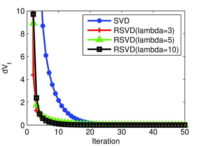
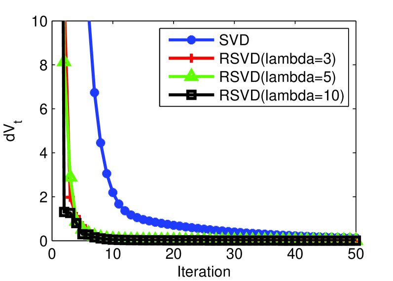
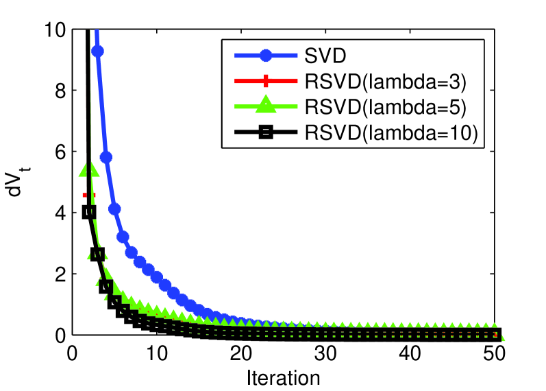
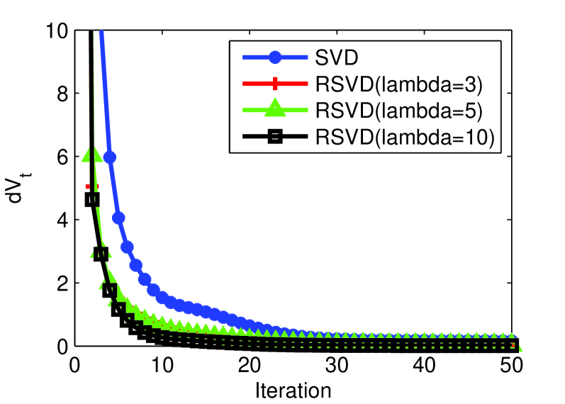
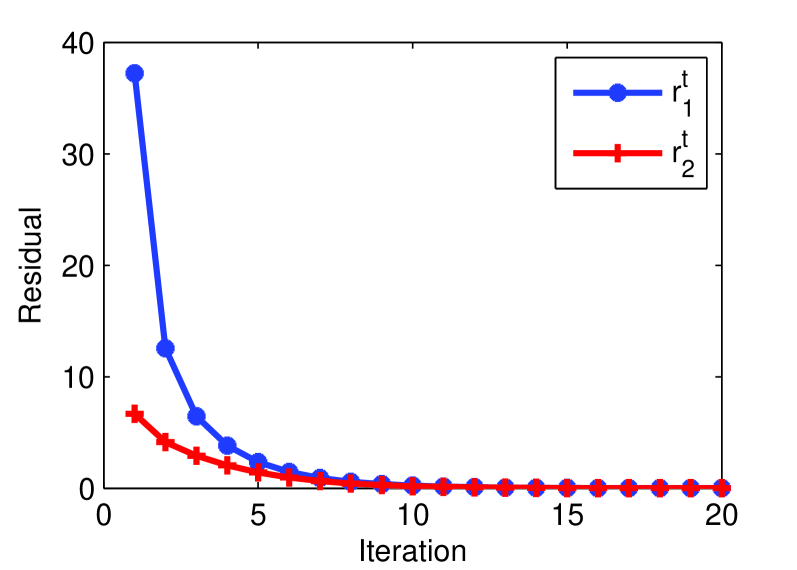
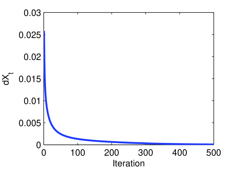
Convergence speed is important for a faster iterative algorithm. We will compare the convergence speed of RSVD with iterative SVD algorithm ($\lambda=0$). We define residual $dV_{t}$ to measure the difference of $V_{t}$ and $V_{t-1}$ in two consecutive iterations:

$$dV_{t}=\|V_{t}-V_{t-1}\|_{F},$$ (23)

where $t$ is the iteration number of Algorithm 2. We compare RSVD with SVD ($\lambda=0$) using different regularization weight parameter $\lambda=3,5,10$. Figure 1 shows the $dV_{t}$ decreases quickly along with iterations and RSVD converges faster than SVD.

6.4 RSVD share the same SVD subspace

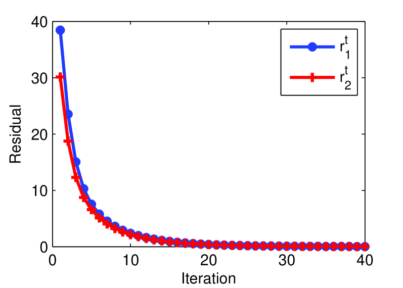
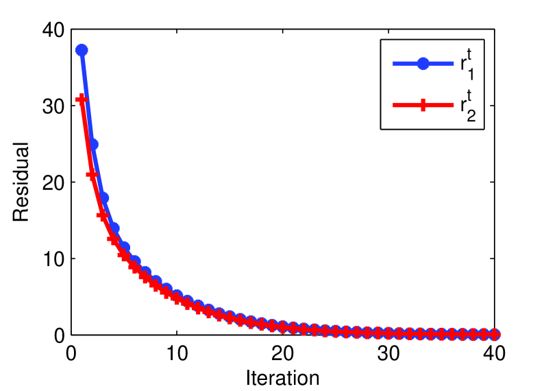
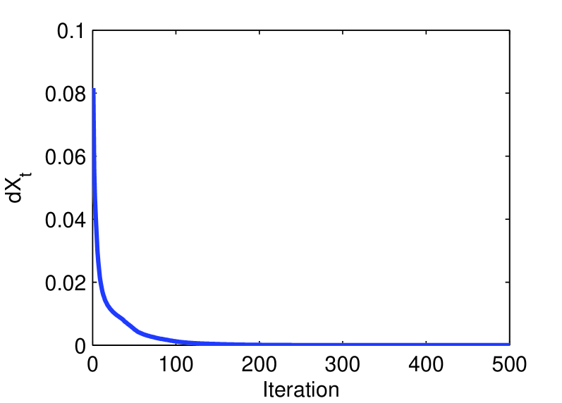
From Theorem 2, we know that the solution of RSVD should be in the subspace of SVD solution. Formally, let $U_{t},V_{t}$ be the solution of RSVD after $t$ iterations, $F,G$ be the solution of SVD, $X=FG^{T}$. We now introduce Eq.(24) and Eq.(25) to measure the difference between $U_{t},V_{t}$ and $F,G$. $r_{1}^{t}$ and $r_{2}^{t}$ are defined as

$$r_{1}^{t}=\|U_{t}-FA_{t}\|_{F}^{2},$$ (24)

$$r_{2}^{t}=\|V_{t}-GB_{t}\|_{F}^{2}.$$ (25)

In order to minimize $r_{1}^{t}$ and $r_{2}^{t}$, the solution of $A_{t}$ and $B_{t}$ can be given as:

$$A_{t}=(F^{T}F)^{-1}F^{T}U_{t},$$ (26)

$$B_{t}=(G^{T}G)^{-1}G^{T}V_{t}.$$ (27)

Substituting Eq.(26) and Eq.(27) back to Eq.(24) and Eq.(25), we get the minimized residual $r_{1}^{t}$ and $r_{2}^{t}$. If $r_{1}^{t}$ and $r_{2}^{t}$ are equal to $0$, it means that RSVD solution $U_{t}$ and $V_{t}$ share the same subspace as SVD solution $F$ and $G$. Figure 2 shows residual $r_{2}^{t}$ and $r_{3}^{t}$ converges to 0 after a few iterations.

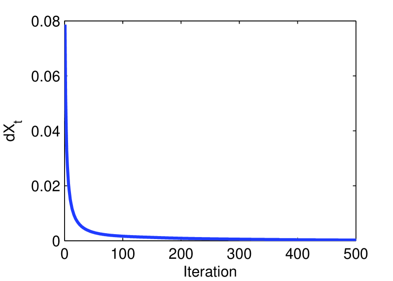
6.5 Convergence of recommender system solution

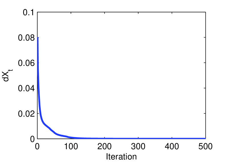
Solutions to the recommender systems Eqs.(19,20) converge. The EM-like algorithm has been shown effective in solving recommender systems srebro2003weighted koren2009matrix kurucz2007methods . We show the solution $(X_{t})_{\Omega}$ converges after $t$ iterations of EM-like iterations by using the difference,

$$dX_{t}=\frac{1}{\sqrt{N_{\Omega}}}\|X_{t}-X_{t-1}\|_{\Omega}.$$ (28)

where $N_{\Omega}$ is size of set $\Omega$. Figure 3 shows the experiment result of $dX_{t}$. As we can see, for all the 4 datasets, the solution converges in about 100 to 200 iterations.

6.6 Precision-Recall Curve

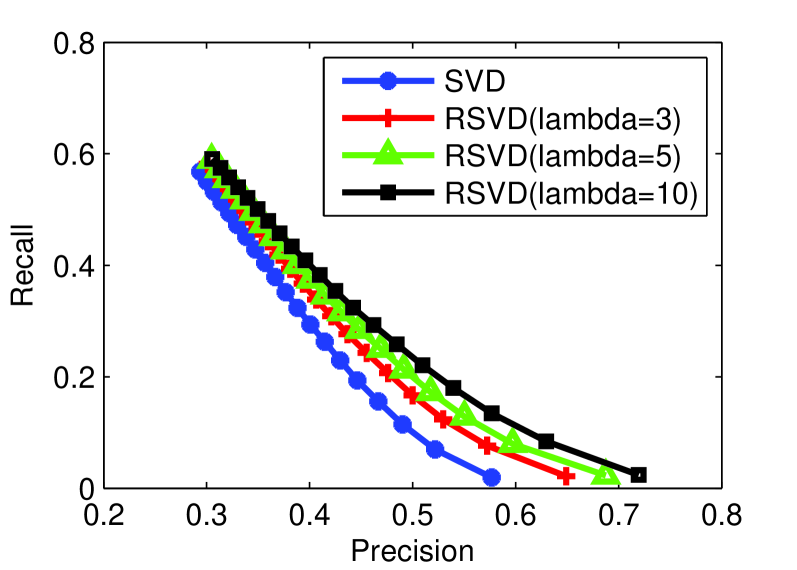
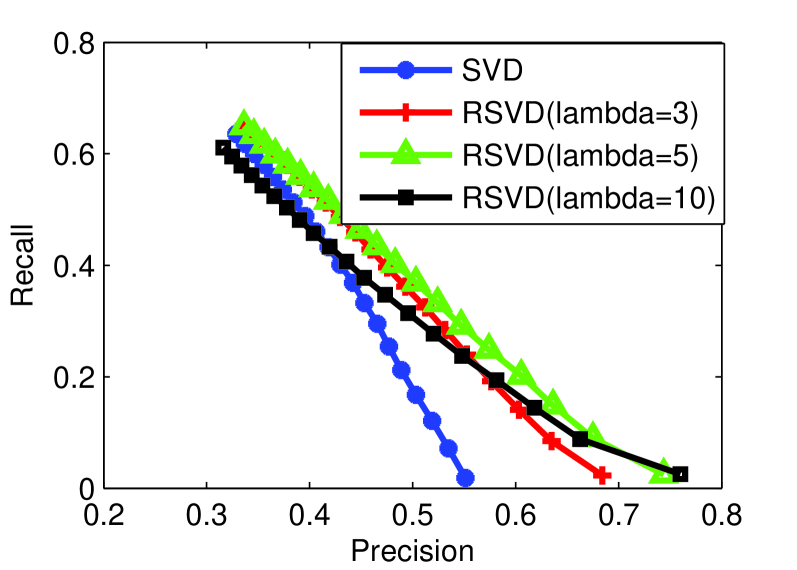
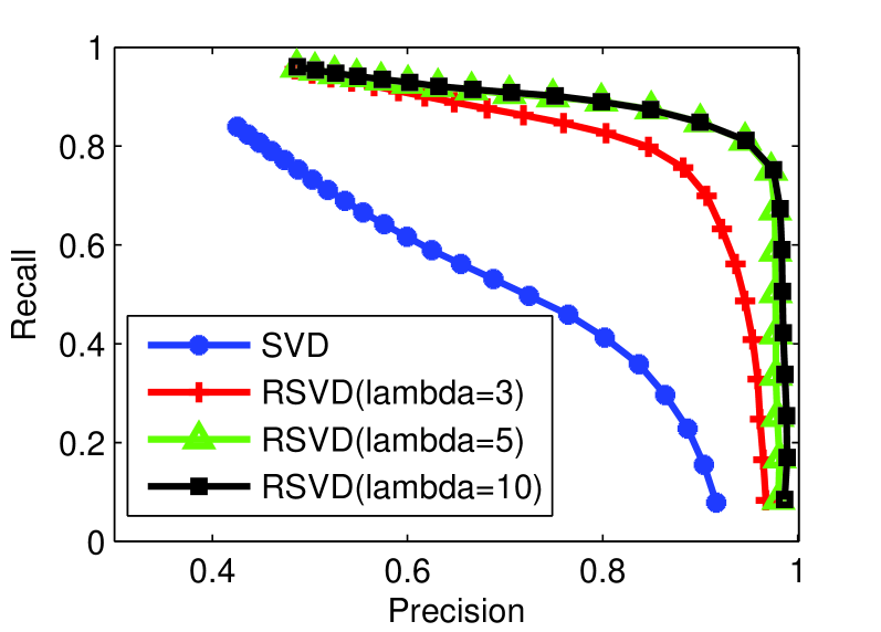
In this part, we compare the precision and recall of RSVD and SVD using different rank $k$ and regularization weight parameter $\lambda$. We use these $k$ and $\lambda$ settings because both RSVD and SVD models with these settings produce the best precision and recall. All the curves are the average results of 5 random run.

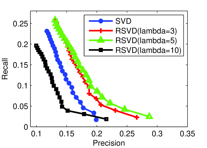
Figure 4 shows MovieLens data using SVD and RSVD with rank $k=3,5,7,9$. For each rank $k$, we compare SVD and RSVD with regularization weight parameter $\lambda=3,5,10$. As we can see, for each rank $k$, RSVD performs better than SVD generally. Choosing $\lambda$ properly could improve SVD algorithm and achieve the best precision and recall results.

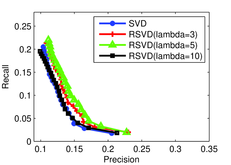
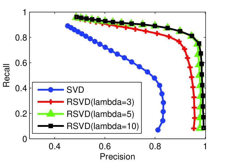
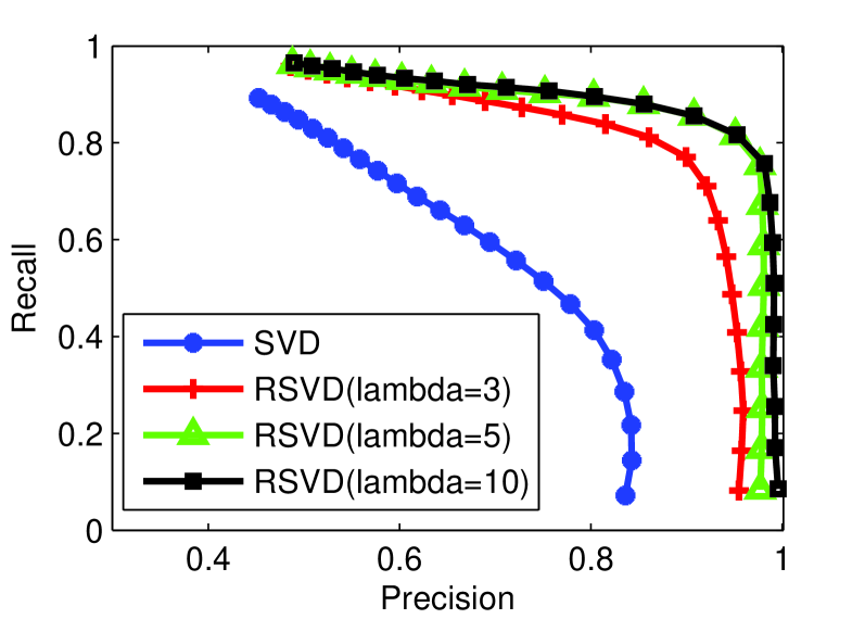
Figure 5 shows RottenTomatoes data using SVD and RSVD with rank $k=3,5,7,9$. In all figures, RSVD with $\lambda=5$ performs the best.

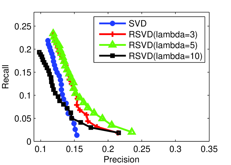
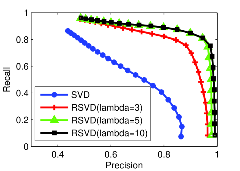
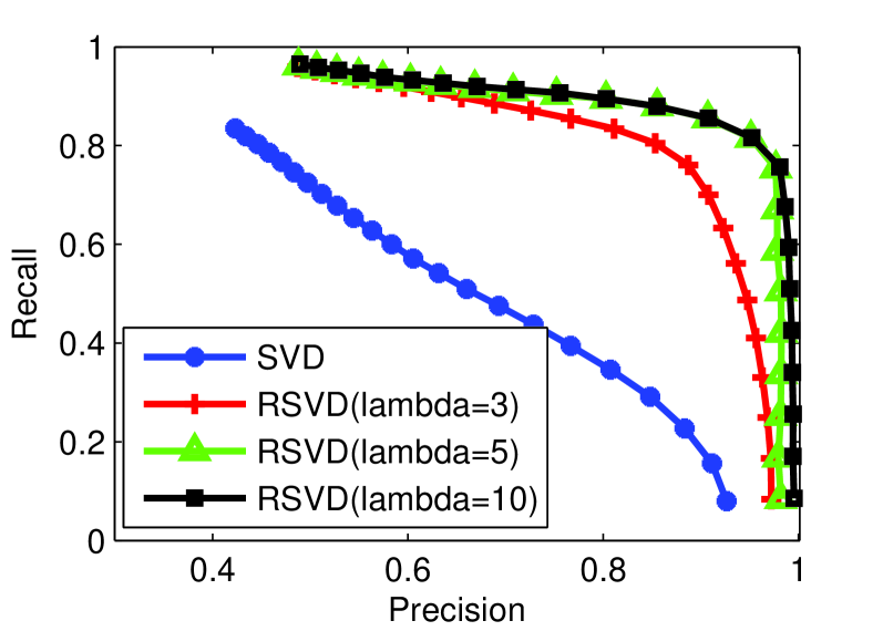
Figure 6 shows Jester1 data using SVD and RSVD with rank $k=14,16,18,20$. It is very easy to find that RSVD with $\lambda=5,10$ produce the best precision result for this data.

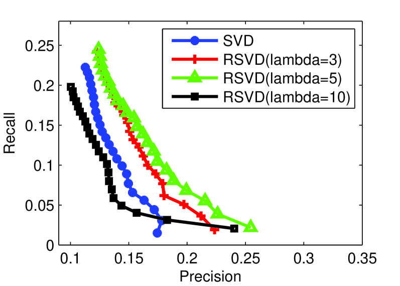
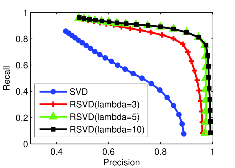
Figure 7 shows Jester2 data using SVD and RSVD with rank $k=14,16,18,20$. We can see from the results that RSVD with $\lambda=5,10$ produce the best precision result. As in Jester1 data, RSVD algorithm improves SVD significantly.

6.7 $F_{1}$ measure

$F_{1}$ measure combines precision and recall at the same time and can be used a good metric. $F_{1}$ measure is defined in Eq.(22). Since each $N$ gives a pair of precision and recall, we use $F_{1}$ measure when $N=n_{mask}$ as the standard. Because $N=n_{mask}$, if all the masked-out ratings are predicted correctly, the size of set $\mathbb{H}$ can be exactly $n_{mask}$, which means recall is 1. $F_{1}$ measure ranges from 0 to 1. A higher $F_{1}$ measure (close to 1) means that an algorithm has better performance.

Table 3 shows the $F_{1}$ measure of the four datasets. Each row denotes a dataset with a specific rank $k$. The best $F_{1}$ measure is denoted in bold. As we can see, for all the datasets and ranks that we experimented, $\lambda=5$ is a good setting that produces the highest $F_{1}$ measure. In all, RSVD performs much better than SVD in terms of $F_{1}$ measure. In applications, we can test different $\lambda$ and rank $k$ setting to find the best setting for specific problems.

Table 3: $F_{1}$ measure (best values are in bold.).

Data	SVD	RSVD	RSVD	RSVD
		($\lambda=3$)	($\lambda=5$)	($\lambda=10$)
MovieLens (k=3)	0.3700	0.3850	0.3922	0.4005
MovieLens (k=5)	0.3875	0.4100	0.4199	0.4232
MovieLens (k=7)	0.4152	0.4391	0.4439	0.4231
MovieLens (k=9)	0.4220	0.4497	0.4542	0.4244
RottenTomatoes (k=3)	0.1220	0.1308	0.1337	0.1235
RottenTomatoes (k=5)	0.1302	0.1413	0.1436	0.1176
RottenTomatoes (k=7)	0.1315	0.1501	0.1543	0.1228
RottenTomatoes (k=9)	0.1422	0.1614	0.1651	0.1240
Jester1 (k=14)	0.6587	0.8241	0.8668	0.8665
Jester1 (k=16)	0.6201	0.8151	0.8667	0.8659
Jester1 (k=18)	0.6188	0.8213	0.8672	0.8666
Jester1 (k=20)	0.6077	0.8177	0.8667	0.8658
Jester2 (k=14)	0.6506	0.8305	0.8730	0.8730
Jester2 (k=16)	0.6261	0.8277	0.8732	0.8725
Jester2 (k=18)	0.6114	0.8288	0.8729	0.8723
Jester2 (k=20)	0.5908	0.8259	0.8721	0.8722

7 Conclusion

In conclusion, SVD is the mathematical basis of principal component analysis (PCA). We present a regularized SVD (RSVD), present an efficient computational algorithm, and provide several theoretical analysis. We show that although RSVD is non-convex, it has a closed-form global optimal solution. Finally, we apply regularized SVD to the application of recommender system and experimental results show that regularized SVD (RSVD) outperforms SVD significantly.

References

- [1] O. Alter, P. O. Brown, and D. Botstein. Singular value decomposition for genome-wide expression data processing and modeling. Proceedings of the National Academy of Sciences, 97(18):10101–10106, 2000.
- [2] D. Billsus and M. J. Pazzani. Learning collaborative information filters. In ICML, volume 98, pages 46–54, 1998.
- [3] A. d’Aspremont, L. El Ghaoui, M. I. Jordan, and G. R. Lanckriet. A direct formulation for sparse pca using semidefinite programming. SIAM review, 49(3):434–448, 2007.
- [4] M. Deshpande and G. Karypis. Item-based top-n recommendation algorithms. ACM Transactions on Information Systems (TOIS), 22(1):143–177, 2004.
- [5] J. Friedman, T. Hastie, and R. Tibshirani. The elements of statistical learning, volume 1. Springer Series in Statistics New York, 2001.
- [6] K. Goldberg, T. Roeder, D. Gupta, and C. Perkins. Eigentaste: A constant time collaborative filtering algorithm. Information Retrieval, 4(2):133–151, 2001.
- [7] GroupLens. Grouplens research group. http://www.grouplens.org, 2014.
- [8] Y. Guan and J. G. Dy. Sparse probabilistic principal component analysis. In International Conference on Artificial Intelligence and Statistics, pages 185–192, 2009.
- [9] P. J. Hancock, A. M. Burton, and V. Bruce. Face processing: Human perception and principal components analysis. Memory & Cognition, 24(1):26–40, 1996.
- [10] J. L. Herlocker, J. A. Konstan, A. Borchers, and J. Riedl. An algorithmic framework for performing collaborative filtering. In Proceedings of the 22nd annual international ACM SIGIR conference on Research and development in information retrieval, pages 230–237. ACM, 1999.
- [11] IMDB. Imdb website. http://www.imdb.com, 2014.
- [12] I. Jolliffe. Principal component analysis. Wiley Online Library, 2005.
- [13] G. Karypis. Evaluation of item-based top-n recommendation algorithms. In Proceedings of the tenth international conference on Information and knowledge management, pages 247–254. ACM, 2001.
- [14] Y. Koren, R. Bell, and C. Volinsky. Matrix factorization techniques for recommender systems. Computer, 42(8):30–37, 2009.
- [15] M. Kurucz, A. A. Benczúr, and K. Csalogány. Methods for large scale svd with missing values. In Proceedings of KDD Cup and Workshop, volume 12, pages 31–38. Citeseer, 2007.
- [16] RottenTomatoes. Rotten tomatoes website. http://www.rottentomatoes.com, 2014.
- [17] B. Sarwar, G. Karypis, J. Konstan, and J. Riedl. Application of dimensionality reduction in recommender system-a case study. Technical report, DTIC Document, 2000.
- [18] B. Sarwar, G. Karypis, J. Konstan, and J. Riedl. Item-based collaborative filtering recommendation algorithms. In Proceedings of the 10th international conference on World Wide Web, pages 285–295. ACM, 2001.
- [19] H. Shen and J. Z. Huang. Sparse principal component analysis via regularized low rank matrix approximation. Journal of multivariate analysis, 99(6):1015–1034, 2008.
- [20] N. Srebro and T. Jaakkola. Weighted low-rank approximations. In ICML, volume 3, pages 720–727, 2003.
- [21] D. Williams, S. Zheng, X. Zhang, and H. Jamjoom. Tidewatch: Fingerprinting the cyclicality of big data workloads. In INFOCOM, 2014 Proceedings IEEE, pages 2031–2039. IEEE, 2014.
- [22] Y. Yang and X. Liu. A re-examination of text categorization methods. In Proceedings of the 22nd annual international ACM SIGIR conference on Research and development in information retrieval, pages 42–49. ACM, 1999.
- [23] X. Zhang, Z.-Y. Shae, S. Zheng, and H. Jamjoom. Virtual machine migration in an over-committed cloud. In Network Operations and Management Symposium (NOMS), 2012 IEEE, pages 196–203. IEEE, 2012.
- [24] Y. Zhang, A. d’Aspremont, and L. El Ghaoui. Sparse pca: Convex relaxations, algorithms and applications. In Handbook on Semidefinite, Conic and Polynomial Optimization, pages 915–940. Springer, 2012.
- [25] S. Zheng. Machine Learning: Several Advances in Linear Discriminant Analysis, Multi-View Regression and Support Vector Machine. PhD thesis, The University of Texas at Arlington, 2017.
- [26] S. Zheng, X. Cai, C. H. Ding, F. Nie, and H. Huang. A closed form solution to multi-view low-rank regression. In AAAI, pages 1973–1979, 2015.
- [27] S. Zheng and C. Ding. Kernel alignment inspired linear discriminant analysis. In Joint European Conference on Machine Learning and Knowledge Discovery in Databases, pages 401–416. Springer Berlin Heidelberg, 2014.
- [28] S. Zheng and C. Ding. Minimal support vector machine. arXiv preprint arXiv:1804.02370, 2018.
- [29] S. Zheng, F. Nie, C. Ding, and H. Huang. A harmonic mean linear discriminant analysis for robust image classification. In Tools with Artificial Intelligence (ICTAI), 2016 IEEE 28th International Conference on, pages 402–409. IEEE, 2016.
- [30] S. Zheng, K. Ristovski, A. Farahat, and C. Gupta. Long short-term memory network for remaining useful life estimation. In Prognostics and Health Management (ICPHM), 2017 IEEE International Conference on, pages 88–95. IEEE, 2017.
- [31] S. Zheng, Z.-Y. Shae, X. Zhang, H. Jamjoom, and L. Fong. Analysis and modeling of social influence in high performance computing workloads. In European Conference on Parallel Processing, pages 193–204. Springer Berlin Heidelberg, 2011.
- [32] S. Zheng, A. Vishnu, and C. Ding. Accelerating deep learning with shrinkage and recall. In Parallel and Distributed Systems (ICPADS), 2016 IEEE 22nd International Conference on, pages 963–970. IEEE, 2016.
- [33] H. Zou, T. Hastie, and R. Tibshirani. Sparse principal component analysis. Journal of computational and graphical statistics, 15(2):265–286, 2006.