Order-of-magnitude speedup for steady states and traveling waves via Stokes preconditioning in Channelflow and Openpipeflow

Abstract

Steady states and traveling waves play a fundamental role in understanding hydrodynamic problems. Even when unstable, these states provide the bifurcation-theoretic explanation for the origin of the observed states. In turbulent wall-bounded shear flows, these states have been hypothesized to be saddle points organizing the trajectories within a chaotic attractor. These states must be computed with Newton’s method or one of its generalizations, since time-integration cannot converge to unstable equilibria. The bottleneck is the solution of linear systems involving the Jacobian of the Navier-Stokes or Boussinesq equations. Originally such computations were carried out by constructing and directly inverting the Jacobian, but this is unfeasible for the matrices arising from three-dimensional hydrodynamic configurations in large domains. A popular method is to seek states that are invariant under numerical time integration. Surprisingly, equilibria may also be found by seeking flows that are invariant under a single very large Backwards-Euler Forwards-Euler timestep. We show that this method, called Stokes preconditioning, is 10 to 50 times faster at computing steady states in plane Couette flow and traveling waves in pipe flow. Moreover, it can be carried out using Channelflow (by Gibson) and Openpipeflow (by Willis) without any changes to these popular spectral codes. We explain the convergence rate as a function of the integration period and Reynolds number by computing the full spectra of the operators corresponding to the Jacobians of both methods.

1 Motivation and history

One of the fundamental properties of nonlinear systems is the existence of multiple solutions. Many, in fact, most of these are unstable and hence not accessible to time integration. Yet, they play a crucial role in organizing the solution sets and possibly the dynamics actually realized by the system. Bifurcation diagrams have long been studied in connection with classical hydrodynamic instabilities which form patterns, namely Taylor-Couette flow and Rayleigh-Bénard convection. In 1989, a method was formulated by Tuckerman tuckerman1989steady by which an explicit-implicit time integration code could be easily transformed to carry out steady state solving. More specifically, it was shown that taking the difference between successive widely spaced timesteps was equivalent to preconditioning the Jacobian with the inverse Laplacian or Stokes operator. This allowed the linear systems whose solution is required by Newton’s method to be solved economically by matrix-free iterative methods, which in turn allowed steady states in large systems ($O(10^{5})$–$O(10^{7})$ degrees of freedom) to be computed. This method, called Stokes preconditioning, was applied to calculate bifurcation diagrams in spherical Couette flow by Mamun & Tuckerman mamun1995asymmetry , convection in Cartesian xin1997natural ; xin2002extended ; xin2012stability ; chenier1999stability ; mercader2005bifurcations ; henry2007multiple ; dridi2008influence ; torres2013three ; torres2014bifurcation ; torres2015transition , cylindrical touihri1999onset ; touihri2011instabilities ; assemat2007nonlinear ; marques2007centrifugal ; boronska2010extreme ; mercader2014secondary ; sanchez2016natural and spherical bergemann2008geoflow ; feudel2011convection ; feudel2013multistability ; feudel2015bifurcations ; feudel2017hysteresis geometries by researchers such as Xin, Chenier, Henry, and Feudel, to von Kármán flow daube2002numerical ; nore20031 ; nore2004survey by Daube, Nore, and Le Quéré and to Bose-Einstein condensation huepe1999decay ; abid2003gross by Huepe, Brachet and co-workers

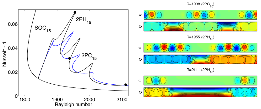
One of the problems to which Stokes preconditioning has been applied most extensively is that of double diffusive convection xin1998bifurcation ; bergeon1998marangoni ; bergeon1999double ; bardan2000nonlinear ; bergeon2002natural ; bergeon2003soret ; meca2004blue ; meca2004complex ; mercader2004numerical ; batiste2004hydrodynamic ; alonso2005numerical ; alonso2007complex . In 2006, a comprehensive theory of localized states via homoclinic snaking was developed by Knobloch and co-workers burke2006localized , following earlier ideas by Champneys, Coullet, Fauve, Pomeau and others champneys1998homoclinic ; coullet2000stable ; fauve1990solitary ; pomeau1986front ; m1995pattern . This theory predicts and explains the existence of a large number of branches linked by saddle-node bifurcations and thus spotlights the crucial role of unstable steady states and their computation. The first instances of localized states and homoclinic snaking in realistic physical systems were computed in 2006–8 by researchers such as Alonso, Assemat, Batiste, Bergeon, and Mercader batiste2006spatially ; alonso2007numerical ; bergeon2008spatially ; bergeon2008periodic ; assemat2008spatially , all for double diffusive convection and all using the Stokes preconditioning method, followed by further studies of these phenomena by Beaume, LoJacono and others lo2010spatially ; beaume2011homoclinic ; mercader2011convectons ; beaume2013convectons ; beaume2013nonsnaking ; mercader2013travelling ; jacono2017spatially ; jacono2017localized ; jacono2017complex . In the Appendix, we will show examples of the more exotic or interesting bifurcation diagrams that have been calculated by various groups using the Stokes preconditioning method.

The cases studied above involved flows which undergo linear instabilities from a homogeneous state, leading to patterns. We now turn to shear flows confined between rigid or free-slip boundaries, namely plane Couette flow, plane Poiseuille flow and pipe flow, which are linearly stable over the parameter range of interest. In 1990, Nagata Nagata1990three computed the first non-trivial steady state for plane Couette flow; this was followed by computations of other steady states and traveling wave solutions for plane Couette and Poiseuille flow by Waleffe waleffe1998three ; waleffe2001exact ; waleffe2003homotopy who coined the term Exact Coherent Structure (ECS) to describe unstable steady states, traveling waves, periodic orbits, and other low-dimensional dynamically relevant invariant solutions with low-dimensional unstable manifolds in these shear flows. These and other contemporaneous computations clever1997tertiary ; nagata1997three ; faisst2000transition ; Schmiegel_PhD used dedicated steady-state codes in which the Jacobians were constructed and the linear systems required by Newton’s method were solved directly. Many used homotopy to modify steady states or traveling waves already known to exist in convection or in Taylor-Couette flow. In 2003–4, the first traveling waves in pipe flow were computed by Eckhardt, Kerswell and co-workers faisst2003traveling ; wedin2004exact , also using Jacobian matrices and direct matrix inversion. All of these solutions were computed in small periodic domains or minimal flow units, which are the smallest domains in which turbulence can be maintained. The motivation for these searches was provided by Cvitanović and Eckhardt cvitanovic1991periodic ; Cvitanovic_Eckhardt and by Kawahara kawahara2001periodic ; kawahara2012significance . Building on previous ideas by Smale, Ruelle, Bowen and Sinai, the authors proposed that turbulence could be viewed from a deterministic dynamical systems perspective as a collection of trajectories ricocheting between ECSs along their unstable directions.

Influential work on numerical methods dennis1996numerical ; knoll2004jacobian ; sanchez2004newton ; viswanath2007recurrent ; van2011matrix by authors such as Sánchez, Net, van Veen, Viswanath, and others led to the adoption of iterative matrix-free methods and to many additional solutions pringle2007asymmetric ; kerswell2007recurrence ; duguet2008transition ; duguet2008relative ; gibson2008visualizing by reseachers such as Duguet, Gibson, Halcrow, Pringle and Willis. Catalogs of solutions computed by 2009 were given in Schmiegel_PhD ; gibson2009equilibrium ; pringle2009highly . In a development parallel to what was happening at the same time in double diffusive convection, focus was extended from the minimal flow unit to localized and snaking solutions. Since these consist of one or more active regions surrounded by possibly wide quiescent regions, computations of localized states are far more costly. The codes Channelflow gibson2008visualizing ; channelflow by Gibson and Openpipeflow willis2017openpipeflow by Willis took advantage of the matrix-free iterative approach to treat larger domains, leading to the discovery of localized states in plane Couette flow by Schneider et al. schneider2010snakes in 2010 and in pipe flow by Avila et al. avila2013streamwise in 2013, followed by many others gibson2014spanwise ; brand2014doubly ; eckhardt2014doubly ; chantry2014genesis . Mellibovsky and Eckhardt mellibovsky2011takens used Stokes preconditioning to investigate a Takens-Bogdanov scenario for travelling waves in pipe flow. Beaume and co-workers beaume2015reduced ; beaume2016modulated used the method to calculate ECSs for an asymptotic reduction of the free-slip version of plane Couette flow called Waleffe flow waleffe1998three ; waleffe2001exact ; waleffe2003homotopy and were able to reproduce the high-Reynolds-number scaling calculated in wang2007lower ; blackburn2013lower ; deguchi2014high .

The primary purpose of this Chapter is to compare the method used in Channelflow and Openpipeflow with the Stokes preconditioning method. We show that the Stokes preconditioning method can be carried out by using the options already present in Channelflow and Openpipeflow without any changes to the codes themselves. The user must simply liberate him or herself from standard notational convention and allow the timestep $\Delta t$ to approach infinity, as will be explained in Section 2. In Section 3, we will give examples of steady states and traveling waves calculated by Channelflow and Openpipeflow using the Stokes preconditioning method. We will show that these computations are up to 50 times faster than when they are carried out via the classical approach previously used by Channelflow and Openpipeflow, emphasizing again that this is accomplished only by the choice of different parameters.

2 Stokes preconditioning

We begin with the schematically written differential equation, or dynamical system:

$$\frac{\partial U}{\partial t}=LU+N(U),$$ (1)

for a flow-field $U$, where $L$ stands for the linear terms, typically the viscous or diffusive terms in hydrodynamics and $N$ for the nonlinear terms, typically the advective terms. We seek steady states of (1), i.e. roots of $L+N$, or $U$ such that

$$0=LU+N(U).$$ (2)

There are other ways to define steady states. In particular, we may seek

$$0=U(T)-U(0)\equiv(\Phi_{T}-I)U(0),$$ (3)

where $U(T)$ is computed from $U(0)$ by time-integration of (1), and where $\Phi_{T}$ is the operator which takes an initial condition $U(0)$ to the field $U(T)$ at time $T$. We note that, in addition to equilibria, definition (3) is satisfied by $T$-periodic orbits of the dynamical system, which we will not consider here.

In practice, temporal integration of nonlinear evolution equations cannot be carried out exactly. A notable exception to this, useful for conceptual purposes, is if $N$ is in fact linear, so that we may write

$$U(T)=e^{(L+N)T}U(0).$$ (4)

In general, however, $\Phi_{T}$ must be approximated as the product of many small approximate timesteps. That is,

$$\Phi_{T}\approx\left(B_{\Delta t}\right)^{T/\Delta t},$$ (5)

where $B_{\Delta t}$ is a numerical timestepping operator with step size $\Delta t$. One straightforward approach combines backward-Euler timestepping for $L$ with forward-Euler timestepping for $N$, leading to the BEFE algorithm

$$B_{\Delta t}\equiv(I-\Delta tL)^{-1}(I+\Delta tN),$$ (6)

which is used in the Stokes preconditioning method.

Despite the use of the notation $L$ and $N$, the necessary distinction is actually between the implicitly and explicitly integrated parts of the operator; although $L$ must be linear, $N$ may include some of the linear terms. In the interests of keeping the notation simple, we will not always be rigorous about distinguishing between an operator such as $N$ and its linearization $N_{U}$ about a solution $U$. We will also not distinguish between the spatially continuous equations and their spatially discretized versions. Nor will we consider the constraints, i.e. boundary conditions, incompressibility, and the crucial related question of determination of the pressure, assuming the constraints to be incorporated into the implementation of $(I-\Delta tL)^{-1}$, although we will later briefly address these questions.

We make a few comments about (6). First, the expression $(I-\Delta tL)^{-1}$ should be understood as making a rational approximation to $e^{\Delta tL}$, called implicit, meaning in this case that it requires an operator inversion. The expression $(I+\Delta tN)$ should be understood as a polynomial approximation to $e^{\Delta tN}$ and is called explicit because it requires only operator actions. The reason for which $L$ is integrated implicitly is that it has widely spaced eigenvalues, a property called stiffness in the context of differential equations. Stiffness implies that a polynomial (explicit) approximation of the exponential would require unacceptably small $\Delta t$ in order to remain finite. The polynomial approximation $(I+\Delta tN)$ also limits the size of $\Delta t$, but far less than the limitation that would be imposed by the explicit integration of $L$. It is very fortunate that it is the linear term $L$ that bears most of the responsibility for the stiffness of (1), since implicit formulas involving the nonlinear term $N$ would be much harder to evaluate, requiring Newton iteration at each timestep, rather than merely the inversion of a linear operator. Hence, mixed explicit-implicit formulas such as (6) are almost universally used in hydrodynamics.

For small $\Delta t$, the Taylor expansion of (6) shows that

$$B_{\Delta t} \equiv (I-\Delta tL)^{-1}(I+\Delta tN)$$ (7)

$$\approx (I+\Delta tL+(\Delta tL)^{2}+\ldots)(I+\Delta tN)$$

$$\approx I+\Delta t(L+N)+\Delta t^{2}(L^{2}+LN)+\ldots$$

while (4) shows that the exact flow satisfies

$$\Phi_{\Delta t}=I+\Delta t(L+N)+\Delta t^{2}(L+N)^{2}/2+\ldots$$ (8)

Thus, (6) is first-order accurate, meaning that the Taylor series agree to order $\Delta t$. Note that the disagreement between (7) and (8), here at order $\Delta t^{2}$, is not a function of $L+N$, a property called time-splitting error. Other, more accurate, timestepping operators may be used instead of BEFE to approximate $\Phi_{T}$, but time-splitting errors are always present when different formulas are used to integrate $L$ and $N$.

Let us now calculate the increment produced by evolving with the Backwards-Euler Forwards-Euler method (6) over a single timestep:

$$B_{\Delta t}-I = (I-\Delta tL)^{-1}(I+\Delta tN)-I$$ (9)

$$= (I-\Delta tL)^{-1}\left[(I+\Delta tN)-(I-\Delta tL)\right]$$

$$= (I-\Delta tL)^{-1}\Delta t(L+N).$$

We emphasize that, unlike (7), equation (9) is an exact algebraic calculation and not a Taylor expansion: it is valid for all values of $\Delta t$. Thus, (9) demonstrates the simple and powerful result that roots of $B_{\Delta t}-I$ are also exact roots of $L+N$, regardless of the value of $\Delta t$. Equation (9) follows from the definition (6) of the BEFE algorithm: it is not a general property of timestepping schemes.

We recall that a wide distribution of eigenvalues of an operator is called stiffness in the context of differential equations; the same property is called poor conditioning in the context of linear operators. Poor conditioning can be counteracted by preconditioning, i.e. multiplication by an operator which resembles the inverse of the poorly conditioned operator, but whose action is more easily or cheaply carried out. Thus, (9) shows that $B_{\Delta t}-I$ is a version of $L+N$ that has been preconditioned by $(I-\Delta tL)^{-1}$. Since, in the hydrodynamic context, $\partial U/\partial t=LU$ is the time-dependent Stokes (rather than Navier-Stokes) equation, for which $(I-\Delta tL)^{-1}$ is the (implicit) timestepping operator, we call this Stokes preconditioning.

In the limit of small $\Delta t$, we have

$$(B_{\Delta t}-I)=(I-\Delta tL)^{-1}\Delta t(L+N)\approx\Delta t(L+N),$$ (10)

while in the limit of large $\Delta t$, we have

$$(B_{\Delta t}-I)=(I-\Delta tL)^{-1}\Delta t(L+N)\approx-L^{-1}(L+N).$$ (11)

Varying $\Delta t$ interpolates between these two cases, that of $L+N$ preconditioned by $L^{-1}$ and that of $L+N$ itself. (The conditioning or stiffness of operators is unaffected by scalar multiplication, since it is the ratio between eigenvalues or timescales that is significant.) We emphasize that Stokes preconditioning is not carried out as a separate operation: that is, we do not apply $L+N$ followed by $(I-\Delta tL)^{-1}$. Instead, we carry out $B_{\Delta t}-I$, which (9) shows to be equivalent to the product of these two operators. In what follows, we will write $B_{T}-I$, keeping in mind that $T$ may be of any size.

We summarize what we have said above by defining various nonlinear operators $G$ whose roots are the exact, or approximate, steady states of (1). We define two theoretical operators:

$$G^{\rm rhs} \equiv L+N,$$ (12)

$$G^{\rm flow}=G^{\rm flow}_{T} \equiv \Phi_{T}-I,$$ (13)

whose roots are steady states of the underlying dynamical system (1), in accordance with the definitions given in (2) and (3) respectively. These roots may be computed by seeking the zeros of the following two numerical operators, whose comparison will be the main focus of this Chapter:

$$G^{\rm Stokes}=G^{\rm Stokes}_{T} \equiv B_{T}-I,$$ (14)

$$G^{\rm int}=G^{\rm int}_{T} \equiv \left(B_{\Delta t}\right)^{T/\Delta t}-I.$$ (15)

We omit the time $T$ when it is not important.

These two operators are fundamentally different. Unlike $G^{\rm int}$, $G^{\rm Stokes}$ is not a time-discretized version of $G^{\rm flow}$. Instead, as shown in (9), the roots of $G^{\rm Stokes}$ are those of $G^{\rm rhs}$ if BEFE is used for $B_{T}$. This is true for any value of $T$, but only a large value of $T$ leads to a well-conditioned Jacobian. In contrast, $G^{\rm int}$ corresponds to standard time-integration of $G^{\rm flow}$. Although any scheme including BEFE may be used, typically higher-order methods, such as Crank-Nicolson Adams-Bashforth or semi-implicit Runge-Kutta are preferred. For $G^{\rm int}$ to approximate $G^{\rm flow}$, $\Delta t$ must have a small value in order for the time integration to be accurate and stable. With the usual non-dimensionalization of space and time, and at Reynolds or Rayleigh numbers in the pattern-forming or transitional range, this usually means $\Delta t=O(0.01)$. Despite their very different natures, the coding for the two operators is identical. The difference is only quantitative: for $G^{\rm Stokes}$, one BEFE timestep is taken, with $\Delta t=T$ large, while for $G^{\rm int}$, many timesteps with small $\Delta t$ are taken.

Steady states, i.e. roots of an operator $G$, are calculated via Newton’s method. For an estimated steady state $U$, we write the linear approximation to $G$

$$G(U-u)\approx G(U)-G_{U}u,$$ (16)

where $G_{U}$ is the linearization of $G$ about $U$ and select $u$ such as to make the right-hand-side of (16) zero:

$$G_{U}u=G(U),$$ (17)

updating $U$ as

$$U\leftarrow U-u.$$ (18)

Traveling waves can be considered to be steady states in a moving frame. Rather than $\partial U/\partial t=0$, waves traveling in the $x$-direction satisfy

$$\frac{\partial U}{\partial t}=-C\frac{\partial U}{\partial x},$$ (19)

where the wavespeed $C$ is an additional unknown. Therefore, they may be computed as steady states of

$$0=LU+N(U)+C\frac{\partial U}{\partial x},$$ (20)

by adding $C\partial U/\partial x$ to the operator $N$ and imposing an additional condition to fix the spatio-temporal phase of the traveling wave.

The bottleneck for Newton’s method is the solution of the linear system (17). Assuming that the dimension of $G_{U}$ is too large for (17) to be solved directly via Gaussian elimination, it must be solved iteratively using a matrix-free approach that avoids explicit construction of the Jacobian. The method of choice is conjugate gradient iteration or, rather, one of its suitable generalizations for non-symmetric positive definite operators $G_{U}$. The most widely used of these is GMRES, Generalized Minimum RESidual saad1986gmres , but BiCGSTAB van1992bi also has its adherents. These methods calculate an approximation to $u$ in a Krylov space, i.e. in the space spanned by successive actions of the linear operator $G_{U}$ on $G(U)$:

$$G(U),\;G_{U}\,G(U),\;G_{U}^{2}\,G(U),\;\ldots\;G_{U}^{k}\,G(U),\;\ldots\;G_{U}^{K-1}\,G(U).$$ (21)

The CPU time required to solve (17) thus depends on two factors:

$$\mbox{--the time required for a single action by $G_{U}$},\qquad\qquad\qquad\qquad\qquad\qquad\qquad$$

    determined by the number of timesteps $$T/\Delta t$$, and (22)

–the number $$K u$$ of actions needed to approximate the solution ,

    determined by the conditioning of $$G_{U}$$. (23)

The action of $G_{U}$ on $u$ can be carried out by taking $N\rightarrow N_{U}$, i.e. substituting

$$(\mathbf{U}\cdot\nabla)\mathbf{U}\rightarrow(\mathbf{u}\cdot\nabla)\mathbf{U}+(\mathbf{U}\cdot\nabla)\mathbf{u}$$ (24)

and replacing all inhomogeneous terms such as boundary conditions, pressure gradients or fluxes, by corresponding homogeneous terms. This can typically be accomplished with very little modification to a code. Alternatively, it can be approximated via finite differences as

$$[G(U+\epsilon u)-G(U)]/\epsilon$$ (25)

In either case, evaluation of $G_{U}u$ typically takes approximately the same time as evaluation of $G(U)$. Therefore the time required to compute one such action is proportional to the number of timesteps $T/\Delta t$. For an optimized pseudospectral code, the most time-consuming portion of a timestep is spent in the spectral-to-physical transforms, which take a time roughly proportional to

$$M_{x}M_{y}M_{z}\left(\log M_{x}+\log M_{y}+\log M_{z}\right)\equiv M\log M,$$ (26)

where $M_{x},M_{y},M_{z}$ are the number of gridpoints or modes in each of the three Cartesian directions and $M$ is their product. For finite-difference discretizations, the most time-consuming portions may be the inversion of elliptic operators, which in tensor-product geometries can be carried out tuckerman1989steady ; lynch1964direct ; haidvogel1979accurate ; vitoshkin2013direct in a time proportional to

$$M_{x}M_{y}M_{z}\left(M_{x}+M_{y}+M_{z}\right)\sim M^{4/3}.$$ (27)

We will consider that the CPU time spent in carrying out actions by $G_{U}$ is proportional to $K\;(T/\Delta t)\;M^{1+\alpha}$ with $0\leq\alpha\leq 1$. The number $K$ of actions is determined by the nature of the operator $G_{U}$, more specifically its spectrum, a simple measure of which is given by its condition number, which is roughly the ratio of absolute values of the largest to the smallest eigenvalue. The total number of timesteps taken in each Newton step is the product $K\times T/\Delta t$.

Other considerations can enter into the timing. The most important one we have found is related to the GMRES algorithm without restarts, which requires the orthogonalization of all of the Krylov vectors (21) to each other, requiring $K(K-1)/2$ scalar products of vectors of length proportional to $M$. For $K$ sufficiently large, the CPU time required to take these scalar products may approach or even exceed that taken by the timesteps. We may write the total time required to take one Newton step as

$${\rm CPU}\approx c_{\rm action}\frac{T}{\Delta t}KM^{1+\alpha}+c_{\rm orth}K^{2}M,$$ (28)

where $c_{\rm action}\gg c_{\rm orth}$ are prefactors measuring the CPU time taken to perform a timestep or a scalar product.

3 Stokes preconditioning using Channelflow and Openpipeflow

We have carried out computations of steady states in plane Couette flow using Channelflow and traveling waves in pipe flow using Openpipeflow. In the plane Couette case, the computations using the Stokes preconditioning method take about 10% of the time required by computations using the classic integration method when measured in terms of number of timesteps required. For pipe flow, the Stokes preconditioning method is 35 to 50 times faster than the classic integration method. This section gives details of these computations and explores the conditioning properties of the operators $G^{\rm Stokes}$ and $G^{\rm int}$.

3.1 The flows

The mathematical framework for plane channel flows assumes flow between infinite parallel plates, with velocities which are prescribed on the plates and which are assumed periodic in the two directions parallel to the plates. Each periodic boundary condition must be completed by specifying either the flux or the pressure gradient in that direction. Plane Couette flow prescribes a finite velocity difference between the plates and no pressure gradient in the directions parallel to the plates, while standard plane Poiseuille flow prescribes no velocity difference between the plates, a finite pressure gradient or flux in one parallel direction and zero flux in the other. The direction between the plates is called cross-channel or wall-normal, the direction of the fixed velocity difference in the Couette case or of the fixed pressure gradient or flux in the Poiseuille case is called streamwise and the remaining direction is called spanwise. (Any combination of Poiseuille and Couette flow is possible and, in addition, the flux can be chosen to be zero in either flow by the appropriate choice of velocity at the walls.) Pipe flow, in a cylindrical geometry, also has two periodic directions, with a prescribed velocity on the pipe surface, a pressure gradient or flux in the streamwise direction and zero pressure gradient in the azimuthal direction.

Although the three flows are qualitatively different, their overall behavior is extremely similar. All have simple laminar states which are homogeneous in the periodic directions, All undergo transition to turbulence despite the fact that the laminar states are linearly stable in the Reynolds number range relevant for transition. (Plane Couette flow and pipe flow are linearly stable for all Reynolds numbers, while plane Poiseuille flow becomes unstable for a Reynolds number which is considerably higher than that at which transition takes place.) All possess an abundance of unstable states, which we investigate below. Two differences are relevant for our discussion. First, when there is an imposed flux (or pressure gradient) along the streamwise direction of the pipe or channel, states which break the streamwise homogeneity are not steady, but traveling waves or more complex flows. Second, the Reynolds numbers defined for the three flows use different conventions. Since for all of these flows the instability mechanism is shear, a common Reynolds number based on a single-sign shear layer would be more appropriate. Laminar plane Couette flow ($U_{\rm lam}=y$ over $-1\leq y\leq 1$) possesses one single-sign shear layer with $\Delta U=2$ and $\Delta Y=2$, while the $y=0$ plane divides laminar plane Poiseuille flow ($U_{\rm lam}=3(1-y^{2})/2$ over $-1\leq y\leq 1$) into two opposite-sign shear layers each with $|\Delta U|=3/2$ and $\Delta Y=1$, which yields a factor of $4/(3/2)=8/3=2.67$ between the conventional Reynolds numbers for Couette and Poiseuille flow. For pipe flow ($U_{\rm lam}=2(1-4r^{2})$ over $0\leq r\leq 1/2$) the length scale used in defining the Reynolds number is the diameter, so that $\Delta U=2$ and $\Delta Y=1/2$. Hence the conventional Reynolds numbers for pipe flow are roughly four times those for plane Couette flow with similar phenomenology. Evidence for this is that transition to turbulence begins in plane Couette flow at $Re\sim 325$ shi2013scale , in plane Poiseuille flow at $Re\sim 1000$, and in pipe flow at $Re\sim 2040$ avila2011onset , a factor of 6.3 higher than for transition in plane Couette flow. The lowest known non-trivial states appear at 127 for plane Couette flow clever1997tertiary ; waleffe2003homotopy and at 773 for pipe flow pringle2009highly , a factor of 6.

3.2 The codes

The Channelflow gibson2008visualizing ; channelflow and Openpipeflow willis2017openpipeflow software packages are widely used in the hydrodynamic stability community. As their names imply, Channelflow and Openpipeflow simulate flows in a planar and in a cylindrical geometry, respectively. Both treat tensor-product geometries, with two periodic directions and one non-periodic direction. Both represent the two periodic directions as Fourier series, taking derivatives in the Fourier space, where they are sparse. This means that inverting Laplacian ($L$) and Helmholtz ($I-\Delta tL$) operators is cheap and easy: these inversions are carried out exactly and not iteratively, contrary to what is done in spectral element or finite volume codes meant to treat general geometries. Both use the influence matrix technique to impose incompressibility so that the solutions calculated are divergence-free to machine accuracy and not merely to some power of $\Delta t$. In addition to timestepping, i.e. action by $B_{\Delta t}$, both have also implemented steady-state solving, using Newton’s method to find roots of $G^{\rm int}$. It can be seen from (14) and (15) that the operator $G^{\rm Stokes}$ can be represented via $G^{\rm int}$ merely by setting the parameters $T$ and $\Delta t$ to be equal and selecting the BEFE scheme to perform the timestepping, rather than the higher order methods that are usually preferred for evaluation of $G^{\rm int}$. No changes at all need to be made to the codes, which makes them ideal for comparing the calculation of steady states and traveling waves via $G^{\rm int}$ versus $G^{\rm Stokes}$.

We complete the description of the two codes by mentioning a few other elements which are less relevant for our purpose. Channelflow discretizes the spatial derivatives in the direction between the two bounding planes via Chebyshev polynomials, while Openpipeflow discretizes the nonperiodic radial direction via finite differences. Both codes use a Chebyshev grid spacing in the nonperiodic direction, with points concentrated near the solid boundaries. Both use the pseudospectral method, with derivatives taken in the Fourier space and multiplications carried out by transforming to a gridspace representation, multiplying the values at each point and then transforming back. Both use GMRES to solve the linear systems (17). Both approximate the action of $G_{U}$ as a difference (25) between two actions of $G$. Both implementations improve the convergence radius of Newton’s method by including the complementary hookstep viswanath2007recurrent feature, which constrains the Newton step so that it remains within a trusted region of validity for linearization (16).

3.3 Computations with Channelflow

Figure 1: Visualization of the steady state EQ1, also called NCBW. Left: Cutaway perspective view. Colors show streamwise velocity, arrows show velocity in various planes. Right: Streamwise cross-section showing deviation of streamwise velocity from the laminar state. Adapted from Gibson, Halcrow, Cvitanović gibson2009equilibrium .

Figure 2: Performance of Newton’s method with GMRES in Channelflow for single-step Stokes preconditioning method $G^{\rm Stokes}_{T}$ and for multi-step integration method $G^{\rm int}_{T}$ for various values of $T$. The initial condition is the steady EQ1 state Nagata1990three ; clever1997tertiary ; waleffe1998three ; waleffe2003homotopy at $Re=400$ and $Re$ is lowered to 380. Ordinate shows $\log||G(U)||$ at each Newton iteration, while abscissa shows the number of timesteps taken thus far. Each curve is labelled by its value of $T$. Left: Performance of single-step $G^{\rm Stokes}_{T}\equiv B_{T}-I$. Convergence is fastest when $T$ is highest, achieving approximately asymptotic performance for $T=100$ (solid curve). Right: Performance of multi-step $G^{\rm int}_{T}\equiv(B_{\Delta t})^{T/\Delta t}-I$ with timestep $\Delta t=0.031\,25$. Convergence is fastest when $T$ is lowest, achieving approximately asymptotic performance for $T=1$ (solid curve). Shown for comparison is the convergence curve for $G^{\rm Stokes}$ with $T=100$. Short black lines highlight the difference in speed between the two methods: the classic integration method takes 9500 timesteps in this case, while the Stokes method takes 860 timesteps, a ratio of 11.

Figure 3: Left: Dependence of the number $K$ of GMRES iterations (hollow circles) required for convergence for a typical Newton step as a function of $T$, plotted along with the number $T/\Delta t$ of timesteps (crosses) per action of the operator. As $T$ increases, the number $T/\Delta t$ of timesteps required per action obviously increases, while the $K$ required by $G^{\rm int}$ (hollow circles) decreases from 152 to 7, showing that its condition number improves. In contrast, for $G^{\rm Stokes}$, $T/\Delta t=1$ but the $K$ required is much larger, decreasing with $T$ and saturating at around 230 for $T\gtrsim 10$. Circles containing crosses shows $\log(K)+\log(T/\Delta t)=\log(KT/\Delta t)$, the log of the total number of timesteps in a typical Newton step. Right: Convergence during the solution of linear equations for four successive Newton steps at $Re=500$ for $G^{\rm int}_{T=1}$ and for $G^{\rm Stokes}_{T=100}$. For each curve, convergence is interrupted by plateaus. The linear system involving $G^{\rm int}$ requires fewer actions with $G_{U}$ than $G^{\rm Stokes}$, a consequence of the fact that $G^{\rm int}$ is better conditioned than $G^{\rm Stokes}$. The number $K$ of actions required by $G^{\rm Stokes}$ increases at each successive Newton step.

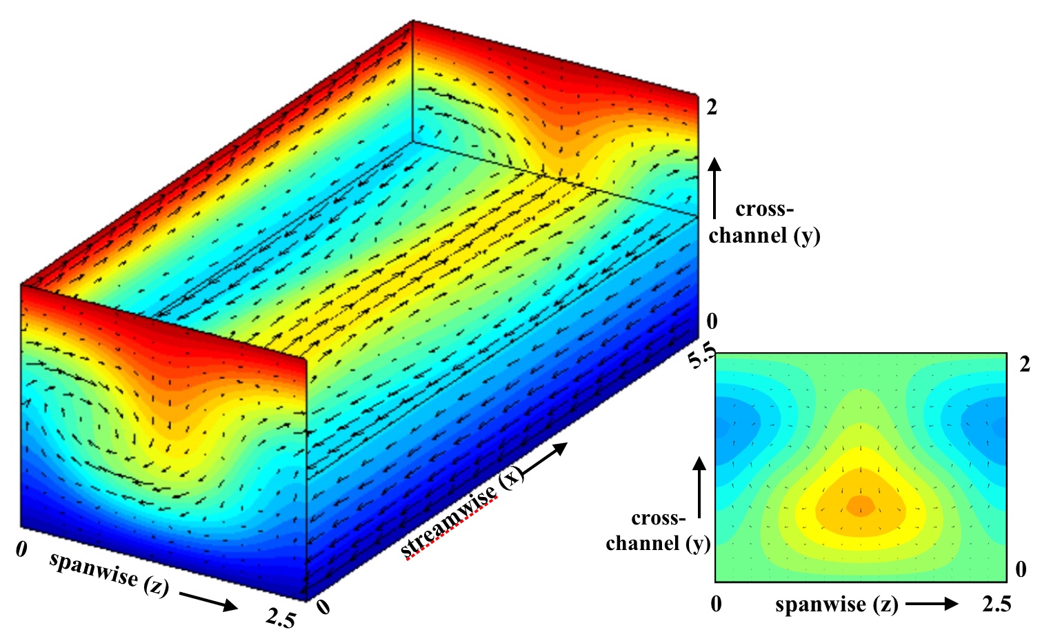
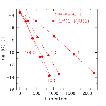
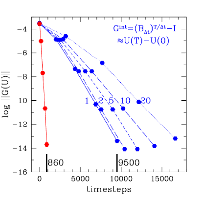
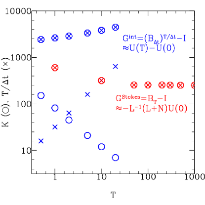
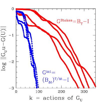
Many steady states of plane Couette flow have been computed using Channelflow; see gibson2009equilibrium . Here, we investigate a branch called EQ1 or NCBW, since it was discovered separately by Nagata Nagata1990three , by Clever & Busse clever1997tertiary and by Waleffe waleffe1998three ; waleffe2003homotopy . It is illustrated in Fig. 1. We begin from a member of EQ1 at $Re=400$ and lower the Reynolds number to $Re=380$. We use a domain of size $2\pi/1.14\times 2\times 2\pi/2.5$ with a numerical resolution of $(M_{x},M_{y},Mz)=(48,35,48)$. At each Newton iteration, the L₂ norm $||G(U)||$ is measured. Each Newton step requires the solution of a linear system, which in turn requires $K\times T/\Delta t$ timesteps. We plot $||G(U)||$ as a function of the timesteps executed. The left portion of Fig. 3 shows that the best performance for the multi-step time-integration-based $G^{\rm int}$ with $\Delta t=0.031\,25$ is achieved for $T\lesssim 1$, while the right portion shows that the best performance for the single-step Stokes-preconditioned $G^{\rm Stokes}$ is achieved for $\Delta t=T\gtrsim 100$. The most striking result of Fig. 3, however, is that the Stokes method takes about 10% of the number of timesteps of the classic integration method.

In order to better understand the performance of these two methods, we recall that the number of timesteps per Newton iteration is the product of $T/\Delta t$ and $K$. For $G^{\rm int}$, $T/\Delta t$ obviously increases with the total integration time $T$, while $K$ decreases with $T$, i.e. $G^{\rm int}$ becomes better conditioned. Figure 3 (left) illustrates this tradeoff. The two effects combine to show a slight increase in number of timesteps with final time $T$. In contrast, for $G^{\rm Stokes}$, the number $K$ of operator actions needed is far higher than is needed for $G^{\rm int}$, but only a single timestep is needed per operator action. This leads to a far lower cost for $G^{\rm Stokes}$ than for $G^{\rm int}$. For $G^{\rm Stokes}$, increasing $T$ makes the preconditioning more effective, leading to a decrease in $K$ and therefore in the number of timesteps taken as shown in the left portions of Fig. 3 and 3. The decrease is monotonic and saturates at around $T=100$. (However, in beaume2017adaptive a local minimum is found, with optimal performance at $T=0.1$.) We emphasize that changing $T$ in $G^{\rm Stokes}$ affects only the rate of convergence. In contrast, the roots themselves of $G^{\rm int}$ necessarily depend somewhat on $\Delta t$ and, to a lesser extent, on $T$ as well. Figure 3 (right) shows the convergence of the solution of the linear systems arising in the successive Newton steps at $Re=500$ for $G^{\rm int}_{T=1}$ and $G^{\rm Stokes}_{T=100}$. Convergence is interrupted by plateaus, whose understanding might lead to better preconditioners. Note that $K$ increases from one Newton step to the next, which is especially noticeable for $G^{\rm Stokes}$.

We have calculated the EQ1 branch from $Re=400$ up to $Re=3000$. The conditioning of both operators worsens: for $Re=2000$, the number of timesteps required by the Stokes preconditioning and the integration methods is about 4000 and 40 000, respectively, while for $Re=3000$, it is about 9000 and 90 000. Thus, the time required increases for both methods, but the ratio between the two methods in terms of number of timesteps remains approximately the same: on the order of 10. For the case of a lid-driven cavity, Brynjell-Rahkola et al. brynjell2017computing show that the number of GMRES iterations required by $G^{\rm Stokes}$ using Nek5000 Nekton is approximately proportional to $Re$, as $Re$ is increased from 100 to 500. It was previously shown tuckerman2015laplacian that the condition number of $G^{\rm Stokes}$ is unaffected by an increase in spatial resolution.

3.4 Computations with Openpipeflow

Figure 4: Traveling wave states N4L (left) and M1L (right), visualized via the deviation of the streamwise velocity from the laminar profile. From Pringle, Duguet and Kerswell pringle2009highly .

Figure 5: Performance of Newton’s method with GMRES in Openpipeflow for single-step Stokes preconditioning method $G^{\rm Stokes}_{T}$ and for multi-step integration method $G^{\rm int}_{T}$ for various values of $T$. The initial condition is the N4L traveling wave state at $Re=2500$ and $Re$ is raised to $Re=2600$. Ordinate shows $\log||G(U)||$ at each Newton iteration, while abscissa shows the number of timesteps taken thus far. Each curve is labelled by its value of $T$. Left: Performance of single-step $G^{\rm Stokes}_{T}\equiv B_{T}-I$. Convergence is fastest when $T$ is highest, achieving approximately asymptotic performance for $T=50$ (solid curve). Right: Performance of multi-step $G^{\rm int}_{T}\equiv(B_{\Delta t})^{T/\Delta t}-I$ with timestep $\Delta t=0.01$. Convergence is fastest when $T$ is lowest, achieving approximately asymptotic performance for $T=1$ (solid curve). Shown for comparison is the convergence curve for $G^{\rm Stokes}$ with $T=50$. Short black lines highlight the difference in speed between the two methods: the classic integration method takes $87\,600$ timesteps, while the Stokes method takes $2520$ timesteps, a ratio of about $35$.

Figure 6: Time taken to compute the highly symmetric M1L state as a function of Reynolds number. Comparison in terms of number of timesteps (left) and CPU time in seconds (right). Computation with single-step $G^{\rm Stokes}_{T}$ uses $T=50$ while computation with multi-step $G^{\rm int}_{T}$ uses $T=5$. The time taken to calculate the traveling waves increases for both the Stokes and the integration method. The ratio of timesteps between the two methods, about 50, changes very little, while the ratio of CPU times decreases from 55 to about 2.

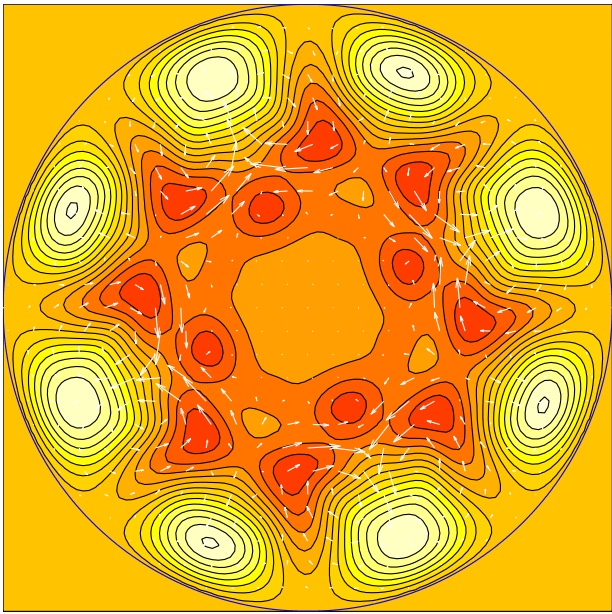
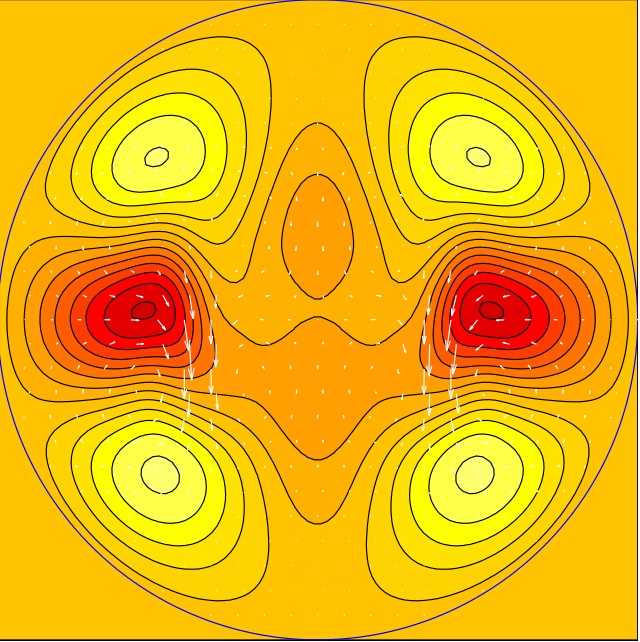
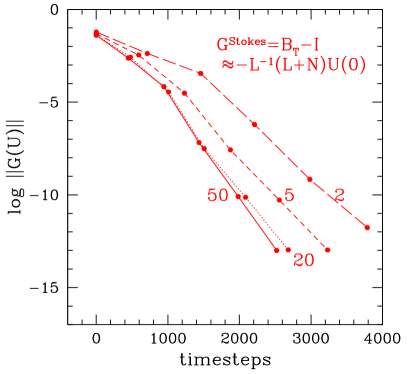
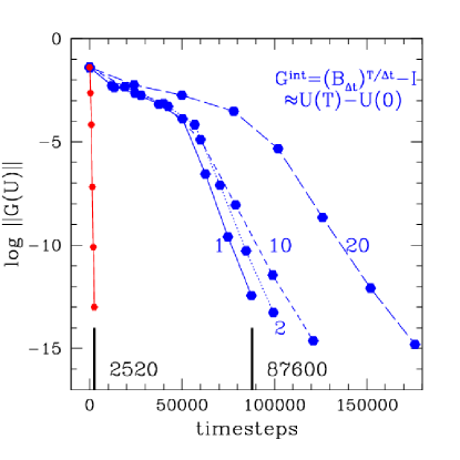
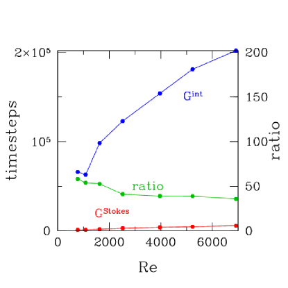
We now turn to calculations carried out using Openpipeflow. Since there is a mean flow along the streamwise direction $x$ of the pipe, bifurcations breaking the $x$ symmetry are always to traveling waves. Visualizations of two such states, namely the N4L and M1L waves computed by Pringle, Duguet and Kerswell pringle2009highly , are given in Fig. 4. Figure 5 presents the convergence of the calculation of N4L at $Re=2600$ with Openpipeflow, starting from the solution at $Re=2500$. (We recall that Reynolds numbers for pipe flow are defined in such a way that that they are 4 to 6 times the equivalent Reynolds numbers for plane Couette flow.) The axial length is $\pi/1.7$ diameters and the resolution is $(M_{r},M_{\theta},M_{z})=(64,36,54)$. Measured in terms of the number of timesteps, the calculation using $G^{\rm Stokes}$ is 35 times faster than that using $G^{\rm int}$. We then calculate states along the highly symmetric M1L branch as a function of Reynolds number. The axial length is $\pi/1.437$ diameters and the resolution is $(M_{r},M_{\theta},M_{z})=(64,48,54)$. The speedup is even more dramatic, reaching a ratio of 50 in terms of timesteps between the Stokes and integration methods. This ratio remains approximately constant as the Reynolds number is increased, as shown in the left portion of Fig. 6.

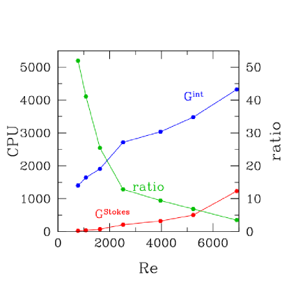
In the right portion of Fig. 6 we contrast the CPU time in seconds required by the two methods on a single processor of a Xeon X5650@2.67GHz. The Stokes method remains much faster than the integration method, but far less than when it is measured in terms of number of timesteps. The reason for this has been alluded to before, in Eq. (28). For sufficiently large $K$ (which occurs at sufficiently high $Re$), the CPU time taken by GMRES to orthogonalize the Krylov vectors to one another, which scales like $K^{2}$, becomes comparable to and even exceeds the CPU time taken by the operator actions.

3.5 Operator Spectra

Figure 7: Spectra in the complex plane of the single-step operators $G^{\rm Stokes}_{0.0001}$ (green), $G^{\rm Stokes}_{0.1}$ (blue), $G^{\rm Stokes}_{100}$ (ochre) and the multi-step operator $G^{\rm int}_{10}$ (magenta) for EQ1 at $Re=500$. (a) The very large negative real eigenvalues of $G^{\rm Stokes}_{0.001}$ near $-360$ are not present in $G^{\rm Stokes}_{0.1}$, for which the dominant eigenvalues have real parts near $-10$ and imaginary parts near $\pm 12$. When $T$ is further increased to 100, most of the real parts cluster within $\pm 0.2$ of $-1$, while the imaginary parts extend to $\pm 35$. (b) Close-up showing the spectra near the point $(-1,0)$. The plotted area is indicated by an overlaid black square in part (a). At this scale, the spectra of the single-step operators are so close as to be indistinguishable, save for a few outliers. Consequently, $G^{\rm Stokes}_{100}$ and $G^{\rm int}_{10}$ have been plotted with larger points for emphasis and only every third point from $G^{\rm Stokes}_{0.0001}$ and $G^{\rm Stokes}_{0.1}$ has been included. The outlying $G^{\rm int}_{10}$ point near $0.6$ is approximately $T=10$ times the leading eigenvalue wang2007lower of $L+N_{U}$. (c) Highly enlarged plot showing the spectrum of $G^{\rm int}_{10}$ only. Most eigenvalues of this well-conditioned multi-step operator cluster tightly around $-1$, since the black circle of radius $8.4\times 10^{-4}$, centered at $(-1,0)$, contains 95% of the spectrum.

Figure 8: Spectra in the complex plane of the single-step operators $G^{\rm Stokes}_{0.0001}$ (green), $G^{\rm Stokes}_{0.1}$ (blue), $G^{\rm Stokes}_{100}$ (ochre) and the multi-step operator $G^{\rm int}_{10}$ (magenta) for EQ1 at $Re=1750$. (a) The most negative eigenvalue of $G^{\rm Stokes}_{0.0001}$ is now near $-105$, while that of $G^{\rm Stokes}_{0.1}$ is near $-10$. An enlargement showing the shape of these two spectra near the origin is included in the top left; its drawing region is indicated by the gray rectangle in the larger plot and its aspect ratio is $1:2$. The real parts of the eigenvalues of $G^{\rm Stokes}_{100}$ continue to cluster around $-1$, but the imaginary parts now extend higher than in the $Re=500$ case, to $\pm 100$. (b) Close-up showing the spectra near the point $(-1,0)$. The plotted area is indicated by an overlaid black square in part (a). The spectra of $G^{\rm int}_{10}$ and $G^{\rm Stokes}_{100}$ have been plotted with larger points to distinguish them from the very dense regions of the $G^{\rm Stokes}_{0.0001}$ and $G^{\rm Stokes}_{0.1}$ spectra, for which we include only every fourth point at this level of enlargement. The outlying $G^{\rm int}_{10}$ point near $0.35$ is $T=10$ times the leading eigenvalue wang2007lower of $L+N_{U}$. (c) Slightly closer enlargement showing only the $G^{\rm int}_{10}$ eigenvalues. The black circle of radius $0.153$, centered at $(-1,0)$, contains $95\%$ of the spectrum. This should be contrasted with the $Re=500$ case in which the eigenvalues are more tightly clustered by roughly two orders of magnitude.

We have seen that the Stokes preconditioning method is much faster than the integration-based method because the time required to act with $G^{\rm Stokes}$ is so much less than that required by $G^{\rm int}$. However, the conditioning of $G^{\rm Stokes}$ is much worse than that of $G^{\rm int}$. We want to understand why this is so and also why the conditioning of both operators worsens as the Reynolds number increases and improves as $T$ increases. To do so, we calculate spectra of branch EQ1 of plane Couette flow using Channelflow. This is done by constructing the full Jacobian matrix by acting with $G^{\rm int}$ or $G^{\rm Stokes}$ on successive basis vectors to form each column. The eigenvalues are determined using Julia, which in turn uses Lapack’s geevx routine.

Figure 7 shows the spectra at $Re=500$ of the Jacobians $G_{U}$ of operators $G^{\rm Stokes}$ and $G^{\rm int}$ for various values of $T$, linearized at EQ1 with spatial resolution $(M_{x},M_{y},M_{z})=(39,29,39)$. Note that these spectra are in general not those of $L+N_{U}$, whose eigenvalues determine the stability of the steady states via the sign of their real parts. Instead, the $G$’s are operators whose roots are the same as those of $L+N$ but whose spectra may be quite different. Newton’s method finds the roots of the $G$ operators independent of their stability. (We do not recommend any of these operators as a means of determining eigenvalues of $L+N_{U}$. Other, more precise and more economical methods are given in wang2007lower via exact diagonalization of the Jacobian, in sanchez2004newton ; viswanath2007recurrent ; gibson2008visualizing via more accurate use of $G^{\rm int}$, and in barkley1997stokes ; IMA ; huepe2003stability ; tuckerman2015laplacian via the inverse Arnoldi method with Stokes preconditioning.) Our interest is instead in the distribution of the eigenvalues of the Jacobians $G_{U}$, which determines the rate of convergence of GMRES in solving the linear systems (17). Broadly speaking, a tightly clustered spectrum leads to fast convergence, a highly dispersed spectrum to slow convergence. In order to compare the spectra of $G^{\rm Stokes}_{T}$ at different values of $T$, we have followed beaume2017adaptive and rescaled the eigenvalues $\lambda^{\text{Stokes}}$ via:

$$\lambda^{\text{Stokes}}\mapsto\frac{1+T}{T}\lambda^{\text{Stokes}}.$$ (29)

(Note that scaling does not change the condition number of an operator.) The scaling factor is $1/T$ in the limit of small $T$ and $1$ for large $T$. It is designed to remove the $\Delta t$ ($=T$) dependence from the limiting behaviors of the Stokes operator given in (10) and (11) and thereby facilitate the visual comparison of the spectra at different values of $T$ at approximately the same scales. Using (29), the eigenvalues tend to those of $L+N_{U}$ as $T\rightarrow 0$ and to those of $-L^{-1}(L+N_{U})$ as $T\rightarrow\infty$. The green points show the spectrum of $G^{\rm Stokes}$ for $T=10^{-4}$, a value small enough for $G^{\rm Stokes}$ to resemble $L+N_{U}$. The large negative eigenvalues of the Laplacian (or rather its vector analogue, the Stokes operator) are prominent outlying features. Here, the spectrum extends to $-360$, but these eigenvalues depend on the spatial resolution, becoming more negative as the resolution is increased. It is these eigenvalues that are responsible for the poor conditioning of $L+N_{U}$, or equivalently, the stiffness of the Navier-Stokes equations. As $T=\Delta t$ is increased to $10^{-1}$ (blue points), the eigenvalues retract towards zero and are contained approximately within the convex hull of the points $(-11,0)$, $(-1,\pm 13\>i)$, and the origin. When $T=\Delta t$ is increased to 100 (ochre points), in the asymptotic regime used in steady-state solving, the spectrum lies very close to the line segment between $(-1,-30i)$ and $(-1,30i)$; over 95% of the eigenvalues possess real part within $\pm 0.2$ of $-1$. The real range has decreased drastically, but the imaginary range has increased. Brynjell-Rahkola et al. brynjell2017computing also show that the eigenvalues of $G^{\rm Stokes}_{T}$ converge towards a curve as $T$ is increased for the model problem of a Ginzburg-Landau equation.

The eigenvalues of the multi-step operator $G^{\rm int}_{T=10}$ with $\Delta t=0.031\,25$ are shown as magenta points. The Jacobian of $(B_{\Delta t})^{T/\Delta t}$ should approach $\exp(T(L+N_{U}))$ as $\Delta t\rightarrow 0$. This leads to the following limits for the eigenvalues $\lambda^{\text{int}}$ of $G^{\rm int}$, in terms of the eigenvalues $\lambda$ of $L+N_{U}$:

$$\lambda^{\text{int}}\approx\exp(\lambda T)-1\approx\left\{\begin{array}[]{l}\lambda T\\ -1\end{array}\right\}\mbox{~{}~{}for~{}~{}}\left\{\begin{array}[]{l}|\lambda T|\ll 1\\ |\lambda T|\gg 1,\mbox{~{}~{}with~{}~{}}\lambda<0\end{array}\right\}$$ (30)

which explains why the Jacobian of $G^{\rm int}$ typically enjoys superior conditioning properties. This can be seen by examining Fig. 7, parts (b) and (c), which indeed contain values tightly clustered around $-1$ as well as a positive eigenvalue near 0.6, which is approximately $T=10$ times the known wang2007lower leading eigenvalue 0.06 of EQ1 at $Re=500$. In contrast, while the ochre points of the $G^{\rm Stokes}_{100}$ spectrum cluster in the real direction, their imaginary parts are spread out and the operator is therefore more poorly conditioned.

Comparable spectra for $Re=1750$ are shown in Fig. 8. These differ quantitatively but not qualitatively from those in Fig. 7 for $Re=500$. We use these differences to test the representation of the spectrum of $L+N_{U}$ by that of a 1D model for an advection-diffusion equation with analytical eigenvalues:

$$\lambda_{k}^{\rm model}=-k^{2}/Re\pm ikU$$ (31)

where $k$ represents a wavenumber associated with eigenmodes $e^{ikx}$, whose images under the diffusion and linearized advection operators, respectively, lead to the real and imaginary parts of $\lambda_{k}^{\rm model}$. (Although $k$ has been used previously to designate a member of the sequence of Krylov vectors, we use it again here because it is the universal notation for a wavenumber.) In the following, we assess this model using quantitative comparisons with the eigenvalues for $G^{\rm Stokes}_{T}$, rescaled according to Eq. (29), and $G^{\rm int}_{10}$. We first consider the most negative real eigenvalue of $L+N_{U}$, which is predicted by (31) to be proportional to $1/Re$. The most negative eigenvalue among the green points of $G^{\rm Stokes}_{0.0001}$ in Fig. 8(a) is $-105$, compared to $-360$ for $Re=500$. The ratio of eigenvalues $360/105$ is $3.4$, almost exactly the inverse of the ratio of Reynolds numbers $1750/500=3.5$, as predicted by (31). Our second test concerns the imaginary part of the spectrum of $G^{\rm Stokes}_{T}$. For $T$ large, the model spectrum (31) is transformed under Stokes preconditioning to the vertical line

$$\lambda_{k}^{\rm Stokes}\approx\frac{\lambda_{k}^{\rm model}}{k^{2}/Re}=-1\pm iURe/k,$$ (32)

which resembles the spectrum of $G^{\rm Stokes}_{100}$ aligned along the imaginary axis. To verify the scaling, note that for $Re=1750$, the largest imaginary part among the ochre points of $G^{\rm Stokes}_{100}$ is $\pm 100$, compared with $\pm 35$ for $Re=500$. The ratio between these values is 2.9, close to the ratio between the Reynolds numbers.

For our third test, we use (31) to estimate the radius $r$ of the circle surrounding $(-1,0)$ which contains 95% of the eigenvalues of $G^{\rm int}$. Using the limits in (30), we assume that these eigenvalues correspond to those of (31) with $k>k_{\ast}$. We have

$$\left|\lambda_{k}^{\text{int}}+1\right| \lesssim e^{-Tk_{\ast}^{2}/Re}=r$$ (33)

and therefore

$$Tk_{\ast}^{2}/Re =\ln(1/r),$$ (34)

yielding another expression for the ratio between Reynolds numbers $$Re_{1} Re_{2}$$ and :

$$\frac{Re_{2}}{Re_{1}} =\frac{\ln(1/r_{1})}{\ln(1/r_{2})}.$$ (35)

The radii measured for $$Re_{1}=500 Re_{2}=1750 r_{1}=0.000\,84 r_{2}=0.153$$ and are and , respectively, leading to

$$\frac{\ln(1/0.000\,84)}{\ln(1/0.153)} =\frac{7.08}{1.877}=3.77,$$ (36)

which is again very close to $1750/500=3.5$.

When $T$ is changed and $Re$ kept constant, (34) implies that the left-hand-side of (35) should be replaced by $T_{1}/T_{2}$. We have verified this for $Re=500$ by computing the radius $0.049$ containing 95% of the eigenvalues for $G^{\rm int}_{T=1}$. Comparing this to the radius corresponding to $G^{\rm int}_{T=10}$ yields

$$\frac{\ln(1/0.00084)}{\ln(1/0.049)}=10.003$$ (37)

very close to the ratio of the $T$ values. To preserve the conditioning of $G^{\rm int}$ as $Re$ is increased, the ratio $T/Re$ should be kept constant. Since the time taken to act with $G^{\rm int}$ is proportional to $T/\Delta t$, we arrive at the useful result that the CPU time taken by $G^{\rm int}$ to calculate steady states or traveling waves is, in the absence of changes in the spatial or temporal resolution, proportional to the Reynolds number. The number of timesteps taken by $G^{\rm Stokes}$ is also approximately proportional to $Re$, as shown in Fig. 6(left) and in brynjell2017computing .

The true spectrum of $L+N_{U}$ is certainly more complicated than (31). The green dots in Fig. 7 and 8 show many features not present in (31) and indeed, the eigenvalues of $L$ and $N_{U}$ are not as simple as $-k^{2}/Re$ and $\pm ikU$. Note, however, that the only features of (31) that we have used are shared by the more general model

$${\lambda_{k}^{\rm model}}^{~{}\prime}=-f(k)/Re\pm ig(k)$$ (38)

in which $k$ serves merely as an index enumerating the eigenvalues. The astonishing accuracy of the predictions of this model leads us to believe that it provides a good representation of the basic shape of the actual spectra and operators. Moreover, it provides a simple explanation of the dependence of the spectra on $Re$ and $T$ and by extension, the conditioning properties of the operators.

3.6 Challenges

We close by mentioning the limitations and applicability of the Stokes preconditioning method. First, the single-step Stokes operator can be used only for computing steady states and traveling waves and not for calculating general periodic orbits or more complex dynamical states. It seems unlikely that any generalization would be possible, since even describing or defining these objects necessarily requires multiple time steps. However, Stokes preconditioning can be used to rapidly compute leading eigenvalues barkley1997stokes ; IMA ; huepe2003stability ; tuckerman2015laplacian and optimal forcing brynjell2017computing via the inverse power or Arnoldi method. Second, Stokes preconditioning is based on the utility and speed of inverting elliptic (Laplacian, Stokes, or Helmholtz) operators. Concerning utility, Stokes preconditioning is an effective preconditioner for the Jacobian $L+N_{U}$ under precisely the same conditions that implicit timestepping of the diffusive/viscous operator $L$ is effective. Concerning speed, the most favorable conditions occur when the elliptic operators are inverted directly rather than iteratively, which is easy in a tensor-product domain tuckerman1989steady ; lynch1964direct ; haidvogel1979accurate ; vitoshkin2013direct . Codes such as Nek5000 Nekton , which use spectral elements to represent flexible user-defined geometries, typically do not do so. Instead, these codes use iterative methods whose convergence relies on the Helmholtz operators $I-\Delta tL$ being close to the identity, which is not the case when $\Delta t$ is taken large. Similarly, codes sometimes impose constraints, notably incompressibiity, to a power of $\Delta t$ rather to machine accuracy; this too is not compatible with large $\Delta t$. However, based on the experience of previous researchers using spectral element methods we believe that these objections can be overcome.

We have seen that Stokes preconditioning is extremely economical at the lower Reynolds number ranges of our investigation, achieving a 50-fold economy in CPU time. This factor, however, decreases as the Reynolds number increases, and we have been able to understand the reason for this. As $Re$ increases, the Jacobian $L+N_{U}$ deviates increasingly from $L$, preconditioning by $L^{-1}$ becomes less effective, and so the number $K$ of iterations necessary to solve each linear system increases. The consequences of this are particularly severe when GMRES is used, since part of its algorithm requires a time which is quadratic in $K$. We can propose several remedies for this, in increasing order of difficulty and effectiveness. First, $K$ may be reduced by relaxing the convergence criterion for solving the linear equation (17). This has the counterbalancing effect of increasing the number of Newton steps required, but some improvement is possible. A more promising approach is to use a different method for solving the linear systems. Conjugate-gradient-type methods other than GMRES, notably BiCGSTAB, do not retain all $K$ Krylov vectors throughout the calculation. Hence, they do not store $K$ velocity fields and no portion of their operation count scales like $K^{2}$. Although BiCGSTAB has been widely used in the applications of Stokes preconditioning detailed in the introduction, we have not succeeded in doing so in Channelflow or in Openpipeflow. The reason for this is probably given in Figs. 7 and 8: as the Reynolds number is increased, the eigenvalues associated with $G^{\rm Stokes}$ acquire large imaginary parts and BiCGSTAB is known to converge badly in this case gutknecht1993variants ; sleijpen1993bicgstab . Related methods, such as BiCGSTAB($\ell$) and IDR sonneveld2008idr that act better with such matrices have been proposed. The most promising idea, inspired by Figs. 7 and 8 and the model (38) is to incorporate linear portions of $N$ into $L$, in particular the linearization around the laminar flow

$$\left(\mathbf{U}_{\rm lam}\cdot\nabla\right)\mathbf{u}+\left(\mathbf{u}\cdot\nabla\right)\mathbf{U}_{\rm lam}$$ (39)

so as to include a large part of the advective term in the preconditioning.

Appendix

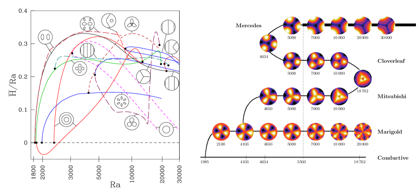
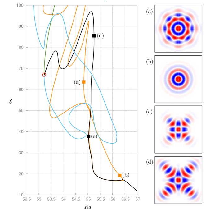
This Appendix presents samples in Figs. 10, 10, 11 and 12 of previous computations carried out by Stokes preconditioning.

Figure 9: Rayleigh-Bénard convection in a cylinder of aspect ratio with radius / height $=2$, $Pr=6.7$ and insulating lateral boundaries. Left: Bifurcation diagram shows 17 branches of steady states, with azimuthal symmetries $m=2$ (pizza, four-roll), $m=0$ (two-tori, torus), $m=3$ (marigold, Mitsubishi, cloverleaf, Mercedes), $m=1$ (dipole, three-roll, tiger, asymmetric three-roll). Right: Partial schematic diagram showing branches with $m=3$ symmetry. Transition from conductive state to marigold and then Mitsubishi branches occur via circle and ordinary pitchfork bifurcations, respectively, and to cloverleaf and Mercedes branches via two successive saddle-node bifurcations. The only stable states are on a portion of the Mercedes branch, shown by the thick curve. The results are from a pseudospectral simulation with $(M_{r},M_{\theta},M_{z})=(60,130,30)$. From Borońska & Tuckerman boronska2010extreme .

Figure 10: Binary fluid convection in a domain with aspect ratio width / height $=14$, Neumann boundary conditions, Prandtl and Lewis numbers $Pr=7$, $Le=0.01$ and separation ratio $S=-0.1$. Left: Partial bifurcation diagram showing two-pulse point-symmetric states based on 15 rolls. Right: Temperature and concentration fields for the three solutions indicated as dots on the bifurcation diagram. From Mercader, Batiste, Alonso & Knobloch mercader2011convectons .

Figure 11: Three-dimensional binary fluid convection in a porous medium of size $6\times 6\times 1$. Left: bifurcation diagram. Right: vertical velocity at mid-layer. The transition from a four-armed structure with arms oriented along the diagonals (panels (c) and (d), black curve) to an eight-armed structure with arms oriented along both the diagonals and the principal axes of the domain (panel (a), orange curve) via a target pattern (panel (b)). Simulations use a spectral element method with 6 elements in the quarter domain, each with $(23,23,17)$ points. From LoJacono, Bergeon & Knobloch jacono2017complex .

Figure 12: Steady states of a streamwise-independent reduced model for plane Couette flow. Bifurcation diagram on left. Representative states from lower (middle) and upper (right) branches at $Re\approx 1000$. Colored contours show the streamfunction of streamwise rolls, while the black curves show contours of the streamwise velocity. From Beaume, Chini, Julien & Knobloch beaume2015reduced ; beaume2017adaptive .

References

- (1) Laurette S Tuckerman. Steady-state solving via Stokes preconditioning; recursion relations for elliptic operators. In R.G. Voigt D.L. Dwoyer, M.Y. Hussaini, editor, 11th Int. Conf. Num. Meth. Fluid Dyn., pages 573–577. Springer, 1989.
- (2) Chowdhury K Mamun and Laurette S Tuckerman. Asymmetry and Hopf bifurcation in spherical Couette flow. Phys. Fluids, 7:80–91, 1995.
- (3) Shihe Xin, Patrick Le Quéré, and Olivier Daube. Natural convection in a differentially heated horizontal cylinder: Effects of Prandtl number on flow structure and instability. Phys. Fluids, 9:1014–1033, 1997.
- (4) Shihe Xin and Patrick Le Quéré. An extended Chebyshev pseudo-spectral benchmark for the 8: 1 differentially heated cavity. Int. J. Numer. Meth. Fluids, 40:981–998, 2002.
- (5) Shihe Xin and Patrick Le Quéré. Stability of two-dimensional (2D) natural convection flows in air-filled differentially heated cavities: 2D/3D disturbances. Fluid Dyn. Res., 44:031419, 2012.
- (6) Eric Chénier, Claudine Delcarte, and Gérard Labrosse. Stability of the axisymmetric buoyant-capillary flows in a laterally heated liquid bridge. Phys. Fluids, 11:527–541, 1999.
- (7) Isabel Mercader, Oriol Batiste, Laureano Ramírez-Piscina, Xavier Ruiz, S Rüdiger, and J Casademunt. Bifurcations and chaos in single-roll natural convection with low Prandtl number. Phys. Fluids, 17:104108, 2005.
- (8) Daniel Henry and Hamda BenHadid. Multiple flow transitions in a box heated from the side in low-Prandtl-number fluids. Phys. Rev. E, 76:016314, 2007.
- (9) Walid Dridi, Daniel Henry, and H Ben Hadid. Influence of acoustic streaming on the stability of a laterally heated three-dimensional cavity. Phys. Rev. E, 77:046311, 2008.
- (10) Juan F Torres, Daniel Henry, Atsuki Komiya, Shigenao Maruyama, and H Ben Hadid. Three-dimensional continuation study of convection in a tilted rectangular enclosure. Phys. Rev. E, 88:043015, 2013.
- (11) Juan F Torres, Daniel Henry, Atsuki Komiya, and Shigenao Maruyama. Bifurcation analysis of steady natural convection in a tilted cubical cavity with adiabatic sidewalls. J. Fluid Mech., 756:650–688, 2014.
- (12) Juan F Torres, Daniel Henry, Atsuki Komiya, and Shigenao Maruyama. Transition from multiplicity to singularity of steady natural convection in a tilted cubical enclosure. Phys. Rev. E, 92:023031, 2015.
- (13) Ridha Touihri, Hamda BenHadid, and Daniel Henry. On the onset of convective instabilities in cylindrical cavities heated from below. I. Pure thermal case. Phys. Fluids, 11:2078–2088, 1999.
- (14) Ridha Touihri, Anas El Gallaf, Daniel Henry, and Hamda BenHadid. Instabilities in a cylindrical cavity heated from below with a free surface. I. Effect of Biot and Marangoni numbers. Phys. Rev. E, 84:056302, 2011.
- (15) Pauline Assemat, Alain Bergeon, and Edgar Knobloch. Nonlinear Marangoni convection in circular and elliptical cylinders. Phys. Fluids, 19:104101, 2007.
- (16) Francisco Marques, Isabel Mercader, Oriol Batiste, and Juan M Lopez. Centrifugal effects in rotating convection: axisymmetric states and three-dimensional instabilities. J. Fluid Mech., 580:303–318, 2007.
- (17) Katarzyna Borońska and Laurette S Tuckerman. Extreme multiplicity in cylindrical Rayleigh-Bénard convection. II. Bifurcation diagram and symmetry classification. Phys. Rev. E, 81:036321, 2010.
- (18) Isabel Mercader, Odalys Sánchez, and Oriol Batiste. Secondary flows in a laterally heated horizontal cylinder. Phys. Fluids, 26:014104, 2014.
- (19) Odalys Sánchez, Isabel Mercader, Oriol Batiste, and Arantxa Alonso. Natural convection in a horizontal cylinder with axial rotation. Phys. Rev. E, 93:063113, 2016.
- (20) Kay Bergemann, Fred Feudel, and Laurette S Tuckerman. Geoflow: On symmetry-breaking bifurcations of heated spherical shell convection. In J. Phys. Conf. Ser., volume 137, page 012027. IOP Publishing, 2008.
- (21) Fred Feudel, Kay Bergemann, Laurette S Tuckerman, Christoph Egbers, Birgit Futterer, Marcus Gellert, and Rainer Hollerbach. Convection patterns in a spherical fluid shell. Phys. Rev. E, 83:046304, 2011.
- (22) Fred Feudel, Norbert Seehafer, Laurette S Tuckerman, and Marcus Gellert. Multistability in rotating spherical shell convection. Phys. Rev. E, 87:023021, 2013.
- (23) Fred Feudel, Laurette S Tuckerman, Marcus Gellert, and Norbert Seehafer. Bifurcations of rotating waves in rotating spherical shell convection. Phys. Rev. E, 92:053015, 2015.
- (24) F Feudel, Laurette S Tuckerman, M Zaks, and R Hollerbach. Hysteresis of dynamos in rotating spherical shell convection. Phys. Rev. F, 2:053902, 2017.
- (25) Olivier Daube and Patrick Le Quéré. Numerical investigation of the first bifurcation for the flow in a rotor–stator cavity of radial aspect ratio 10. Computers & fluids, 31:481–494, 2002.
- (26) Caroline Nore, Laurette S Tuckerman, Olivier Daube, and Shihe Xin. The 1 [ratio] 2 mode interaction in exactly counter-rotating von kármán swirling flow. J. Fluid Mech., 477:51–88, 2003.
- (27) Caroline Nore, Michaël Tartar, Olivier Daube, and Laurette S Tuckerman. Survey of instability thresholds of flow between exactly counter-rotating disks. J. Fluid Mech., 511:45–65, 2004.
- (28) Cristian Huepe, Stéphane Metens, Guy Dewel, Pierre Borckmans, and Marc-Etienne Brachet. Decay rates in attractive Bose-Einstein condensates. Phys. Rev. Lett., 82:1616, 1999.
- (29) Malek Abid, Cristian Huepe, Stéphane Metens, Caroline Nore, Chi Tuong Pham, Laurette S Tuckerman, and Marc Etienne Brachet. Gross–Pitaevskii dynamics of Bose–Einstein condensates and superfluid turbulence. Fluid Dyn. Res., 33:509–544, 2003.
- (30) Shihe Xin, Patrick Le Quéré, and Laurette S Tuckerman. Bifurcation analysis of double-diffusive convection with opposing horizontal thermal and solutal gradients. Phys. Fluids, 10:850–858, 1998.
- (31) Alain Bergeon, Daniel Henry, Hamda Benhadid, and Laurette S Tuckerman. Marangoni convection in binary mixtures with soret effect. J. Fluid Mech., 375:143–177, 1998.
- (32) Alain Bergeon, K Ghorayeb, and A Mojtabi. Double diffusive instability in an inclined cavity. Phys. Fluids, 11:549–559, 1999.
- (33) Gérald Bardan, Alain Bergeon, Edgar Knobloch, and Abdelkader Mojtabi. Nonlinear doubly diffusive convection in vertical enclosures. Physica D, 138:91–113, 2000.
- (34) Alain Bergeon and Edgar Knobloch. Natural doubly diffusive convection in three-dimensional enclosures. Phys. Fluids, 14:3233–3250, 2002.
- (35) Alain Bergeon, R Mollaret, and D Henry. Soret effect and slow mass diffusion as a catalyst for overstability in Marangoni-Bénard flows. Heat Mass Transf., 40:105–114, 2003.
- (36) Esteban Meca, Isabel Mercader, Oriol Batiste, and Laureano Ramírez-Piscina. Blue sky catastrophe in double-diffusive convection. Phys. Rev. Lett., 92:234501, 2004.
- (37) Esteban Meca, Isabel Mercader, Oriol Batiste, and Laureano Ramírez-Piscina. Complex dynamics in double-diffusive convection. Theoret. Comput. Fluid Dyn., 18:231–238, 2004.
- (38) Isabel Mercader, Arantxa Alonso, and Oriol Batiste. Numerical analysis of the Eckhaus instability in travelling-wave convection in binary mixtures. Eur. Phys. J. E, 15:311–318, 2004.
- (39) Oriol Batiste, Arantxa Alonso, and Isabel Mercader. Hydrodynamic stability of binary mixtures in Bénard and thermogravitational cells. Journal of Non-Equilibrium Thermodynamics, 29:359–375, 2004.
- (40) Arantxa Alonso, Oriol Batiste, and Isabel Mercader. Numerical analysis of binary fluid convection in extended systems. In J. Phys. Conf. Ser., volume 14, page 180. IOP Publishing, 2005.
- (41) Arantxa Alonso, Oriol Batiste, Alvaro Meseguer, and Isabel Mercader. Complex dynamical states in binary mixture convection with weak negative soret coupling. Phys. Rev. E, 75:026310, 2007.
- (42) John Burke and Edgar Knobloch. Localized states in the generalized Swift-Hohenberg equation. Phys. Rev. E, 73:056211, 2006.
- (43) Alan R Champneys. Homoclinic orbits in reversible systems and their applications in mechanics, fluids and optics. Physica D, 112:158–186, 1998.
- (44) Pierre Coullet, C Riera, and Charles Tresser. Stable static localized structures in one dimension. Phys. Rev. Lett., 84:3069, 2000.
- (45) Stephan Fauve and Olivier Thual. Solitary waves generated by subcritical instabilities in dissipative systems. Phys. Rev. Lett., 64:282, 1990.
- (46) Yves Pomeau. Front motion, metastability and subcritical bifurcations in hydrodynamics. Physica D, 23:3–11, 1986.
- (47) M’F Hilali, Stéphane Métens, Pierre Borckmans, and Guy Dewel. Pattern selection in the generalized Swift-Hohenberg model. Phys. Rev. E, 51:2046, 1995.
- (48) Oriol Batiste, Edgar Knobloch, Arantxa Alonso, and Isabel Mercader. Spatially localized binary-fluid convection. J. Fluid Mech., 560:149–158, 2006.
- (49) Arantxa Alonso, Oriol Batiste, and Isabel Mercader. Numerical simulations of binary fluid convection in large aspect ratio annular containers. Eur. Phys. J. Spec. Top., 146:261–277, 2007.
- (50) Alain Bergeon and Edgar Knobloch. Spatially localized states in natural doubly diffusive convection. Phys. Fluids, 20:034102, 2008.
- (51) Alain Bergeon and Edgar Knobloch. Periodic and localized states in natural doubly diffusive convection. Physica D, 237:1139–1150, 2008.
- (52) Pauline Assemat, Alain Bergeon, and Edgar Knobloch. Spatially localized states in Marangoni convection in binary mixtures. Fluid Dyn. Res., 40:852–876, 2008.
- (53) David LoJacono, Alain Bergeon, and Edgar Knobloch. Spatially localized binary fluid convection in a porous medium. Phys. Fluids, 22:909, 2010.
- (54) Cédric Beaume, Alain Bergeon, and Edgar Knobloch. Homoclinic snaking of localized states in doubly diffusive convection. Phys. Fluids, 23:094102, 2011.
- (55) Isabel Mercader, Oriol Batiste, Arantxa Alonso, and Edgar Knobloch. Convectons, anticonvectons and multiconvectons in binary fluid convection. J. Fluid Mech., 667:586–606, 2011.
- (56) Cédric Beaume, Alain Bergeon, Hsien-Ching Kao, and Edgar Knobloch. Convectons in a rotating fluid layer. J. Fluid Mech., 717:417–448, 2013.
- (57) Cédric Beaume, Edgar Knobloch, and Alain Bergeon. Nonsnaking doubly diffusive convectons and the twist instability. Phys. Fluids, 25:114102, 2013.
- (58) Isabel Mercader, Oriol Batiste, Arantxa Alonso, and Edgar Knobloch. Travelling convectons in binary fluid convection. J. Fluid Mech., 722:240–266, 2013.
- (59) David LoJacono, Alain Bergeon, and Edgar Knobloch. Spatially localized radiating diffusion flames. Combustion and Flame, 176:117–124, 2017.
- (60) David LoJacono, Alain Bergeon, and Edgar Knobloch. Localized traveling pulses in natural doubly diffusive convection. Phys. Rev. F, 2:093501, 2017.
- (61) David LoJacono, Alain Bergeon, and Edgar Knobloch. Complex convective structures in three-dimensional binary fluid convection in a porous medium. Fluid Dyn. Res., 49:061402, 2017.
- (62) Masato Nagata. Three-dimensional finite-amplitude solutions in plane Couette flow: bifurcation from infinity. J. Fluid Mech., 217:519–527, 1990.
- (63) Fabian Waleffe. Three-dimensional coherent states in plane shear flows. Phys. Rev. Lett., 81:4140, 1998.
- (64) Fabian Waleffe. Exact coherent structures in channel flow. J. Fluid Mech., 435:93–102, 2001.
- (65) Fabian Waleffe. Homotopy of exact coherent structures in plane shear flows. Phys. Fluids, 15:1517–1534, 2003.
- (66) RM Clever and Fritz H Busse. Tertiary and quaternary solutions for plane Couette flow. J. Fluid Mech., 344:137–153, 1997.
- (67) Masato Nagata. Three-dimensional traveling-wave solutions in plane Couette flow. Phys. Rev. E, 55:2023, 1997.
- (68) Holger Faisst and Bruno Eckhardt. Transition from the Couette-Taylor system to the plane Couette system. Phys. Rev. E, 61:7227, 2000.
- (69) Armin Schmiegel. Transition to turbulence in linearly stable shear flows. PhD thesis, Philipps-Universität Marburg, 1999. http://archiv.ub.uni-marburg.de/diss/z2000/0062/.
- (70) Holger Faisst and Bruno Eckhardt. Traveling waves in pipe flow. Phys. Rev. Lett., 91:224502, 2003.
- (71) Hakan Wedin and Rich R Kerswell. Exact coherent structures in pipe flow: travelling wave solutions. J. Fluid Mech., 508:333–371, 2004.
- (72) Predrag Cvitanović. Periodic orbits as the skeleton of classical and quantum chaos. Physica D, 51:138–151, 1991.
- (73) Predrag Cvitanovic and Bruno Eckhardt. Periodic orbit expansions for classical smooth flows. Journal of Physics A: Mathematical and General, 24:L237, 1991.
- (74) Genta Kawahara and Shigeo Kida. Periodic motion embedded in plane Couette turbulence: regeneration cycle and burst. J. Fluid Mech., 449:291–300, 2001.
- (75) Genta Kawahara, Markus Uhlmann, and Lennaert Van Veen. The significance of simple invariant solutions in turbulent flows. Annu. Rev. Fluid Mech., 44:203–225, 2012.
- (76) John E Dennis Jr and Robert B Schnabel. Numerical methods for unconstrained optimization and nonlinear equations, volume 16. SIAM, 1996.
- (77) Dana A Knoll and David E Keyes. Jacobian-free Newton-Krylov methods: a survey of approaches and applications. J. Comput. Phys., 193:357–397, 2004.
- (78) Juan Sánchez, Marta Net, Bosco Garcıa-Archilla, and Carles Simó. Newton-Krylov continuation of periodic orbits for Navier–Stokes flows. J. Comput. Phys., 201:13–33, 2004.
- (79) Divakar Viswanath. Recurrent motions within plane Couette turbulence. J. Fluid Mech., 580:339–358, 2007.
- (80) Lennaert Van Veen, Genta Kawahara, and Matsumura Atsushi. On matrix-free computation of 2D unstable manifolds. SIAM J. Sci. Comput., 33:25–44, 2011.
- (81) Chris CT Pringle and Rich R Kerswell. Asymmetric, helical, and mirror-symmetric traveling waves in pipe flow. Phys. Rev. Lett., 99:074502, 2007.
- (82) Rich R Kerswell and Owen R Tutty. Recurrence of travelling waves in transitional pipe flow. J. Fluid Mech., 584:69–102, 2007.
- (83) Yohann Duguet, Ashley P Willis, and Rich R Kerswell. Transition in pipe flow: the saddle structure on the boundary of turbulence. J. Fluid Mech., 613:255–274, 2008.
- (84) Yohann Duguet, Chris CT Pringle, and Rich R Kerswell. Relative periodic orbits in transitional pipe flow. Phys. Fluids, 20:114102, 2008.
- (85) John F Gibson, Jonathan Halcrow, and Predrag Cvitanović. Visualizing the geometry of state space in plane Couette flow. J. Fluid Mech., 611:107–130, 2008.
- (86) John F Gibson, Jonathan Halcrow, and Predrag Cvitanović. Equilibrium and travelling-wave solutions of plane Couette flow. J. Fluid Mech., 638:243–266, 2009.
- (87) Chris CT Pringle, Yohann Duguet, and Rich R Kerswell. Highly symmetric travelling waves in pipe flow. Phil. Trans. R. Soc. Lond. A, 367:457–472, 2009.
- (88) John F. Gibson. Channelflow: A spectral Navier-Stokes simulator in C++. Technical report, U. New Hampshire, 2014. Channelflow.org.
- (89) Ashley P Willis. The openpipeflow Navier–Stokes solver. SoftwareX, 6:124–127, 2017.
- (90) Tobias M Schneider, John F Gibson, and John Burke. Snakes and ladders: localized solutions of plane Couette flow. Phys. Rev. Lett., 104:104501, 2010.
- (91) Marc Avila, Fernando Mellibovsky, Nicolas Roland, and Bjoern Hof. Streamwise-localized solutions at the onset of turbulence in pipe flow. Phys. Rev. Lett., 110:224502, 2013.
- (92) John F Gibson and Evan Brand. Spanwise-localized solutions of planar shear flows. J. Fluid Mech., 745:25–61, 2014.
- (93) Evan Brand and John F Gibson. A doubly localized equilibrium solution of plane Couette flow. J. Fluid Mech., 750, 2014.
- (94) Bruno Eckhardt. Doubly localized states in plane Couette flow. J. Fluid Mech., 758:1–4, 2014.
- (95) Matthew Chantry, Ashley P Willis, and Rich R Kerswell. Genesis of streamwise-localized solutions from globally periodic traveling waves in pipe flow. Phys. Rev. Lett., 112:164501, 2014.
- (96) F Mellibovsky and Bruno Eckhardt. Takens–Bogdanov bifurcation of travelling-wave solutions in pipe flow. Journal of fluid mechanics, 670:96–129, 2011.
- (97) Cédric Beaume, Gregory P Chini, Keith Julien, and Edgar Knobloch. Reduced description of exact coherent states in parallel shear flows. Phys. Rev. E, 91:043010, 2015.
- (98) Cédric Beaume, Edgar Knobloch, Gregory P Chini, and Keith Julien. Modulated patterns in a reduced model of a transitional shear flow. Physica Scripta, 91:024003, 2016.
- (99) Jue Wang, John Gibson, and Fabian Waleffe. Lower branch coherent states in shear flows: transition and control. Phys. Rev. Lett., 98:204501, 2007.
- (100) Hugh M Blackburn, Philip Hall, and Sherwin J Sherwin. Lower branch equilibria in Couette flow: the emergence of canonical states for arbitrary shear flows. J. Fluid Mech., 726, 2013.
- (101) Kengo Deguchi and Philip Hall. The high-Reynolds-number asymptotic development of nonlinear equilibrium states in plane Couette flow. J. Fluid Mech., 750:99–112, 2014.
- (102) Youcef Saad and Martin H Schultz. GMRES: A generalized minimal residual algorithm for solving nonsymmetric linear systems. SIAM J. Sci. Comput., 7:856–869, 1986.
- (103) Henk A Van der Vorst. Bi-CGSTAB: A fast and smoothly converging variant of bi-cg for the solution of nonsymmetric linear systems. SIAM J. Sci. Comput., 13:631–644, 1992.
- (104) Robert E Lynch, John R Rice, and Donald H Thomas. Direct solution of partial difference equations by tensor product methods. Numerische Mathematik, 6:185–199, 1964.
- (105) Dale B Haidvogel and Thomas Zang. The accurate solution of Poisson’s equation by expansion in Chebyshev polynomials. J. Comput. Phys., 30:167–180, 1979.
- (106) Helena Vitoshkin and Alexander Yu Gelfgat. On direct and semi-direct inverse of Stokes, Helmholtz and Laplacian operators in view of time-stepper-based Newton and Arnoldi solvers in incompressible CFD. Commun. Comput. Phys., 14:1103–1119, 2013.
- (107) Liang Shi, Marc Avila, and Björn Hof. Scale invariance at the onset of turbulence in Couette flow. Phys. Rev. Lett., 110:204502, 2013.
- (108) Kerstin Avila, David Moxey, Alberto de Lozar, Marc Avila, Dwight Barkley, and Björn Hof. The onset of turbulence in pipe flow. Science, 333:192–196, 2011.
- (109) Cédric Beaume. Adaptive Stokes preconditioning for steady incompressible flows. Commun. Comput. Phys., 22:494–516, 2017.
- (110) Mattias Brynjell-Rahkola, Laurette S Tuckerman, Philipp Schlatter, and Dan S Henningson. Computing optimal forcing using Laplace preconditioning. Commun. Comput. Phys., 22:1508–1532, 2017.
- (111) Paul Fischer. Nek5000. https://nek5000.mcs.anl.gov, Argonne National Laboratory, Ill.
- (112) Laurette S Tuckerman. Laplacian preconditioning for the inverse Arnoldi method. Commun. Comput. Phys., 18:1336–1351, 2015.
- (113) Dwight Barkley and Laurette S Tuckerman. Stokes preconditioning for the inverse power method. In J.-J. Chattot P. Kutler, J. Flores, editor, 15th Int. Conf. Num. Meth. Fluid Dyn., pages 75–76. Springer, 1997.
- (114) Laurette S Tuckerman and Dwight Barkley. Bifurcation analysis for timesteppers. In Eusebius Doedel and Laurette S Tuckerman, editors, Numerical methods for bifurcation problems and large-scale dynamical systems, pages 453–466, 2000.
- (115) Cristian Huepe, Laurette S Tuckerman, Stéphane Métens, and Marc-Etienne Brachet. Stability and decay rates of nonisotropic attractive Bose-Einstein condensates. Phys. Rev. A, 68:023609, 2003.
- (116) Martin H Gutknecht. Variants of BiCGStab for matrices with complex spectrum. SIAM J. Sci. Comput., 14:1020–1033, 1993.
- (117) Gerard LG Sleijpen and Diederik R Fokkema. BiCGstab for linear equations involving unsymmetric matrices with complex spectrum. Electron. Trans. Numer. Anal., 1:2000, 1993.
- (118) Peter Sonneveld and Martin B Van Gijzen. IDR: A family of simple and fast algorithms for solving large nonsymmetric systems of linear equations. SIAM J. Sci. Comput., 31:1035–1062, 2008.