Infrared Resummation for Biased Tracers in Redshift Space
Abstract
We incorporate the effects of redshift space distortions and non-linear bias in time-sliced perturbation theory (TSPT). This is done via a new method that allows to map cosmological correlation functions from real to redshift space. This mapping preserves a transparent infrared (IR) structure of the theory and provides us with an efficient tool to study non-linear infrared effects altering the pattern of baryon acoustic oscillations (BAO) in redshift space. We give an accurate description of the BAO by means of a systematic resummation of Feynman diagrams guided by well-defined power counting rules. This establishes IR resummation within TSPT as a robust and complete procedure and provides a consistent theoretical model for the BAO feature in the statistics of biased tracers in redshift space.
CERN-TH-2018-076
INR-TH-2018-006
1 Introduction
Baryon acoustic oscillations (BAO) are one of the most powerful tools of precision cosmology. The BAO pattern has been observed across various redshifts in the 2-point correlation function of the distribution of galaxies (see [1, 2] for the first measurements and [3, 4] for recent ones), Ly forest absorption [5, 6], quasars [7, 8], and voids [9, 10]. Recently, the BAO signal has also been detected in the 3-point correlation function [11, 12, 13]. The significance of the BAO measurements for cosmology calls for improving the analytic understanding of the BAO feature in the non-linear regime and robustly controlling the theoretical uncertainty.
It is well known that the BAO peak in position space (located at /Mpc) is prone to non-linear damping produced by large-scale bulk flows. Qualitatively, bulk flows move the pairs of tracers that used to be at separations to larger or smaller distances, which degrades their spatial correlation and thus reduces the observed BAO signature. This effect is more severe in redshift space where the apparent separation of tracers along the line-of-sight is additionally altered by peculiar velocities. Besides, the BAO signal is further deformed by non-linear bias.
Several approaches have been put forward to deal with these effects. Most of the smearing of the BAO is produced by Lagrangian displacements of matter. Thus, the process of erasing the BAO signal can be undone by reversing tracers’ trajectories and moving them back to their initial Lagrangian positions. This method, known as reconstruction [14, 15, 16, 17, 18, 19, 20], has become a standard tool in the BAO data analysis. Typically, reconstruction is used to increase the signal in measurements of the BAO scale obtained upon marginalizing over the broad-band shape and amplitude of the underlying correlation function (or power spectrum), see e.g. [21, 22]. On the other hand, full shape measurements without reconstruction reveal the rich cosmological information encoded in the entire power spectrum, see e.g. [23, 24, 25, 26]. In particular, the full shape measurements yield constrains on structure growth rate through redshift-space distortions [27, 28].
The interpretation of the full shape BAO measurements relies on theoretical modeling based on perturbation theory. Following early works on the subject [29, 30, 31, 32], it has been realized how the physical effects of bulk flows can be resummed to all orders in perturbation theory [33, 34, 35, 36, 37], and how this procedure, called IR-resummation, is related to the equivalence principle [38, 39]. The analysis was also extended to the power spectrum of biased tracers in redshift space [40, 41, 42].
An efficient and systematic framework for IR resummation has recently been proposed in Ref. [35]. So far the analysis has been performed for arbitrary -point statistics of matter in real space. In this paper we generalize this framework in order to capture the non-linear regime of BAO for biased tracers in redshift space. The basis for our study is time-sliced perturbation theory (TSPT) [43]. This description is free from spurious IR-divergences plaguing other methods and thus clearly reveals the physical structures relevant for the BAO physics.
TSPT describes the evolution of the statistical distribution for cosmological fields from the initial time slice to the final one. At a first step one solves for the time dependence of the probability distribution function (PDF), which is governed by the Liouville equation. In perturbation theory this generates an hierarchy of equations defining the time evolution of statistical cumulants that can be solved recursively. At a second step one computes correlators of the density and velocity fields using a diagrammatic technique similar to Feynman diagrams of a 3-dimensional Euclidean quantum field theory of a scalar field.
In this paper we show that TSPT provides us with a convenient framework to study redshift space distortions and biased tracers. The key observation is that the coordinate transformation relating real and redshift spaces can be seen as a free 1-dimensional fluid flow. We introduce a fictitious time, over which this flow evolves, and study the evolution of statistical properties of the flow along the lines of TSPT. This auxiliary time will be loosely referred to as “redshift time”. In this picture the initial redshift time slice corresponds to real space, the final one to redshift space. Using this scheme, the redshift space statistical cumulants can be easily obtained from their real space counterparts.
Our method gives an alternative way to compute equal-time correlation functions of cosmological fields in redshift space that explicitly retains their IR safety. This property helps us identify the physical IR-enhanced contributions and resum them in a systematic and controllable way, which provides us with a powerful tool to explore the non-linear BAO physics in redshift space.
In the second part of the paper we discuss how to incorporate bias into our framework. In the case of deterministic bias the tracers’ density is a function of the matter density field and thus it is not a statistically independent variable. Such variables are naturally described in TSPT as composite operators. We will show how the correlation functions of biased tracers can be obtained within TSPT and discuss the effect of IR resummation on them.
The paper is organized as follows. In Section 2 we review the standard approach to redshift space distortions. In Section 3 we introduce a new redshift space mapping by means of the 1D flow analogy. In Section 4 we construct the redshift-space probability distribution function and the corresponding TSPT generating functional. In Section 5 we discuss the IR resummation of matter correlation functions in redshift space. In Section 6 we include bias in our IR resummation procedure. In Section 7 we describe how to practically evaluate IR resummed power spectra and bispectra at leading and next-to-leading order. Section 8 is devoted to a quantitative analysis of our results and their comparison to N-body data. Section 9 draws conclusions and points future directions. We give a brief review of TSPT in Appendix A. Appendix B contains the derivation of the soft limit of TSPT vertices. Appendix C is devoted to some useful expressions for the bias and RSD kernels. In Appendix D we discuss possible simplifications of the redshift-space IR-resummed integrands that make them convenient for numerical evaluation.
2 Review of standard redshift space mapping
Peculiar velocities alter the apparent picture of clustering along the line-of-sight and lead to the so-called redshift-space distortions (RSD) [44, 45, 46, 47, 48, 49]. RSD break the full rotation symmetry of cosmological correlation functions down to a little group of azimuthal rotations along the line-of-sight. Qualitatively, one can distinguish two main effects. At large scales, galaxies in redshift space appear to be closer along-the-line of sight due to mutually directed infall velocities, which is observed as an enhancement of the amplitude of fluctuations in this direction. At small scales, the velocity dispersion in virialized halos elongate structures along the line-of-sight, which is known as the “fingers of God” effect [44, 46, 47, 50]. This elongation washes out observed structures and results in a suppression of apparent short-scale power in the line-of-sight direction.
In what follows we will work in the plane-parallel (flat sky) approximation valid for separations between points in redshift space much smaller than the distances from these points to the observer. This approximation is justified for mildly non-linear scales Mpc typical for perturbation theory considerations.
In the plane-parallel regime the relation between the real space coordinate and the redshift space coordinate is inferred using Hubble’s law,
| (2.1) |
where is the conformal Hubble parameter, is the unit vector along the line-of-sight, is the projection of the peculiar velocity field on the line-of-sight and is conformal time. Following the standard convention, we will denote real space quantities by the superscript , whereas their redshift space counterparts will be denoted by .
The redshift space matter density in the Eulerian picture is obtained via
| (2.2) |
which is dictated by the conservation of mass. In Fourier space333 We use the following conventions: the above equation can be rewritten as
| (2.3) |
In the Eulerian standard perturbation theory (SPT) [52] the velocity field is fully characterized by its suitably normalized divergence ,
| (2.4) |
where we introduced the logarithmic growth rate defined as
| (2.5) |
is the linear theory growth factor and is the scale factor. In what follows we will also use the rescaled time variable .
Working within SPT, one Taylor expands the exponent containing the velocity field in Eq. (2.3). Next, one uses the SPT expansion for the real space density
| (2.6) |
where we introduced the short-hand notations
and an analogous expansion for the velocity divergence with the kernels, instead of . This allows one to obtain the formal expression
| (2.7) |
where kernels now contain RSD contributions. Expressions for a first few of them are given in Appendix C. Various correlators of the redshift density field are computed using the statistical distribution of the initial density field , which is typically assumed to be Gaussian.
In a matter dominated universe, the linear growth factor coincides with the scale factor, , so that and the kernels in (2.6) are time-independent. This is no longer true in the presence of cosmological constant or dark energy. Still, it is known that the use of (2.6) with the time-independent kernels together with the correct growth factor provides an accurate approximation to the exact SPT expression for the density in the real space [51]. This is known as the Einstein–de Sitter (EdS) approximation. Following the common practice, we will adopt it this paper; corrections to it can, in principle, be taken into account perturbatively. Notice that we do not assume any simplifications in the redshift space mapping (2.3), so that the redshift space kernels explicitly contain the factors with the full time dependence.
A notorious drawback of SPT is spurious IR sensitivity that arises due to homogeneous translations of small-scale density fluctuations by soft modes. Due to the equivalence principle, these large-scale translations must have no effect on equal-time correlation functions [53, 54]. Indeed, the correlation between two galaxies should be insensitive to the acceleration produced by a long-wavelength fluctuation. Technically, the sensitivity of the density field to large-scale translations is encoded in the poles of the kernels , at low momenta. The presence of these poles translates into an IR enhancement444 This enhancement is sometimes called “IR divergence”, referring to the fact that the loop integrals would be divergent in IR for power-law spectra with . The CDM power spectrum vanishes quickly at small , so these integrals are actually convergent. of SPT loop diagrams composed out of or kernels. The explicit cancellation of this spurious IR enhancement happens only after summing up all diagrams of a given loop order [55], and becomes intricate for higher-point functions and at higher orders in perturbation theory.555 The cancellation has been formally proven in real space for leading IR divergences to all orders in perturbation theory in [56] and for subleading IR divergences in [57, 58, 59, 60, 61, 43].
The presence of a feature in the initial power spectrum with a characteristic scale makes the IR cancellation incomplete. The translations produced by modes with momenta give large contributions that have to be resummed. However, the identification of these physical IR contributions in SPT is obscured by the spurious IR enhancement.
The situation becomes worse in redshift space. The exponent of the velocity field in Eq. (2.3) produces new poles compared to those already present in real space, which brings in new spurious IR enhanced terms and further complicates the calculations. The way to avoid these difficulties is to work directly in terms of equal-time correlation functions which are protected from IR divergences by the equivalence principle. This is precisely the core idea of TSPT. In order to realize this program and explicitly retain IR-safety in redshift space one has to perform a mapping from real to redshift space at the level of equal-time correlation functions. We introduce such a mapping in the next section.
Before moving on, we briefly comment on another problem, namely an unphysical sensitivity of SPT to short-scale (UV) modes. This sensitivity arises because the perfect fluid hydrodynamical description breaks down at short scales. This problem has been addressed within the effective field theory of large scale structure [62, 63], which captures the departures from Eulerian hydrodynamics by introducing so-called UV counterterms. Since TSPT deals directly with -point functions as a traditional quantum field theory, it provides a natural framework to implement the ideas of UV renormalization. However, we will refrain from doing it in this paper in order to focus on IR resummation and its impact on the BAO physics. UV-renormalization will be addressed elsewhere.
3 Redshift space transformation as a 1D fluid flow
In this section we present a new mapping procedure that allows us to obtain redshift space correlators directly from real space ones. The core observation is that Eq. (2.1) can be equivalently rewritten in the form
| (3.1) |
where . Now assume that the parameter ranges from 0 to . Then Eq. (3.1) turns into an equation describing a flow of particles with Lagrangian coordinates along the -axis with initial velocity . The parameter plays a role of time in the fictitious dynamics described by Eq. (3.1). This fictitious dynamics can be described in the Eulerian picture upon introducing the density and velocity of this flow. If we set the initial conditions
| (3.2) |
then the value of at will give us the redshift space density, while will have the meaning of the fluid velocity at a given position in redshift space. Note that only orthogonal to the line-of-sight components of this velocity can, in principle, be observed, so the physical relevance of this quantity is not clear. However, it appears convenient to use this variable in intermediate steps when computing the density correlators.
There are no external forces in our fictitious evolution, thus the velocity is conserved along the flow:
| (3.3) |
This equation conserves vorticity. In real-space Eulerian perturbation theory the velocity field is longitudinal. Then the initial conditions (3.2) imply that is longitudinal as well, i.e.
| (3.4) |
It is convenient to rescale our auxiliary time as
| (3.5) |
In this case the equation of motion for the velocity divergence obtained from (3.3) takes a very simple form independent of cosmology,
| (3.6) |
where we have emphasized that in this equation depends parametrically on the cosmic time .
Since Eq. (3.1) describes a simple Lagrangian flow of particles, its density current
is conserved, which implies the continuity equation:
| (3.7) |
Collecting together Eqs. (3.6) and (3.7) and switching to Fourier space we obtain the final system
| (3.8) |
where
| (3.9) |
Note that the system of equations (3.8) contains a closed equation for the velocity divergence field and in this respect is quite similar to the Zel’dovich approximation in the Eulerian picture.
4 TSPT partition function and vertices
Our next step is to build a generating functional which produces the correlation functions of the field666We will discuss the density field in the next subsection.. This can be done by applying the ideas of TSPT to the system (3.8). A detailed description of the TSPT framework is given in Ref. [43] for a generic system, here we only outline the main steps. Some details on the TSPT in real space are summarized in Appendix A.
The PDF of the velocity divergence field undergoes certain evolution in the auxiliary time . The initial distribution is given by the PDF in real space and the final one corresponds to the PDF in redshift space that we are looking for. In order to describe this evolution, consider the TSPT generating functional at a finite slice of the redshift time :
| (4.1) |
where the PDF is perturbatively expanded as
| (4.2) |
Conservation of probability under the change of redshift time implies
| (4.3) |
This leads to the following evolution equations for the TSPT vertices :
| (4.4) |
where in the second line the sum runs over all permutations of indices and are the kernels determining the dynamical evolution of field :
| (4.5) |
In the case of the system (3.8) we simply have with all other kernels vanishing. In particular, , in contrast to =1 in real space, which makes the structure of solution to (4.4) somewhat different from the case of real-space TSPT [43] (see also Appendix A).
It is convenient to split the solution of Eq. (4.4) into the solution of the homogeneous equation and ‘counterterms’ sourced by the singular r.h.s. The corresponding initial conditions are
| (4.6) |
where and are TSPT vertices in real space. Their structure is discussed in Appendix A. In particular, for Gaussian initial conditions and in Einstein-de Sitter approximation (which we adopt in this paper), the counterterms are time independent, whereas the time dependence of factorizes (here we are talking about the dependence on the physical time ),
| (4.7) |
In this expression we have denoted by the linear growth factor
| (4.8) |
This notation agrees with Ref. [43] and emphasizes that plays the role of the expansion parameter in TSPT, similar to a coupling constant in quantum field theory. We will interchangeably use and to denote the linear growth factor in what follows.
The equations for the vertices take the following form:
| (4.9) |
where means that is not included in the arguments of . Let us start with the first non-trivial vertex . We have:
| (4.10) |
where is the linear power spectrum at and we have used Eq. (A.14a) in the last equality. Note that the inverse of gives the linear power spectrum of . From (4.10) we conclude that the latter coincides with the linear power spectrum of matter overdensities . For we consider the Ansatz,
| (4.11) |
Plugging it into Eq. (4.9) leads to the following recursion relation
| (4.12) |
with the initial condition for ,
| (4.13) |
The recursion relation (4.12) allows us to obtain all redshift space velocity vertices from the real space ones (given in Appendix A). Since the redshift space vertices are sourced by the real space ones through the linear recursion relation Eq. (4.12), in the case of Gaussian initial conditions they inherit factorized dependence on the coupling constant given by (4.7). Another important property of the RSD vertices is that they are IR safe. The proof essentially repeats the proof of IR safety of the standard TSPT vertices given in Ref. [43] and we do not present it here.
The singular counterterms satisfy the following equations,
| (4.14) |
Using the Ansatz , we find the recursion relations similar to Eq. (4.12),
| (4.15) |
with . Note that the counterterms appear already in the perfect fluid description. Their structure is totally fixed by the relevant equations of motion.
4.1 Density field as a composite operator
In cosmological perturbation theory with adiabatic initial conditions there is only one statistically independent field which can appear as the integration variable in the generating functional. For studies of the IR structure it appears convenient to choose the velocity field, as we did above. In this subsection we express the redshift density field in terms of as a composite operator. We focus on the matter density for the time being. Biased tracers will be studied in Sec. 6. We introduce the Ansatz,
| (4.16) |
Plugging (4.16) into the equations of motion (3.8), we obtain
| (4.17) |
The kernels satisfy the following initial conditions:
| (4.18) |
where are TSPT kernels relating the density and velocity field in real space (see Appendix A). The first two kernels read,
| (4.19) |
where we have made the substitution in the final expressions. Proceeding along the lines of Ref. [43] one can easily prove that the kernels are IR safe.
4.2 Feynman rules
The TSPT perturbative expansion is produced by expanding the PDF in the generating functional (4.1) over its Gaussian part, which is equivalent to an expansion in the coupling constant . This calculation can be represented as a sum of Feynman diagrams. Our redshift space mapping does not produce new diagrammatic elements, thus we can use the same Feynman rules as in real space, see Ref. [43]. The first elements of the perturbative expansion in redshift space are shown in Fig. 4.2: the linear power spectrum (inverse of ) is represented by a line (propagator), the different elements (with ) and correspond to vertices, and are depicted as vertices with an extra arrow. To compute an -point correlation function of the velocity divergence one needs to draw all diagrams with external legs. For the correlators of the density field one has to add diagrams with external arrows (composite operators) and multiply each external line with momentum by a factor . For instance, at linear order we have the following expression for the correlator of the field,
| (4.20) |
which reproduces the famous Kaiser formula [48].
5 IR resummation
The absence of spurious IR enhancement of loop integrals in TSPT allows one to easily extract the physical IR effects responsible for deforming the BAO pattern in redshift space. In this section we work out the ingredients necessary for systematic IR resummation along the lines of [35]: perform the decomposition of the redshift space vertices into ‘wiggly’ and ‘smooth’ parts, introduce power counting rules, identify the leading IR contributions, and resum them. In this section we will be discussing only the redshift space quantities and omit the superscript on TSPT vertices to simplify notations. In all vertices and kernels we set . We also introduce primed notations for quantities stripped of the momentum delta functions, e.g.,
| (5.1) |
5.1 Wiggly-smooth decomposition
One starts from the observation that the linear power spectrum can be decomposed into an oscillating (wiggly) component corresponding to BAO and a smooth (non-wiggly) part777In [35] the subscript “” was used to denote the smooth part. In this paper we change this notation to “” (non-wiggly) in order not to be confused with the superscript referring to the redshift-space quantities.,
| (5.2) |
The period of oscillations of is set by . Interaction with long-wavelength modes differently affects these two components leading to exponential damping of the wiggly part in the non-linear power spectrum. In principle, the decomposition (5.2) is not unique; two possible algorithms are described in [35]. In practice, the two algorithms lead to essentially identical results in real space and we expect this to be true also with inclusion of RSD.
Since the TSPT vertices depend on the linear power spectrum, the decomposition (5.2) produces a similar decomposition of vertices,
| (5.3) |
Here is of order and one can neglect terms as they produce sub-percent corrections. The counterterms and kernels are not subject to wiggly-smooth decomposition as they are not functionals of the initial power spectrum. Their momentum dependence is purely smooth. Throughout the paper we will use the same graphic representation for the redshift-space propagators and vertices as in [35], see Fig. 2.
5.2 IR-enhanced diagrams and power counting
Consider a TSPT -point vertex whose arguments may belong to two different domains: either the soft one, denoted by , or the hard one, denoted by , with
| (5.4) |
Let us first take a look at the wiggly three-point vertex . From Eq. (4.12) it is found to be
| (5.5) |
where we have defined
| (5.6) |
In the limit (5.4) the rightmost term in Eq. (5.5) is negligibly small, while the other two terms yield the expression
| (5.7) |
Here we have Taylor expanded the smooth power spectrum . We observe that at
| (5.8) |
the first term is enhanced by . For yet softer , one can write,
| (5.9) |
Taking into account that , we see that the enhancement of (5.7) becomes . Note that despite the enhancement, the vertex (5.7) remains finite in the limit , in line with the IR safety of the TSPT expansion discussed in Sec. 4.
For general values of in the range (5.8) the expansion (5.9) does not provide a good approximation to the finite difference on the l.h.s. Indeed, the latter oscillates with the period , whereas the r.h.s. of (5.9) is linear in . As we want to include the range (5.8) in our analysis, we work in what follows with the representation (5.7), where the finite difference of the wiggly power spectra is kept explicitly.
The enhanced contribution (5.7) can be written in a compact form by introducing a linear operator acting on the wiggly power spectrum,
| (5.10) |
where
| (5.11) |
This operator has the following properties. First, it scales as
| (5.12) |
where . We will come back to the precise definition of this parameter shortly. Second, this operator commutes with itself and in any expression acts only on occurrences of , leaving the smooth components intact. It is a simple generalization of the operator which controls the IR enhancement in real space and is obtained from by replacing with the Kronecker symbol (see Appendix A).
In Appendix B we prove that the expression (5.7) generalizes to an arbitrary -point vertex with hard momenta and soft momenta uniformly going to zero,
| (5.13) |
The leading IR enhancement of this vertex is , and the maximum is achieved for soft wavenumbers,
| (5.14) |
On the other hand, it is straightforward to verify that the smooth vertices do not receive IR enhancements as their arguments go to zero, in line with the fact that bulk flows have significant effect only on wiggly correlation functions.
We now discuss the power counting rules that will help us identify IR enhanced diagrams. These rules are completely similar to those discussed in Ref. [35], where the reader can find further details. The first relevant parameter is the separation scale that cuts loops into hard and soft parts. This scale should be lower than the characteristic momentum of interest, but at the same time high enough for the soft part of the loop to capture as many relevant IR modes as possible. Apart from that, the precise choice of is arbitrary. As discussed below, the sensitivity of the final result to can be used to estimate the theoretical uncertainty. The second parameter is the characteristic IR scale at which the IR loop integrals are saturated. This is the scale where the loop integrands peak and roughly it is of the order of the maximum point of the linear power spectrum corresponding to the modes entering the horizon at the radiation–matter equality, /Mpc. The two other parameters are the variances of the linear power spectrum in the IR and UV, which control the loop corrections coming from the corresponding domains,
| (5.15a) | ||||
| (5.15b) | ||||
Although is small, the IR loops involving wiggly vertices receive an enhancement by inverse powers of , resulting in corrections at low redshift. These are the corrections we intend to resum. Owing to Eq. (5.13), the resummation procedure is totally analogous to the one discussed in [35], with the only difference that we have to substitute the real-space operator , kernels and vertices with their redshift-space counterparts.
It is instructive to consider the leading IR correction to the matter power spectrum at one loop. It is given by the following graph:
| (5.17) |
where in the last equality we defined a new linear operator acting on the wiggly power spectrum,
| (5.18) |
Within our power counting rules,
| (5.19) |
As discussed previously, the product is at low redshifts and therefore this one-loop contribution is of the same order as the linear wiggly power spectrum, which points to the need for IR resummation.
To determine the order of an arbitrary TSPT diagram with loops (i.e. scaling as ), one must
-
1.
choose for each propagator and each vertex whether it is smooth or wiggly. Since we are interested in diagrams that contain one power of , at most one element (either propagator or vertex) can be wiggly.
-
2.
assign each loop to be either hard () or soft (). The number of hard loops is denoted by and the number of soft loops by . As , the diagram contributes at order .
-
3.
count the number of soft lines that are attached to the wiggly vertex. We call this number . According to (5.13), this vertex brings an IR enhancement of order .
Then the order of a contribution characterized by the numbers is given by
| (5.20) |
For a diagram without wiggly vertices and there is no IR-enhancement. The most IR-enhanced contributions have the largest value of . As a single loop cannot contain more than two lines attached to the same vertex, we have the inequality .
5.3 IR resummation at leading order
Let us first consider the density power spectrum. The most IR-enhanced contributions correspond to and , i.e. all loops are soft and attached to wiggly vertices. They scale as
| (5.21) |
Resummation of these daisy diagrams is graphically represented as follows,
Using Eq. (5.13) we find that the -th contribution here has the form,
| (5.27) |
up to –suppressed corrections. Summing the series (5.3) leads to the exponentiation of the operator (5.18), which we have already encountered at one loop order, i.e.
| (5.28) |
where we have also added the smooth part which is unaffected by IR resummation. The time dependence of the resummed power spectrum comes from its explicit dependence on , as well as implicitly through the dependence of the kernel and the operator on . The practical method to evaluate the exponential operator appearing in (5.28) will be discussed in Sec. 7.
Similarly, one can show by following the arguments of [35] (see also Appendix A) that IR resummation of an arbitrary -point function at the leading order (LO) amounts to simply substituting the wiggly part of the linear spectrum, by its resummed version in all tree-level diagrams. This can be summarized in the following compact form,
| (5.29) |
where should be understood as a functional of the linear power spectrum. Note that the leading IR-enhanced contributions are essentially the same for velocity and density correlators.
5.4 Next-to-leading order corrections and hard loops
There are two different types of next-to-leading order corrections to the above results:
-
(1)
Soft diagrams with non-maximal IR enhancement, characterized by (see Eq. (5.20)), as well as subleading terms in the daisy diagrams considered above. Formally, these contributions are suppressed by one power of relative to the leading order.
-
(2)
Diagrams with one hard loop, , and otherwise maximal IR enhancement . These diagrams are suppressed by one factor of relative to the leading order.
Naively, one expects the corrections of the first type to scale as
| (5.30) |
in which case they should have effect. However, in contradiction to this expectation, in Ref. [35] these corrections were found to have a sub-percent effect at the BAO scales. We now argue that the smallness of the NLO soft corrections is a consequence of the specific shape of the linear power spectrum in the CDM cosmology. As was shown in [35], the integrands of the LO and NLO soft contributions are different, so that the estimate (5.30) should be properly written as
| (5.31) |
Here receives contributions from momenta and is saturated in the vicinity of the maximum of the power spectrum at . It is indeed of the order888Essentially, coincides with , where is the BAO damping factor given in Eq. (7.5a) below. Its numerical value is plotted in Fig. 3. (5.15a). On the other hand, the integrand in the subleading soft loop corrections schematically has the form,
| (5.32) |
where is the spherical Bessel function. The integral is effectively cut at , before the linear power spectrum reaches its maximum. Recalling that in this region the CDM power spectrum behaves as , we find that
| (5.33) |
This leads to additional numerical suppression of the NLO soft corrections. The same should be true for redshift space, as our argument only appeals to the shape of the CDM power spectrum and the structure of mode coupling which is similar in real and redshift space999Qualitatively, the result (5.33) can be understood as follows. The NLO soft corrections are responsible for the shift of the BAO peak. This shift can be seen as shrinking of the BAO scale in an overdense region that locally behaves as a universe with positive spatial curvature [64]. Hence, the shift is sensitive only to the curvature of this “universe”, which is generated by modes with wavelengths bigger than . Thus, the NLO soft contributions should be saturated at . On the other hand, the damping of the BAO feature (which is produced by LO soft corrections) is affected by modes with wavelengths down to the width of the BAO peak [38]. Thus, the LO soft corrections should include contributions from wavenumbers . .
Note that in a hypothetical universe with the situation would be different, with being of the same order as . The power-counting rules of Sec. 5.2 are formulated in full generality and do not rely on the precise shape of the linear power spectrum.
The upshot of our discussion is that in the CDM cosmology the soft NLO corrections are numerically suppressed and can be neglected for the purposes of this paper. Their resummation for the matter power spectrum in real space was performed in [35]. We leave the analysis of the modifications due to redshift space and bias for future work. We point out that, albeit small, these corrections are necessary for a robust estimation of the shift of the BAO peak
We now focus on contributions with one hard loop and maximal IR enhancement. These contributions scale as
| (5.34) |
and their resummation proceeds in a straightforward manner along the lines of Ref. [35]. The key observation is that due to Eq. (5.13) the redshift space vertices have the same factorization property as the real space vertices, see Eq. (A.20). Thus, dressing hard-loop diagrams with soft loops results in the simple replacement of the wiggly power spectrum appearing in propagators and vertices with its resummed version. For instance, the IR-resummed matter power spectrum at NLO reads
| (5.35) |
where is the one-loop contribution understood as a functional of the linear power spectrum101010Formally, should contain only the hard part of the loop. However, it is convenient to extend it to include soft momenta. This introduces a difference of order of soft NLO corrections which, as we argued, are numerically small.. The above formula has a simple meaning: one has to use the leading order IR-resummed linear power spectrum as an input in the 1-loop calculation and correct the tree-level result in order to avoid double-counting. We emphasize that Eq. (5.35) is not a phenomenological model but an outcome of the rigorous resummation of IR-enhanced corrections at order (5.34). The result (5.35) can be easily generalized to higher-order statistics, i.e. for an arbitrary point function one obtains
| (5.36) |
Further, it is possible to include higher order hard loop corrections, i.e. to resum the graphs that scale as . For the power spectrum the net result reads
| (5.37) |
Generalization to other correlation functions and higher hard-loop orders is straightforward.
6 Bias
Bias is the relation between the density of observed tracers (e.g. galaxies, halos, etc.) and the density of the underlying matter field [65, 66, 67, 68, 69, 70], see [71] for a recent comprehensive review. This relation can be written involving the matter density field at the initial (Lagrangian biasing) or final (Eulerian biasing) time slice. As TSPT is formulated in terms of Eulerian fields at a finite time slice, in what follows we adopt the Eulerian biasing scheme. As long as perturbative treatment is valid, it is possible to describe deterministic bias as a local in time and space operator expansion [69, 71],
| (6.1) |
where stands for the density contrast of biased tracers in real space and are operators constructed out of the density field to the ’th power, i.e. . The coefficients are called bias parameters; in general, they are functions of time. The first sum runs over orders in perturbation theory, and the second sum runs over all independent operators at a given order. Note that in general the bias expansion should also include stochastic (noise) contributions, generated by small-scale fluctuations that are uncorrelated with the long-wavelength density field. The formal inclusion of stochastic terms into TSPT is straightforward. However, we defer the detailed treatment of these contributions for two reasons. First, the effect of stochastic bias is expected to be negligibly small at the BAO scales. Second, noise terms clearly have a UV origin and thus should be treated on the same footing as the UV counterterms, which are left beyond the scope of this paper.
Due to the equivalence principle, the density of tracers cannot depend on the value of the Newtonian potential and its first derivatives. Thus, the operators must be constructed using the tidal tensor
| (6.2) |
and its derivatives. Here is the suitably normalized gravitational potential related to the standard Newtonian potential via . A convenient basis is constructed as follows. One introduces a sequence of tensors,
| (6.3a) | ||||
| (6.3b) | ||||
where is the convective derivative,
| (6.4) |
and in passing to the last equality we used that only the longitudinal component of the peculiar velocity is present in perturbation theory. The use of convective derivative accounts for the fact that the evolution of tracers is determined by the physical conditions along the fluid flow [71]. The second term in (6.3b) is adjusted to subtract contributions, so that has homogeneous dependence on of order . Despite the fact that the tensors (6.3b) contain partial time derivatives, it is always possible to eliminate them by using the equations of motion for matter.
The bias operators at ’th order are given by all possible contractions of the tensors (6.3) with total order , e.g.
| (6.5) |
Note that the terms are excluded at the ’th order (except ) as they are degenerate with other operators in the basis. The basis (6.3) does not contain higher-derivative terms. In principle, they can always be added by applying derivatives to the tidal tensor and making all possible contractions analogous to (6.5). As the bias expansion preserves the equivalence principle [69], it contains no IR poles. We give explicit expressions for a few first bias operators relevant for one-loop computations in Appendix C.
All in all, the bias expansion takes the following form:
| (6.6) |
In order to incorporate bias into TSPT, it is convenient to rewrite (6.6) in terms of the velocity divergence field. Using that the matter density field can be expressed in perturbation theory through the velocity divergence via (A.5), the relation (6.6) can be rearranged in the desired form:
| (6.7) |
The kernels relevant for the 1-loop calculation are given in Appendix C. In principle, the kernels may have arbitrary time-dependence, that is why we will not treat them as functions of the coupling constant in the TSPT perturbative expansion. The bias parameters are expected to evolve slowly, with the rate comparable to that of the growth of matter. Note that the bias parameters are subject to UV renormalization [69, 72]. This issue will be addressed elsewhere.
The tracers’ velocity field can, in principle, also be biased, so within the validity of perturbation theory it will be expressed as a power series in ,
| (6.8) |
However, as long as the effect of relative velocities between different matter components can be neglected, the velocity bias will be absent at the lowest order in spatial derivatives. The difference of from will appear only at higher derivatives. For example,
| (6.9) |
We conclude that the velocity bias has the same order in the derivative expansion as the UV counterterms, and thus its treatment goes beyond the scope of this paper. In what follows we will neglect all the effects related to velocity bias.
6.1 IR resummation for biased tracers in real and redshift space
The goal of this section is to incorporate bias into TSPT and perform IR resummation for correlation functions of biased tracers in real and redshift space.
We start by discussing real space. In this case Eq. (6.7) describes the density of biased tracers as a composite operator analogous to the density of matter. Thus, we can use the technique developed in [43] by simply using the kernels instead of in the relevant Feynman diagrams. Since the bias vertices are IR safe, they do not produce additional contributions to be resummed. IR resummation thus goes in full analogy with the IR resummation of the density correlators in real space [35]. The result of this procedure in real space has been anticipated in Ref. [71]: one simply has to substitute the linear power spectrum by its IR-resummed version in all expressions for the correlation functions of biased tracers.
Generalization to the case of redshift space is straightforward. The redshift coordinate of the tracer is related to the real-space one by means of the tracer’s velocity ,
| (6.10) |
As pointed out before, we do not consider velocity bias in this paper, thus in the rest of it we will assume that tracers are comoving with matter and simply replace
| (6.11) |
in Eq. (6.10). In order to transform the bias kernels into redshift space we use the same trick of introducing a fictitious 1D flow described in Sec. 3. In this way we obtain the same equations of motion as (3.8), but with replaced by . At the next step we use these equations to derive the kernels relating the tracer density field with the redshift space velocity . We obtain
| (6.12) |
with ’s satisfying the same equations of motion as (4.17) with an obvious change in the initial conditions,
| (6.13) |
This procedure allows us to unambiguously map the real space bias parameters to redshift space ones. It should be noted that some tracers (e.g. Ly forest, 21 cm intensity) may have additional biases in redshift space [73, 71, 74]. In this case one has to supplement (6.12) with relevant extra bias operators.
An immediate consequence of the above construction is that the kernels are IR-safe and are not functionals of the initial power spectra. Thus, they do not receive any IR enhancement which, as before, affects solely the vertices . The diagrams involving these vertices are resummed, as has been shown in the previous sections. The net result at leading order is that one has to use the “dressed” power spectrum
| (6.14) |
instead of the linear one in all tree-level calculations. At first order in hard loops one has to use the power spectrum (6.14) in the loop diagrams and correct the tree-level result for double-counting. At higher loop order this procedure iterates, as illustrated by Eq. (LABEL:eq:PhNNLO).
7 Practical implementation and comparison with other methods
In this section we formulate the practical prescription to evaluate the IR-resummed power spectra and bispectra. We then compare our results with other analytic approaches. While our results have been derived within the TSPT framework, they can be easily reformulated in the language of the standard perturbation theory [52], which may be convenient for implementation within existing numerical codes, e.g. FAST-PT [75, 76] or FnFast [77].
7.1 The power spectrum and bispectrum at leading order
In order to simplify notations in this section we drop the explicit time dependence of the power spectra and use the shorthand
| (7.1) |
Having decomposed the linear power spectrum into wiggly and smooth parts, e.g. using one of the methods described in [35], we have to evaluate the derivative operator acting on the wiggly part. Since is a function oscillating with the period Mpc), we have
| (7.2) |
where is the small expansion parameter controlling the IR enhancement and . Then the action of the operator (Eq. (5.18)) at leading order in reads,
| (7.3) |
which reduces to a -dependent multiplicative factor. Evaluating the integral we obtain,
| (7.4) |
with and
| (7.5a) | ||||
| (7.5b) | ||||
Here are spherical Bessel functions and is the separation scale of long and short modes in the loop integrals. Thus, the LO IR-resummed power spectrum of biased tracers (say, halos) in redshift space is given by
| (7.6) |
where
| (7.7) |
Note that the damping factor has already appeared as a result of IR resummation in real space [38, 35], while is a new contribution. The form of the first term in (7.7) has a simple physical meaning: one has to keep the perpendicular (real space) rms displacement of soft modes intact while multiplying the rms displacements along the line-of-sight by a factor , as prescribed by the Kaiser formula, i.e.
| (7.8) |
where , . Note that the contribution proportional to is negative and thus it somewhat reduces the BAO damping compared to the simple formula (7.8). The form of exponential damping (7.7) does not depend on bias parameters. This is consistent with physical intuition, as the degradation of the BAO feature in the statistics of biased tracers is caused by displacements of underlying matter, in agreement with the equivalence principle [71].
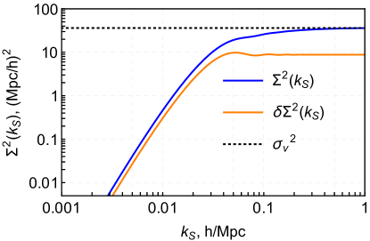
We plot the dependence of the damping factors and on the choice of in the left panel of Fig. 3. At small the damping functions have the following asymptotic behavior:
| (7.9) |
The integral in is cut off at by the Bessel function and becomes a constant equal to
| (7.10) |
whereas keeps growing up to Mpc where it approaches its asymptotic value . The integral in receives the dominant contribution from and is significantly bigger than . This numerical hierarchy is due to the specific shape of the CDM power spectrum which is strongly suppressed at ; if the power spectrum peaked at momenta smaller than , the damping factors and would have comparable magnitudes.
As discussed in Sec. 5.2, the scale should be chosen high enough to include the contributions of all relevant soft modes. At the same time, it should be smaller than the momentum of interest. In the numerical calculations below we will vary in the range Mpc. The dependence of the final result on the precise choice of should be considered as a measure of theoretical uncertainty.
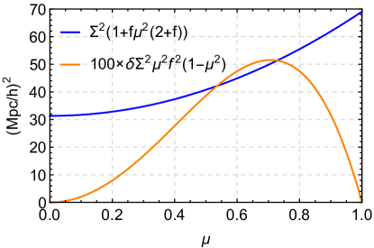
In order to understand the effect of damping in redshift space let us rewrite the expression (7.7) as with
| (7.11) |
and as functions of are plotted in the right panel of Fig. 3. We fix /Mpc. For visualization purposes we multiply by factor and flip its sign. We observe that is much smaller than for all wavevector directions. Its relative effect somewhat increases at high redshifts where the suppression by factor is mitigated. As for the contribution, we see that it grows monotonically with and thus, as expected, the BAO signal is more suppressed for the wavevectors aligned with the line-of-sight.
7.2 The power spectrum and bispectrum at next-to-leading order
At NLO the IR-resummed power spectrum can be written as
| (7.13) |
Note that the power spectrum that must be used as an input in the loop contribution is anisotropic due to the angular dependence of the damping factor. This complicates evaluation of the loop integral, as it prevents from using the standard procedure of integrating over the azimuthal angle and reducing to a finite series in . To cast (7.13) in a more convenient form, we isolate the wiggly terms,
| (7.14) |
where . The first term contains an integral of the isotropic smooth power spectrum and its evaluation does not pose any problem. The second term is an integral of a quickly oscillating function and is exponentially suppressed within our power counting. Indeed, approximating with the sine we have111111The kernel is not regular at . However, this singularity does not contribute because vanishes at the origin.,
| (7.15) |
Similarly, the hard part of the third integral, i.e. the contribution from , is also exponentially suppressed. On the other hand, in the vicinity the damping factor can be approximated as
| (7.16) |
The difference pertains to NLO soft corrections which we neglect in this paper. We conclude that the damping factor can be pulled out of the loop integrals without changing the order of approximation in our power counting. This allows us to rewrite the IR-resummed power spectrum in the form involving only integration over the isotropic initial power spectrum,
| (7.17) |
where is evaluated on the smooth power spectrum only and
| (7.18) |
An expression similar to (7.17) was obtained for the 1-loop IR resummed real-space power spectrum in Ref. [38].
For higher-point correlation functions the “isotropisation” of the IR resummed loop integrands is in general impossible. However, some partial contributions to the total result may still be simplified. Thus, in Appendix D we show that the 1-loop bispectrum in redshift space can be written in the following form,
| (7.19) |
where all terms except involve isotropic power spectra inside the momentum integrals. The ‘approximately equal’ sign between the first and second lines means that the two expressions are equal up to NLO soft correction. The formulae for , , and are given in Eqs. (D.5) of Appendix D.
7.3 Comparison with other approaches
Let us compare our results to other methods. At the phenomenological level the suppression of the BAO feature in redshift space is well described by a -dependent exponential damping acting on the wiggly part of the linear power spectrum. The aim of analytic approaches is to derive this result from first principles and consistently generalize it to higher orders in perturbation theory, where the effects beyond this simple damping are relevant. In this section we will focus on a few methods to describe the BAO peak which are most common in the literature.
The simplest model describing the suppression of the BAO peak in redshift space is given by
| (7.20) |
with two possible choices of the damping factor :
| (7.21a) | |||||
| (7.21b) | |||||
The model (7.20) explicitly takes into account the fact that bulk flows significantly affect only the wiggly part of the power spectrum. On the other hand, the damping factors in (7.21) are different from ours, given in Eq. (7.7). The rms velocity displacement in (7.21a) is enhanced at very low , whereas the modes with should not affect the BAO feature as dictated by the equivalence principle. On the other hand, the integrand (7.21b), as well as in our expressions (7.5), tends to zero in the IR, and thus is consistent with the physical expectations. The damping factor (7.21b) has the structure similar to our (7.5a) but is evaluated at . This choice of contradicts the logic that only long-wavelength modes should be resummed and should be contrasted with our expressions which explicitly reflect this argument. Indeed, only for the soft modes with the mode coupling affecting the BAO is enhanced.
As shown in Fig. 3, the numerical value of our damping factor appears to be quite close to both (7.21a) and (7.21b) for the CDM cosmology. It was already pointed out in [38, 35] that if our universe had more power at large scales, , the damping factor (7.7) would be notably different121212 It would be interesting to understand if this can account for the discrepancy between and the actual damping factor found in simulations of a toy cosmological model with a bigger in [80]. from . On the other hand, if there were more power at short scales, using (7.21b) one would significantly overdamp the BAO signal. Last but not least, the models (7.21) do not take into account the contribution, which, albeit small in the CDM cosmology, could be sizable if were smaller than .
The leading order IR-resummed power spectrum (7.6) coincides with the expression found in Ref. [81]. The approach used in [81] is related to the framework developed in Refs. [82, 83]. We point out that the accurate description of the BAO feature requires including loop corrections and thus goes beyond the simple exponential damping prescribed by (7.20).
Our results for the power spectrum are consistent with those obtained within the effective field theory of large scale structure [33, 41, 84, 85, 34, 36, 37]. Our expressions (5.35) and (LABEL:eq:PhNNLO) agree, up to higher order corrections131313Note that [84] essentially applies the operator to the whole power spectrum, including its smooth part. This is equivalent to a partial resummation of IR corrections to the smooth power spectrum. These corrections are not enhanced and therefore their resummation is not legitimate within our power-counting rules. , with those obtained in Ref. [84]. We emphasize that TSPT gives a simple diagrammatic description of IR resummation and provides a tool to examine and extend the results found in Ref. [84]. IR resummation in TSPT readily generalizes beyond the power spectrum and applies to any -point correlation functions with an arbitrary number of hard loops. The power counting, outlined in this paper, allows one to go beyond next-to-leading order in a systematic way. In particular, TSPT allows one to systematically compute the subleading soft corrections relevant for the shift of the BAO peak. We leave their detailed study for future work.
8 Numerical results and comparison with N-body data
In this section we show the results for the 2-point correlation function and the power spectrum of matter in redshift space, although our analysis can be easily extended to biased tracers. We will first discuss the 2-point correlation function, which allows us to clearly illustrate the effect of IR resummation on the BAO feature due to a better separation between the BAO peak and short scales. Then we compare our predictions for the IR-resummed power spectrum at one loop against N-body data. To the best of our knowledge, there are no publicly available data on the 2-point correlation function in redshift space. That is why in this paper we limit the comparison to the power spectrum, even though it is not optimal for the visualization of the BAO.
As common in redshift space analysis, we will study Legendre multipoles of the power spectrum and the 2-point correlation function, defined via141414 Recall that in our Fourier transform convention .
| (8.1) |
where is the Legendre polynomial of order . We will focus on the monopole, quadrupole and hexadecapole moments (), which fully characterize the linear correlation function in redshift space.
We consider the cosmological model corresponding to the N-body simulations performed in [78]. The linear power spectrum is produced with the Boltzmann code CLASS [86] and then decomposed into the wiggly and non-wiggly components using the spline approximation of the broadband power spectrum [35]. The redshift space one-loop integrals are evaluated using the FFTLog algorithm [87, 88]. A similar technique is used to compute the correlation function multipoles from those of the power spectrum.
8.1 2-point correlation function: quantitative study
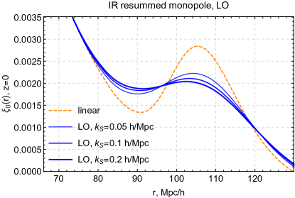
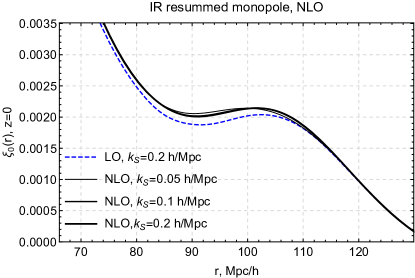
In the left panel of Fig. 4 we show the leading-order IR resummed monopole correlation function for three different values151515 Alternatively, one could consider a -dependent separation scale [38] to account for the fact that the enhancement only takes place for modes with . In order to avoid the uncertainty related to the precise form of -dependence, we prefer to keep as a free parameter that allows us to control the theoretical error of our method. of . For comparison we also show the prediction of linear theory. As expected, the damping of the BAO described by a simple exponential suppression of the wiggly component translates into a suppression of the BAO peak. On the other hand, the scatter induced by the choice of is quite sizable at leading order. To reduce this uncertainty one has to go to next-to-leading order. The corresponding correlation function is displayed in the right panel of Fig. 4. For comparison we also show the LO result for /Mpc. We observe that the 1-loop contribution slightly lifts the correlation function at short scales. The NLO predictions have a very mild (sub-percent) dependence on the separation scale which indicates the convergence of our resummation scheme.
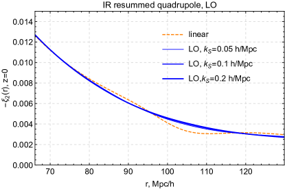
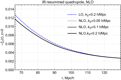
Fig. 5 shows the result for the quadrupole, . In the left panel we plot the correlation function in linear theory and at the leading order of IR resummation for three choices of . Since the quadrupole contribution is proportional to the derivatives of the real-space correlation function [49], instead of a single peak we observe an oscillating pattern at the BAO scales in linear theory. After IR resummation this pattern becomes almost invisible. This happens because the broadband part of the quadrupole has a significant amplitude at the BAO scale, which makes it difficult to distinguish a much smaller BAO contribution. We note that the dependence on the separation scale is quite mild both at leading (left panel) and next-to-leading order (right panel). We also observe the relative impact of the one-loop contribution becomes more sizable as compared to the monopole.
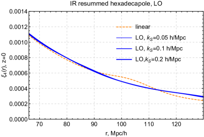
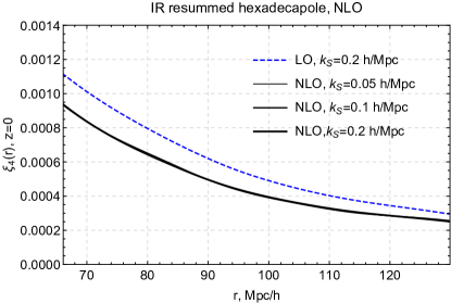
Fig. 6 shows the result for the hexadecapole, . Similarly to the previous case, we observe that the oscillating pattern corresponding to the BAO is strongly suppressed after the IR resummation. The dependence on the separation scale is mild both at LO and NLO. We observe that the broadband part is significantly altered by the one-loop correction to the smooth power spectrum.
8.2 Matter power spectrum: comparison with N-body data
In this section we compare our predictions for the power spectrum and its multipoles at LO and NLO with the N-body simulations performed in [78]. The results of this section should be taken with a grain of salt as they do not take into account UV counterterms whose inclusion is necessary for a consistent description of the short-scale dynamics. The analysis including UV counterterms will be reported elsewhere.
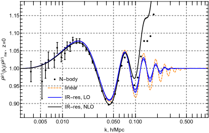
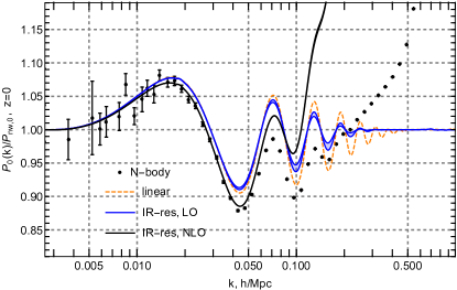
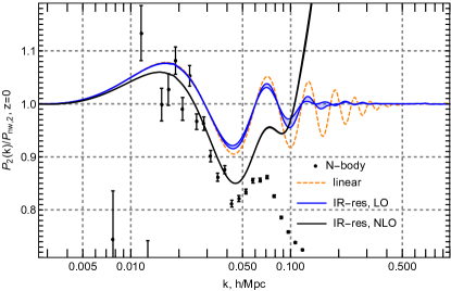
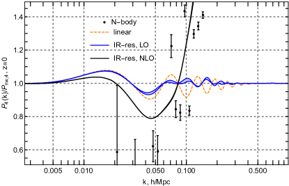
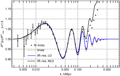
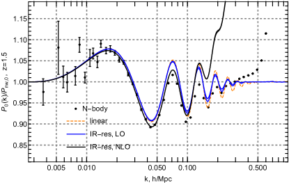
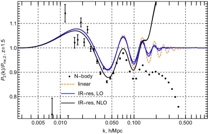
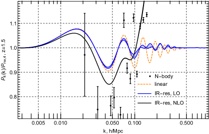
Fig. 7 shows the results for the power spectrum in real space at (upper left panel) and the power spectrum multipoles: monopole (upper right panel), quadrupole (lower left panel), and hexadecapole (lower right panel) divided by the corresponding linear non-wiggly power spectra. We show the predictions of linear theory (orange, dashed), leading order (blue) and next-to-leading order (black) IR resummation models. For IR resummed power spectra we show bands corresponding to the theoretical uncertainty caused by variation of in the range /Mpc. Note that for the NLO spectra this band is barely visible. The error bars correspond to sample variance from an overall simulation volume . They do not take into account systematic errors due to discreteness effects, which become big for higher-order power spectrum multipoles at large scales. In particular, we observe that the fluctuations in the measured hexadecapole power spectrum are very large even at mildly non-linear scales.
Qualitatively, we observe that the LO result does not improve much over linear theory as it misses the correct broadband information, while upon including the 1-loop corrections at NLO the agreement between the data and the theory improves. The monopole and quadrupole moments clearly exhibit the finger-of-God suppression at short scales. It reduces the range of agreement between the data and the theory as compared to real space and implies that UV counterterms should play a significant role is redshift space [85, 36].
In Fig. 8 we demonstrate the results for , which display an improvement in the agreement between the data and the theory over a wider range of scales in line with the suppression of non-linearities at large redshifts.
9 Summary and outlook
In this paper we embedded redshift space distortions and bias in time-sliced perturbation theory. We developed a manifestly IR-safe framework which allows us to perturbatively compute non-linear equal-time correlation functions of biased tracers in redshift space. The key observation is that the coordinate transformation from real to redshift space can be viewed as a fictitious 1D fluid flow, which maps real space correlation functions to the redshift space ones. Once this mapping is done, one can systematically resum the enhanced IR corrections affecting the BAO feature. The IR resummation of cosmological correlators proceeds in a straightforward manner along the lines of [35]. IR resummation in TSPT is based on physically motivated power counting rules and has a clear diagrammatic representation, which allows to compute the relevant corrections in a systematic and controllable way.
Our analysis gives a simple prescription for the numerical evaluation of the IR-resummed cosmological correlation functions. First, one has to isolate the oscillating part of the power spectrum as only this contribution is susceptible to non-linear damping due to bulk flows. IR resummation at leading order amounts to replacing the usual linear power spectrum by the “improved” one,
| (9.1) |
where is the cosine of the angle between the wavevector and the line-of-sight, is the separation scale defining the range of modes which are resummed, and the damping factor is given in (7.5). Applying this prescription we obtained the explicit expressions for the IR-resummed power spectrum (7.6) and bispectrum (7.12) of biased tracers in redshift space.
At first order in hard loops IR resummation amounts to computing loop diagrams using the IR-resummed power spectrum (9.1) as an input. This must be accompanied by modification of the input power spectrum in the tree-level part to avoid double counting. The general formula for -point IR-resummed redshift-space correlator reads,
| (9.2) |
where and are the tree-level and 1-loop contributions understood as functionals of the input power spectrum. Equation (9.2) applies both to the density and velocity correlators, as well as to biased tracers. It also admits a straightforward generalization to higher orders in hard loops.
The angular dependence of the damping factor in (9.2) reduces the symmetry of one-loop integrands and complicates the numerical evaluation. We have shown that for the one-loop power spectrum it is possible to rearrange our result in an equivalent form, Eq. (7.17), suitable for numerical implementation using standard algorithms. We also derived a simplified expression for the redshift-space 1-loop bispectrum, see Eq. (7.19).
The separation scale is a priori arbitrary and any dependence on it should be considered as part of the theoretical uncertainty. We show that the scatter of our results w.r.t variations of this scale in the reasonable range /Mpc is not negligible at LO, but substantially reduces when including NLO corrections. This testifies the convergence of our resummation procedure.
We compared our results with available N-body data on the power spectrum of matter in redshift space and found that IR resummation at NLO significantly improves the range of agreement between theory and data compared to linear theory and LO IR resummation. The results of our comparison are preliminary at the moment as we have not included into calculation the UV-counterterms. Taking into account these counterterms is expected to further improve the agreement. We leave this task for future study.
Our results suggest several directions for future research. On one hand, one can accurately assess the shift of the BAO peak in redshift space and for biased tracers. Although the expression (7.17) already contains some contributions into the shift, its precise value must be validated by computing full NLO soft corrections. On the other hand, our results may be useful for elucidating systematic uncertainties of the reconstruction algorithms, see Ref. [24] for a recent work in this direction. Finally, our theoretical template may be used for analyzing the data from full-shape measurements of galaxy clustering without reconstruction.
Acknowledgments
We are grateful to V. Assassi, D. Blas, H. Gil-Marín, F. Schmidt, M. Schmittfull, G. Trevisan and M. Zaldarriaga for illuminating discussions. We are indebted to Z. Vlah for sharing with us his numerical results and for valuable comments. We thank M. Simonović for help with the FFTLog algorithm and for encouraging interest. We are grateful to D. Blas and M. Garny for useful comments on the draft. This work is supported by the Swiss National Science Foundation. M.I. also acknowledges a partial support by the RFBR grant No. 17-02-01008. S.S. is supported by the RFBR grant No. 17-02-00651.
Appendix A Review of time-sliced perturbation theory for matter in real space
In this section we give a brief review of TSPT for matter in real space with emphasis on IR resummation [43, 35]. For clarity we will omit the superscripts in the notations for cosmological fields. We are interested in the correlation functions of the overdensity field and the velocity divergence field , whose time-evolution is governed by the continuity and Euler equations for the peculiar flow velocity ,
| (A.1a) | |||
| (A.1b) | |||
where and . Here is conformal time and is the matter density fraction. It is well-known [52] that in the case of an Einstein–de Sitter universe these equations can be cast in a form free from any explicit time dependence by introducing the time parameter , where is the linear growth factor, and appropriately rescaling the velocity divergence
| (A.2) |
with . For the realistic CDM cosmology, the substitution (A.2) into (A.1) leaves a mild residual time dependence which, however, has little effect on the dynamics. Following conventional practice we will neglect this explicit time dependence in the equations of motion, but keep the factor when it appears in redshift space quantities.
In Fourier space Eqs. (A.1) can be rewritten as
| (A.3) |
with non-linear kernels
| (A.4) |
The main idea of the TSPT approach is to substitute the time evolution of the overdensity and velocity divergence fields, and , by that of the their time dependent probability distribution functional. This idea is particularly useful when one is only interested in equal time correlation functions. For adiabatic initial conditions only one of the two fields is statistically independent. We choose it to be the velocity divergence field and denote its probability distribution functional by . At any moment in time, the field can be expressed in terms of as
| (A.5) |
with . Equation (A.5) can be used to eliminate the density field from Eq. (A.1) and obtain a closed equation for the velocity divergence,
| (A.6) |
with corresponding to the growing mode in the perfect fluid approximation. The kernels and are found recursively using the relations,
| (A.7a) | |||
| (A.7b) | |||
| (A.7c) | |||
| (A.7d) | |||
Equal-time correlation functions for and can be obtained by taking functional derivatives with respect to the external sources and , respectively, of the following partition function,
| (A.8) |
The probability density functional satisfies the Liouiville equation which reflects the conservation of probability,
| (A.9) |
In perturbation theory one can represent (logarithm of) as a power series in ,
| (A.10) |
where is a normalization factor. Substituting this representation into (A.9) and using Eq. (A.6) we obtain the following chain of equations on the vertices,
| (A.11) |
It is convenient to decompose the solution of these equations into two pieces:
| (A.12) |
where is the solution of the homogeneous equations (A.11) with the initial conditions reflecting the initial statistical distribution, and is the solution of the inhomogeneous equations with vanishing initial conditions. The vertices have the physical meaning of 1-particle irreducible tree-level correlators with amputated external propagators, and are counterterms, whose role is to cancel divergences in the loop corrections [43].
For the Gaussian initial conditions the time-dependence of the vertices factorizes,
| (A.13) |
where the time-independent kernels are given by
| (A.14a) | |||
| (A.14b) | |||
The counterterms do not depend on time and are given by:
| (A.15a) | |||
A.1 IR resummation in real space
IR resummation in real-space TSPT proceeds in three steps [35]:
1. One notices that the vertices are functionals of the linear power spectrum . Hence, the decomposition of into the smooth and wiggly parts induces a similar decomposition of the vertices,
| (A.16) |
where the terms are neglected.
2. One identifies IR-enhanced contributions. These are characterized by inverse powers of the small parameter , where is a soft (loop) momentum and is an external momentum. The enhancement takes place only for the wiggly vertices which have the following asymptotic behavior in the limit :
| (A.17) |
where the operator acts on the wiggly power spectrum as follows,
| (A.18) |
From (A.18) we see that the wiggly vertex is enhanced as
| (A.19) |
3. One introduces power counting rules and resum all the contributions at a desired order. The power counting rules in real and redshift spaces are the same, see Sec. 5.2. The procedure of IR resummation in TSPT has a simple diagrammatic interpretation. The leading soft corrections correspond to daisy diagrams with multiple soft loops dressing a single wiggly vertex. This is true irrespective of the number of hard loops in the diagram. The soft loop contributions factorize, which allows to easily resum them to all orders in perturbation theory. For a generic wiggly vertex with hard wavenumbers dressed by soft loops one has
| (A.20) |
Using Eq. (A.17) we obtain
| (A.21) |
Clearly, the summation over the number of soft loops leads to an exponentiation of the differential operator
| (A.22) |
For we obtain
| (A.23) |
Adding the smooth part and inverting the whole vertex we obtain the LO result for the power spectrum
| (A.24) |
Approximating the differential operator as (7.2) leads to
| (A.25) |
where the damping factor is given in Eq. (7.5a) and we have switched to the compact notation for the time-dependent linear power spectrum (7.1). IR resummation at first order in hard loops amounts to evaluating the loop integrals using (A.24) and accounting for double counting in the tree-level result, e.g. for the power spectrum we have
| (A.26) |
This procedure generalizes to higher point functions , i.e.
| (A.27) |
These expressions are valid up to next-to-leading order soft corrections which are numerically small.
Appendix B Asymptotic behavior of RSD vertices in the soft limit
In this Appendix we prove the asymptotic formula (5.13) for the redshift space vertices. For clarity we will omit the superscript in the notation for the wiggly vertices and keep in mind that these quantities are evaluated in redshift space. In what follows it is useful to define the operator
| (B.1) |
To prove (5.13) we proceed by induction. In Eq. (5.7) we have verified this formula for . Now, suppose it is valid for and any . Our aim is to prove it for . Using the recursion relation (4.9) we write
| (B.2) |
where we have introduced a shorthand notation . Let us estimate the enhancement of various terms in this expression. The real-space vertex is of order , as seen from Eq. (A.17). The vertices in the second and third lines have soft arguments and thus are also enhanced as according to our induction hypothesis. The vertices in the last three lines have one soft argument less and thus are only . In the fourth and fifth lines, however, this is compensated by the poles in the kernels,
| (B.3) |
Keeping only the terms we arrive at
| (B.4) |
Next, we use that due to momentum conservation and rewrite the last two terms as
| (B.5) |
On the other hand, the first term in square brackets in (B.4) reads,
| (B.6) |
where in the last equality we again used the relation (4.9). Combining Eqs. (B.5) and (B.6) we obtain,
| (B.7) |
Integration and use of Eq. (A.17) for the real space vertex yields the formula (5.13). QED
Appendix C Bias expansion at one loop
In order to obtain the bias kernels at one loop we have to go to the second order in , i.e. we need only
| (C.1) |
At first order there is a single operator in the bias expansion, . At second order there are two operators,
| (C.2) |
At third order we have:
| (C.3) |
Going into Fourier space and using the decomposition (A.5) we obtain (6.12) with the following kernels:
| (C.4) |
where ‘perm.’ means terms obtained by cyclic permutations of the momenta . Note that the kernels written above are manifestly IR safe. The kernels in redshift space are obtained using the recursion relations similar to (4.17). In particular, we have
| (C.5) |
where . The expression for is rather cumbersome and we do not present it here.
For reference we also write down the SPT kernels for biased tracers in redshift space. Compared to [52] we add the tidal bias. It appears convenient to change the bias basis and consider
| (C.6) |
where
| (C.7) |
and we introduced we velocity potential defined via . Acting along the lines of Sec. 7.4.1 of [52] we obtain
| (C.8a) | |||
| (C.8b) | |||
| (C.8c) | |||
where and the kernel must be symmetrized in its arguments.
Appendix D Simplification of NLO IR resummed integrands: example of bispectrum in redshift space
At face value, IR resummation requires using the dressed anisotropic power spectrum
| (D.1) |
as an input in loop calculations. This prescription causes technical complications that one would like to minimize. We have seen in Sec. 7.2 that in the case of one-loop power spectrum one can pull the anisotropic damping factor outside the momentum integral without changing the order of approximation of the final result. Here we discuss the general situation for an 1-loop -point correlator and illustrate it on the example of bispectrum. We will work in terms of SPT diagrams.
Consider an SPT one-loop diagram for some -point function and substitute the linear power spectrum in it by its IR-resummed counterpart (D.1). Depending on the topology of the diagram the wiggly power spectrum can be:
-
(a)
outside the loop and depend only on an external momentum. In this case the loop integral contains only the isotropic smooth power spectrum and its evaluation is straightforward.
-
(b)
inside the loop and be multiplied by a combination of kernels without IR singularities at finite values of the loop momentum (we choose to coincide with the argument of ). An example of such contribution is given by the second term in (7.14) which is part of diagram in SPT language. As we discussed in Sec. 7.2, such contributions are exponentially suppressed and can be safely neglected.
-
(c)
inside the loop and be multiplied by a combination of kernels with a single IR singularity at , where is a linear combinations of external momenta. This is the case of the third term in (7.14) which comes from the diagram. In such diagram the argument of the damping factor can be substituted by ,
(D.2) Then the damping factor can be taken out of the loop integral.
-
(d)
inside the loop and be multiplied by a combination of kernels with more than one IR singularity. We are not aware of any convenient method to simplify these contributions, so in this case the anisotropic damping factor must be kept inside the integral.
Applying the above algorithm to the one-loop correction to the bispectrum we obtain the following expression,
| (D.3) |
where is evaluated using only the smooth power spectrum and
| (D.4) |
Here the individual terms read,
| (D.5a) | |||
| (D.5b) | |||
| (D.5c) |
References
- [1] D. J. Eisenstein et al. [SDSS Collaboration], Astrophys. J. 633, 560 (2005) [astro-ph/0501171].
- [2] S. Cole et al. [2dFGRS Collaboration], Mon. Not. Roy. Astron. Soc. 362, 505 (2005) [astro-ph/0501174].
- [3] S. Alam et al. [BOSS Collaboration], Mon. Not. Roy. Astron. Soc. 470, no. 3, 2617 (2017) [arXiv:1607.03155 [astro-ph.CO]].
- [4] T. M. C. Abbott et al. [DES Collaboration], “Dark Energy Survey Year 1 Results: Measurement of the Baryon Acoustic Oscillation scale in the distribution of galaxies to redshift 1,” [arXiv:1712.06209 [astro-ph.CO]].
- [5] T. Delubac et al. [BOSS Collaboration], Astron. Astrophys. 574, A59 (2015) [arXiv:1404.1801 [astro-ph.CO]].
- [6] J. E. Bautista et al., Astron. Astrophys. 603, A12 (2017) [arXiv:1702.00176 [astro-ph.CO]].
- [7] M. Ata et al., Mon. Not. Roy. Astron. Soc. 473, no. 4, 4773 (2018) [arXiv:1705.06373 [astro-ph.CO]].
- [8] J. Hou et al., “The clustering of the SDSS-IV extended Baryon Oscillation Spectroscopic Survey DR14 quasar sample: anisotropic clustering analysis in configuration-space,” arXiv:1801.02656 [astro-ph.CO].
- [9] Y. Liang, C. Zhao, C. H. Chuang, F. S. Kitaura and C. Tao, Mon. Not. Roy. Astron. Soc. 459, no. 4, 4020 (2016) [arXiv:1511.04391 [astro-ph.CO]].
- [10] C. Zhao, C. H. Chuang, Y. Liang, F. S. Kitaura, M. Vargas-Magaña, C. Tao, M. Pellejero-Ibanez and G. Yepes, arXiv:1802.03990 [astro-ph.CO].
- [11] Z. Slepian et al., Mon. Not. Roy. Astron. Soc. 468, no. 1, 1070 (2017) [arXiv:1512.02231 [astro-ph.CO]].
- [12] Z. Slepian et al., Mon. Not. Roy. Astron. Soc. 469, no. 2, 1738 (2017) [arXiv:1607.06097 [astro-ph.CO]].
- [13] D. W. Pearson and L. Samushia, “A Detection of the Baryon Acoustic Oscillation Features in the SDSS BOSS DR12 Galaxy Bispectrum,” arXiv:1712.04970 [astro-ph.CO].
- [14] D. J. Eisenstein, H. j. Seo, E. Sirko and D. Spergel, Astrophys. J. 664, 675 (2007) [astro-ph/0604362].
- [15] H. J. Seo et al., Astrophys. J. 720, 1650 (2010) [arXiv:0910.5005 [astro-ph.CO]].
- [16] M. Schmittfull, Y. Feng, F. Beutler, B. Sherwin and M. Y. Chu, Phys. Rev. D 92, no. 12, 123522 (2015) [arXiv:1508.06972 [astro-ph.CO]].
- [17] A. Obuljen, F. Villaescusa-Navarro, E. Castorina and M. Viel, JCAP 1709, no. 09, 012 (2017) [arXiv:1610.05768 [astro-ph.CO]].
- [18] H. M. Zhu, Y. Yu, U. L. Pen, X. Chen and H. R. Yu, Phys. Rev. D 96, no. 12, 123502 (2017) [arXiv:1611.09638 [astro-ph.CO]].
- [19] H. M. Zhu, U. L. Pen and X. Chen, “Primordial density and BAO reconstruction,” arXiv:1609.07041 [astro-ph.CO].
- [20] M. Schmittfull, T. Baldauf and M. Zaldarriaga, Phys. Rev. D 96, no. 2, 023505 (2017) [arXiv:1704.06634 [astro-ph.CO]].
- [21] F. Beutler et al. [BOSS Collaboration], Mon. Not. Roy. Astron. Soc. 464, no. 3, 3409 (2017) [arXiv:1607.03149 [astro-ph.CO]].
- [22] A. J. Ross et al. [BOSS Collaboration], Mon. Not. Roy. Astron. Soc. 464, no. 1, 1168 (2017) [arXiv:1607.03145 [astro-ph.CO]].
- [23] M. Peloso, M. Pietroni, M. Viel and F. Villaescusa-Navarro, JCAP 1507, no. 07, 001 (2015) [arXiv:1505.07477 [astro-ph.CO]].
- [24] Z. Ding, H. J. Seo, Z. Vlah, Y. Feng, M. Schmittfull and F. Beutler, “Theoretical Systematics of Future Baryon Acoustic Oscillation Surveys,” arXiv:1708.01297 [astro-ph.CO].
- [25] D. Baumann, D. Green and M. Zaldarriaga, JCAP 1711, no. 11, 007 (2017) [arXiv:1703.00894 [astro-ph.CO]].
- [26] D. Baumann, F. Beutler, R. Flauger, D. Green, M. Vargas-Magaña, A. Slosar, B. Wallisch and C. Yèche, “First Measurement of Neutrinos in the BAO Spectrum,” arXiv:1803.10741 [astro-ph.CO].
- [27] F. Beutler et al. [BOSS Collaboration], Mon. Not. Roy. Astron. Soc. 466, no. 2, 2242 (2017) [arXiv:1607.03150 [astro-ph.CO]].
- [28] S. Satpathy et al. [BOSS Collaboration], Mon. Not. Roy. Astron. Soc. 469, no. 2, 1369 (2017) [arXiv:1607.03148 [astro-ph.CO]].
- [29] M. Crocce and R. Scoccimarro, Phys. Rev. D 73, 063519 (2006) [astro-ph/0509418].
- [30] M. Crocce and R. Scoccimarro, Phys. Rev. D 77, 023533 (2008) [arXiv:0704.2783 [astro-ph]].
- [31] D. J. Eisenstein, H. j. Seo and M. J. White, Astrophys. J. 664, 660 (2007) [astro-ph/0604361].
- [32] T. Matsubara, Phys. Rev. D 77, 063530 (2008) [arXiv:0711.2521 [astro-ph]].
- [33] L. Senatore and M. Zaldarriaga, JCAP 1502, no. 02, 013 (2015) [arXiv:1404.5954 [astro-ph.CO]].
- [34] Z. Vlah, U. Seljak, M. Y. Chu and Y. Feng, JCAP 1603, no. 03, 057 (2016) [arXiv:1509.02120 [astro-ph.CO]].
- [35] D. Blas, M. Garny, M. M. Ivanov and S. Sibiryakov, JCAP 1607, no. 07, 028 (2016) [arXiv:1605.02149 [astro-ph.CO]].
- [36] L. F. de la Bella, D. Regan, D. Seery and S. Hotchkiss, JCAP 1711, no. 11, 039 (2017) [arXiv:1704.05309 [astro-ph.CO]].
- [37] L. Senatore and G. Trevisan, “On the IR-Resummation in the EFTofLSS,” arXiv:1710.02178 [astro-ph.CO].
- [38] T. Baldauf, M. Mirbabayi, M. Simonovic and M. Zaldarriaga, Phys. Rev. D 92, no. 4, 043514 (2015) [arXiv:1504.04366 [astro-ph.CO]].
- [39] M. Mirbabayi, M. Simonovic and M. Zaldarriaga, “Baryon Acoustic Peak and the Squeezed Limit Bispectrum,” arXiv:1412.3796 [astro-ph.CO].
- [40] T. Matsubara, Phys. Rev. D 78, 083519 (2008) Erratum: [Phys. Rev. D 78, 109901 (2008)] [arXiv:0807.1733 [astro-ph]].
- [41] L. Senatore and M. Zaldarriaga, “Redshift Space Distortions in the Effective Field Theory of Large Scale Structures,” arXiv:1409.1225 [astro-ph.CO].
- [42] Z. Vlah, E. Castorina and M. White, JCAP 1612 (2016) no.12, 007 [arXiv:1609.02908 [astro-ph.CO]].
- [43] D. Blas, M. Garny, M. M. Ivanov and S. Sibiryakov, JCAP 1607, no. 07, 052 (2016) [arXiv:1512.05807 [astro-ph.CO]].
- [44] J. C. Jackson, Mon. Not. Roy. Astron. Soc. 156, 1P (1972) [arXiv:0810.3908 [astro-ph]].
- [45] W. L. W. Sargent and E. L. Turner, Astrophys. J. Lett. 212, L3-L7 (1977).
- [46] R. B. Tully and J. R. Fisher, “Nearby small groups of galaxies,” The large scale structure of the universe; Proceedings of the Symposium, Tallin, Estonian SSR, September 12-16, 1977. (A79-13511 03-90) Dordrecht, D. Reidel Publishing Co., 1978, p. 31-45; Discussion, p. 45-47.
- [47] E. Jennings, C. M. Baugh and S. Pascoli, Mon. Not. Roy. Astron. Soc. 410, 2081 (2011) [arXiv:1003.4282 [astro-ph.CO]].
- [48] N. Kaiser, Mon. Not. Roy. Astron. Soc. 227, 1 (1987).
- [49] A. J. S. Hamilton, Astrophys. J. 385, L5 (1992).
- [50] J. A. Peacock and S. J. Dodds, Mon. Not. Roy. Astron. Soc. 267, 1020 (1994) [astro-ph/9311057].
- [51] M. Pietroni, JCAP 0810, 036 (2008) [arXiv:0806.0971 [astro-ph]].
- [52] F. Bernardeau, S. Colombi, E. Gaztanaga and R. Scoccimarro, Phys. Rept. 367, 1 (2002) [astro-ph/0112551].
- [53] R. Scoccimarro and J. Frieman, Astrophys. J. Suppl. 105, 37 (1996) [astro-ph/9509047].
- [54] P. Creminelli, J. Noreña, M. Simonović and F. Vernizzi, JCAP 1312, 025 (2013) [arXiv:1309.3557 [astro-ph.CO]].
- [55] E. T. Vishniac, MNRAS 203, 345 (1983).
- [56] B. Jain and E. Bertschinger, Astrophys. J. 456 (1996) 43 [astro-ph/9503025].
- [57] D. Blas, M. Garny and T. Konstandin, JCAP 1309, 024 (2013) [arXiv:1304.1546 [astro-ph.CO]].
- [58] J. J. M. Carrasco, S. Foreman, D. Green and L. Senatore, JCAP 1407 (2014) 056 [arXiv:1304.4946 [astro-ph.CO]].
- [59] N. S. Sugiyama and D. N. Spergel, JCAP 1402 (2014) 042 [arXiv:1306.6660 [astro-ph.CO]].
- [60] A. Kehagias and A. Riotto, Nucl. Phys. B 873 (2013) 514 [arXiv:1302.0130 [astro-ph.CO]].
- [61] M. Peloso and M. Pietroni, JCAP 1305 (2013) 031 [arXiv:1302.0223 [astro-ph.CO]].
- [62] D. Baumann, A. Nicolis, L. Senatore and M. Zaldarriaga, JCAP 1207, 051 (2012) [arXiv:1004.2488 [astro-ph.CO]].
- [63] J. J. M. Carrasco, M. P. Hertzberg and L. Senatore, JHEP 1209, 082 (2012) [arXiv:1206.2926 [astro-ph.CO]].
- [64] B. D. Sherwin and M. Zaldarriaga, Phys. Rev. D 85, 103523 (2012) [arXiv:1202.3998 [astro-ph.CO]].
- [65] N. Kaiser, Astrophys. J. 284, L9 (1984).
- [66] P. McDonald and A. Roy, JCAP 0908, 020 (2009) [arXiv:0902.0991 [astro-ph.CO]].
- [67] T. Baldauf, U. Seljak, L. Senatore and M. Zaldarriaga, JCAP 1110, 031 (2011) [arXiv:1106.5507 [astro-ph.CO]].
- [68] L. Senatore, JCAP 1511, no. 11, 007 (2015) [arXiv:1406.7843 [astro-ph.CO]].
- [69] M. Mirbabayi, F. Schmidt and M. Zaldarriaga, JCAP 1507, no. 07, 030 (2015) [arXiv:1412.5169 [astro-ph.CO]].
- [70] R. Angulo, M. Fasiello, L. Senatore and Z. Vlah, JCAP 1509, no. 09, 029 (2015) [arXiv:1503.08826 [astro-ph.CO]].
- [71] V. Desjacques, D. Jeong and F. Schmidt, “Large-Scale Galaxy Bias,” arXiv:1611.09787 [astro-ph.CO].
- [72] V. Assassi, D. Baumann, D. Green and M. Zaldarriaga, JCAP 1408, 056 (2014) [arXiv:1402.5916 [astro-ph.CO]].
- [73] U. Seljak, JCAP 1203, 004 (2012) [arXiv:1201.0594 [astro-ph.CO]].
- [74] V. Desjacques, D. Jeong and F. Schmidt, “The Galaxy Power Spectrum and Bispectrum in Redshift Space,” arXiv:1806.04015 [astro-ph.CO].
- [75] J. E. McEwen, X. Fang, C. M. Hirata and J. A. Blazek, JCAP 1609, no. 09, 015 (2016) [arXiv:1603.04826 [astro-ph.CO]].
- [76] X. Fang, J. A. Blazek, J. E. McEwen and C. M. Hirata, JCAP 1702, no. 02, 030 (2017) [arXiv:1609.05978 [astro-ph.CO]].
- [77] D. Bertolini, K. Schutz, M. P. Solon, J. R. Walsh and K. M. Zurek, Phys. Rev. D 93, no. 12, 123505 (2016) [arXiv:1512.07630 [astro-ph.CO]].
- [78] H. Gil-Marin, C. Wagner, L. Verde, C. Porciani and R. Jimenez, JCAP 1211, 029 (2012) [arXiv:1209.3771 [astro-ph.CO]]. The data are available at http://icc.ub.edu/hector/Hector_Gil_Marin/Public.html
- [79] H. J. Seo and D. J. Eisenstein, Astrophys. J. 665, 14 (2007) [astro-ph/0701079].
- [80] N. Padmanabhan and M. White, Phys. Rev. D 80, 063508 (2009) [arXiv:0906.1198 [astro-ph.CO]].
- [81] T. Nishimichi, E. Noda, M. Peloso and M. Pietroni, JCAP 1801, no. 01, 035 (2018) [arXiv:1708.00375 [astro-ph.CO]].
- [82] M. Peloso and M. Pietroni, JCAP 1701, no. 01, 056 (2017) [arXiv:1609.06624 [astro-ph.CO]].
- [83] E. Noda, M. Peloso and M. Pietroni, JCAP 1708, no. 08, 007 (2017) [arXiv:1705.01475 [astro-ph.CO]].
- [84] M. Lewandowski, L. Senatore, F. Prada, C. Zhao and C. H. Chuang, Phys. Rev. D 97, no. 6, 063526 (2018) [arXiv:1512.06831 [astro-ph.CO]].
- [85] A. Perko, L. Senatore, E. Jennings and R. H. Wechsler, “Biased Tracers in Redshift Space in the EFT of Large-Scale Structure,” arXiv:1610.09321 [astro-ph.CO].
- [86] D. Blas, J. Lesgourgues and T. Tram, JCAP 1107, 034 (2011) [arXiv:1104.2933 [astro-ph.CO]].
- [87] A. J. S. Hamilton, Mon. Not. Roy. Astron. Soc. 312, 257 (2000) [astro-ph/9905191].
- [88] M. Simonovic, T. Baldauf, M. Zaldarriaga, J. J. Carrasco and J. A. Kollmeier, JCAP 1804, no. 04, 030 (2018) [arXiv:1708.08130 [astro-ph.CO]].