Gluon poles and photon distribution amplitudes in Drell-Yan-like processes

Abstract

We calculate the hadron tensor related to the photon-induced Drell-Yan process, with incoming nucleon being transversally polarised. We predict the new single spin asymmetry which probes gluon poles and which is expressed in terms of photon (both chiral-odd and chiral-even) distribution amplitudes and chiral-odd nucleon function stemming from the nucleon transverse polarization.

I Introduction

In experimental studies, the single spin asymmetry (SSA) is a useful tool for such kind of investigations. In particular, the single transverse spin asymmetry gives a lot of information on the three-dimensional nucleon structure owing to the nontrivial connection between the nucleon transverse spin and the transverse momentum dependence of parton distributions (see, for example, Angeles-Martinez:2015sea ; Boer:2011fh ; Boer:2003cm ; Kang:2011hk ; Boer:2011fx ; Arnold:2008kf ). Among the semi-inclusive reactions, the Drell-Yan-like (DY-like) processes play an unique role due to a possibility to uncover the gluon pole contributions and to study finest structure of hadron transverse polarization effects Anikin:2010wz ; Anikin:2015xka ; Anikin:2015esa ; Anikin:2017azc ; Anikin:2017vvn ; Anikin:2017pch .

Moreover, there are several experimental projects which pursue the measurements with Drell-Yan-like processes, RHIC Bai:2013plv , COMPASS Baum:1996yv ; COMPASS and future NICA Kouznetsov:2017bip ; Savin:2016arw .

As well-known, the DY-like processes with an essential transverse polarization of nucleons give a possibility to explore the gluon poles in the twist-$3$ quark-gluon parton distribution functions (PDFs), denoted as $B^{V}$-PDFs in, for instance, Anikin:2010wz ; Anikin:2015xka ; Anikin:2015esa . In Ref. Anikin:2017azc , based on the duality properties, the twist-$3$ $B^{V}$-PDF has been modelled by the corresponding convolution of two hadron distribution amplitudes. This model has allowed to study the gluon pole presence in more detail and it has resulted in the prediction of new SSAs related to the pion-induced DY process which are reachable for measurements by COMPASS COMPASS .

Here, we propose a new study of the DY-like processes where the gluon poles lead in significant ways to to new SSA observables. In particular, we would like to focus our attention on the photon-induced DY process where the twist-$3$ photon distribution amplitudes (photon DAs) can be probed. Let us emphasise that the understanding of hadron-like behavior of photons, which is encoded in the photon DA, still attracts the attention of community Ioffe:1983ju ; Balitsky:1989ry ; Ball:2002ps ; Braun:2002en ; Berger:1979du . The attempt to study the leading twist-$2$ photon DA was implemented some years ago in Pire:2009ap .

In this paper we calculate the Drell-Yan hadron tensors related to the photon-nucleon processes with the essential spin transversity and “primordial” transverse momenta where the gluon poles have been shown up. We construct a new single spin asymmetry the existence of which entirely depends on the presence of gluon poles. We dwell on the case where one of photon DAs has been projected onto the twist-$2$ chiral-odd structure, $\langle\bar{\psi}\sigma^{+\perp}\psi\rangle$. We stress that the photon chiral-odd DA singles out the chiral-odd tensor combination in the nucleon matrix element with essential transverse polarization. Notice that, in this case, the access to the specific angular dependence of SSA (see Eqn. (18)) expressed in terms of the Collins-Soper angles has been opened only owing to the gluon pole presence. In other words, the experimental verification of SSA’s angular dependence predicted in the present paper can give evidences for the gluon pole probing and the hadron-like behaviour of photons.

II Kinematics

Let us now go over to the discussion of kinematics. We consider the photon-induced Drell-Yan process with nucleon being transversely polarized at the regime where Bjorken fraction $x_{B}$ is close to $1$, i.e. $x_{B}\to 1$ :

$$\gamma(P_{1})+N^{(\uparrow\downarrow)}(P_{2}) \to \gamma^{*}(q)+\bar{q}(K)+X(P_{X})$$

$$\to \bar{q}(K)+\ell(l_{1})+\bar{\ell}(l_{2})+X(P_{X}).$$

The virtual photon producing the lepton pair ($l_{1}+l_{2}=q$) has a large mass squared ($q^{2}\approx Q^{2}$) while its transverse momenta $q_{\perp}$ are small and integrated out.

The light-cone (Sudakov) decompositions supplemented with usual approximations take the forms Anikin:2017azc

$$P_{1}=\frac{Q}{x_{B}\sqrt{2}}\,n^{\star}-\frac{x_{B}P^{2}_{1\,\perp}}{Q\sqrt{2}}n+P_{1\,\perp}\approx\frac{Q}{x_{B}\sqrt{2}}\,n^{\star}+P_{1\,\perp}\,,$$

$$P_{2}\approx\frac{Q}{y_{B}\sqrt{2}}\,n+P_{2\,\perp}\,,\quad S\approx\frac{\lambda}{M_{2}}\,P_{2}+S_{\perp}\,$$ (2)

for the real photon and nucleon momenta and nucleon spin vector;

$$q=\frac{Q}{\sqrt{2}}\,n^{\star}+\frac{Q}{\sqrt{2}}\,n+q_{\perp},\,\quad q_{\perp}^{2}\ll Q^{2}\,,$$ (3)

for the virtual photon momentum. The momenta $P_{1}$ and $P_{2}$ have the plus and minus dominant light-cone components, respectively.

It is convenient to define the Collins-Soper frame, i.e. the center-mass-system of lepton pair, as Barone:2001sp

$$\widehat{t}=\frac{q}{Q},\quad\widehat{x}=\frac{q_{\perp}}{Q_{\perp}},\quad\widehat{z}=\frac{x_{B}}{Q}\widetilde{P}_{1}-\frac{y_{B}}{Q}\widetilde{P}_{2},$$ (4)

where $\widetilde{P}_{1}={P}_{1}-q/(2x_{B})$ and $\widetilde{P}_{2}={P}_{2}-q/(2y_{B})$ . Moreover, we have

$$\sqrt{2}n^{\star}=\widehat{t}+\widehat{z}-\frac{Q_{\perp}}{Q}\widehat{x},\quad\sqrt{2}n=\widehat{t}-\widehat{z}-\frac{Q_{\perp}}{Q}\widehat{x}.$$ (5)

III Hadron tensor

The processes (II) are studied in the kinematics with a large $Q^{2}$, so we apply the factorization theorem to get the corresponding hadron tensor factorized in the form where the hard part is convoluting with the soft part. All important steps of our factorization approach can be found, for instance, in Anikin:2010wz ; Anikin:2015xka ; Anikin:2015esa (see, also the references therein).

It is natural to study the role of observables at twist-$3$ level by exploring of different associated asymmetries. Any single spin asymmetries (SSAs) can be presented in the following symbolical form

$${\cal A}\sim d\sigma^{(\uparrow)}-d\sigma^{(\downarrow)}\sim{\cal L}_{\mu\nu}\,H_{\mu\nu}\,,$$ (6)

where ${\cal L}_{\mu\nu}$ is the corresponding leptonic tensor and $H_{\mu\nu}$ stands for the hadronic tensor. For our purposes, it is enough to consider the case of unpolarized leptons which leads to the real lepton tensor and, therefore, the hadron tensor $H_{\mu\nu}$ has to be real one too. As for any DY-like processes, the hadron tensor includes at least two non-perturbative blobs which are associated with two different dominant (plus and minus) light-cone directions. For the process (II), the hadron tensor involves the upper non-perturbative blob (see Figs. 1 and 2) which corresponds to the matrix elements with the spin transversity:

$$\langle P_{2},S_{\perp}|\bar{\psi}\,\sigma^{-\perp}\,\psi|S_{\perp},P_{2}\rangle\stackrel{{\scriptstyle{\cal F}}}{{\sim}}\varepsilon^{-\perp S^{\perp}P_{2}}\,\bar{h}.$$ (7)

Notice that the upper blob corresponds to the dominant minus light-cone direction and the dominant antiquark momentum $k_{2}$ is defined along the minus direction too. In more general case, the function $\bar{h}(y)$ can be expressed through the corresponding moments of the transverse momentum dependent functions.

In contrast to the usual DY-process (with two initial nucleons) with the twist-$3$ $B^{V}$-PDF Anikin:2010wz , in the photon-induced DY case the lower non-perturbative blob splits into two photon distribution amplitudes: the one of twist-$2$, $\langle\bar{\psi}\,\sigma^{+\perp}\psi\rangle$, and the second one of twist-$3$, $\langle\bar{\psi}\,\gamma^{\perp}\psi\rangle$ (in the similar way as for the pion-induced DY-process Anikin:2017azc ).

Generally speaking, the hadron tensor involves the contributions from two different kinds of amplitude interference, see Figs. 1 and 2, together with the mirror contributions. Moreover, the hadron tensor term which arises from such a interference contains the contributions from both the “standard” and “non-standard” diagrams as shown in Fig. 1 . As was explained in Anikin:2016bor , in this case the gluon propagator involves the transverse gluons only, i.e. with the the gluon propagator numerator $d_{\alpha\beta}(\ell)=g^{\perp}_{\alpha\beta}$. Thus, it is easy to see, by simple $\gamma$-algera, that for the lower blobs the convolution combination of $\langle\bar{\psi}\,\sigma^{+\perp}\psi\rangle$ and $\langle\bar{\psi}\,\gamma^{\perp}\psi\rangle$ as presented in Fig. 1 does not contribute to the hadron tensor at all.

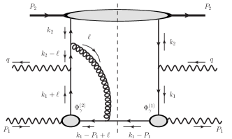
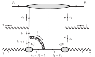
Figure 1: The “standard” diagram (the upper panel) and the “non-standard” diagram (the lower panel) do not contribute to the considered hadron tensor of photon-induced DY process.

Hence, we are left with the only possible interference which generates the hadron tensor shown in Fig. 2 which refers to the “standard” diagram. Note that the “non-standard” diagram vanishes in this case.

We are now in position to discuss the derivation of hadron tensor generated by the diagram in Fig. 2. As mentioned, we adhere the terminology and the collinear factorization procedure as described in Anikin:2010wz ; Anikin:2015xka ; Anikin:2015esa . The dominant quark and gluon momenta $k_{1}$ and $\ell$ lie along the plus direction while, as above-mentioned, the dominant antiquark momentum $k_{2}$ – along the minus direction (see Figs. 1 and 2). That is the behaviours of parton momenta on the light-cone satisfy the conditions:

$$k_{1}\,\,\text{and}\,\,\ell\sim\left(P_{1}^{+},\,\frac{\Lambda_{1}^{2}}{P^{+}_{1}},\,\Lambda_{1}\right),\quad k_{2}\sim\left(\frac{\Lambda_{2}^{2}}{P^{-}_{2}},P^{-}_{2},\Lambda_{2}\right),$$ (8)

where $\Lambda_{i}$ characterize the hadron typical scales.

Before factorization, this diagram leads to the following contribution (all prefactors are included in the integration measures)

$${\cal W}_{\mu\nu}=\int(d^{4}k_{1})\,(d^{4}k_{2})\,\delta^{(4)}(k_{1}+k_{2}-q)$$

$$\times\int(d^{4}\ell)\,{\cal D}_{\alpha\beta}(\ell)\text{tr}\big{[}\gamma_{\nu}\sigma^{+\perp}\gamma_{\alpha}\sigma^{-\perp}\gamma_{\mu}S(k_{1}+\ell-P_{1})\gamma_{\beta}\gamma^{\perp}\big{]}$$

$$\times\bar{\Phi}^{[\sigma^{-\perp}]}(k_{2})\,\Phi_{(2)\gamma}^{[\sigma^{+\perp}]}(k_{2};\ell)\,\Phi_{(1)\gamma}^{[\gamma^{\perp}]}(k_{1})\,\delta\big{(}(P_{1}-k_{1})^{2}\big{)}+$$

$$(\text{Fierz projection replacement}:[\sigma^{+\perp}]\leftrightarrow[\gamma^{\perp}])\,,$$ (9)

where

$${\cal D}_{\alpha\beta}(\ell)=\Delta(\ell)d_{\alpha\beta}(\ell),\quad\Delta(\ell)=\frac{1}{\ell^{2}+i0},$$ (10)

and

$$\bar{\Phi}^{[\sigma^{-\perp}]}(k_{2})=\int\sum\nolimits_{X}\,\int(d^{4}\eta_{2})\,e^{-ik_{2}\eta_{2}}\,$$ (11)

$$\times\langle P_{2},S_{\perp}|\text{tr}\big{[}\psi(0)|P_{X}\rangle\,\langle P_{X}|\bar{\psi}(\eta_{2})\sigma^{-\perp}\big{]}|S_{\perp},P_{2}\rangle\,$$

and

$$\Phi_{(2)\gamma}^{[\sigma^{+\perp}]}(k_{2};\ell)=i\,P_{1}^{+}e_{(\lambda)}^{\perp}\varphi^{(2)}_{\gamma}(k_{2},\ell)=$$ (12)

$$\int(d^{4}\eta_{1})\,e^{i(P_{1}+k_{2}-\ell)\eta_{1}}\,\langle 0|\bar{\psi}(\eta_{1})\,\sigma^{+\perp}\psi(0)|P_{1}\rangle\,,$$

$$\Phi_{(1)\gamma}^{[\gamma^{\perp}]}(k_{1})=e_{(\lambda)}^{\perp}\varphi^{(1)}_{\gamma}(k_{1})=$$ (13)

$$\int(d^{4}\xi)\,e^{-ik_{1}\xi}\,\langle P_{1}|\bar{\psi}(\xi)\,\gamma^{\perp}\psi(0)|0\rangle\,.$$

In Eqns. (12) and (13) the factors which include the quark condensate $\langle\bar{\psi}\psi\rangle$, the magnetic susceptibility $\chi$, and the non-perturbative constant $f_{3\gamma}$ are absorbed in the definitions of $\varphi^{(i)}_{\gamma}$ (see Ball:2002ps for details). In Eqn. (III) we write explicitly the $\delta$-function which shows that the quark operator with the momentum $P_{1}-k_{1}$ corresponds to the on-shell fermion. Moreover, since we here deal with the only “standard” diagram, within the contour gauge $[z^{-};-\infty^{-}]_{A^{+}}=1$ (see, Anikin:2010wz ; Anikin:2015xka ; Anikin:2015esa ) which leads to the local axial gauge $A^{+}=0$, the gluon propagator in Eqn. (III) contains contributions of two contractions: $\langle A^{\perp}A^{\perp}\rangle$ and $\langle A^{\perp}A^{-}\rangle$. In other words, the numerator $d^{\alpha\beta}(\ell)$ in Eqn. (10) receives the contributions from $d^{\perp\,\perp}(\ell)$ and $d^{\perp\,-}(\ell)$ combinations.

The next step is to perform the factorization procedure for the hadron tensor. We are not going to discuss details of factorization stages (the comprehensive description of factorization can be found in many papers, see, for example, An-ImF ; Belitsky:2005qn ; Diehl:2003ny ; Braun:2011dg ).

Figure 2: The Feynman diagrams which contribute to the photon-induced Drell-Yan hadron tensor.

By referring to Anikin:2017azc , in the limit $x_{B}\to 1$, we finally derive the following expression for the gauge invariant hadron tensor (here, $x_{21}=x_{2}-x_{1}$):

$$\overline{\cal W}_{\mu\nu}=\int d^{2}\vec{\bf q}_{\perp}{\cal W}_{\mu\nu}=$$ (14)

$$=i\,\frac{s^{2}}{4}\int(dx_{1})\,(dy)\,\delta(x_{1}P^{+}_{1}-q^{+})\delta(yP^{-}_{2}-q^{-})\Phi^{(1)}_{\gamma}(x_{1})$$

$$\times\int(dx_{2})\int(dk_{2}^{+}d^{2}\vec{\bf k}_{2}^{\perp})\bar{h}(y|k_{2}^{+},\vec{\bf k}_{2}^{\perp})\Phi^{(2)}_{\gamma}(y,x_{21}|k_{2}^{+},\vec{\bf k}_{2}^{\perp})\,$$

$$\times\frac{1}{2x_{21}}\left[g_{\mu\nu}^{\perp}\,(e^{(\lambda)}_{\perp}\cdot e^{*\,(\lambda)}_{\perp})-e^{(\lambda)}_{\perp\,\nu}\,e^{*\,(\lambda)}_{\perp\,\mu}-e^{(\lambda)}_{\perp\,\mu}\,e^{*\,(\lambda)}_{\perp\,\nu}\right]\varepsilon^{P_{1}^{\perp}S_{\perp}n^{\star}n},$$

where

$$\Phi^{(2)}_{\gamma}(y,x_{21}|k_{2}^{+},\vec{\bf k}_{2}^{\perp})=\int(d\ell^{-}d^{2}\vec{\ell}_{\perp})\frac{\vec{\ell}_{\perp}\cdot\vec{\bf P}_{1}^{\perp}}{(\vec{\bf P}_{1}^{\perp})^{2}}$$ (15)

$$\times\Phi^{(2)}_{\gamma}(y,x_{21}|k_{2}^{+},\vec{\bf k}_{2}^{\perp};\ell^{-},\vec{\ell}_{\perp})\Delta(\ell^{-},\vec{\ell}_{\perp})\Delta(\ell^{-},\vec{\ell}_{\perp}-\vec{\bf P}_{1}^{\perp})$$

and $\Phi^{(i)}_{\gamma}(..)=\varphi^{(i)}_{\gamma}(..)/(2\bar{x}_{i}P_{1}^{+})$.

In Eqns. (14) and (15) we distinguish the arguments of functions $\Phi^{(2)}_{\gamma}$ and $\bar{h}$ in the dominant light-cone variables ($y,x_{21}$) and (sub)sub-dominant variables ($k_{2}^{+},\vec{\bf k}_{2}^{\perp};\ell^{-},\vec{\ell}_{\perp}$).

Let us now discuss the possible simplifications which can be applied for both the longitudinal and transverse momentum dependences of function $\Phi^{(2)}_{\gamma}$. First, since this function is parametrizing the hadron matrix element with the photon carrying the momentum $P_{1}$ with the plus light-cone dominant component, it is clear that the momentum $k_{2}$ with the minus light-cone dominant component does not affect the dynamics of quark-(real)photon interaction. So, the simplest case of longitudinal momentum separation has been illustrated in Fig. 3.

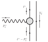
Figure 3: The longitudinal separable ansatz illustration.

The transverse momentum dependence separation, however, is more conditional. Within our frame, it is natural to assume that $|\vec{\ell}_{\perp}^{\,2}|\sim|\vec{\ell}_{\perp}\cdot\vec{\bf k}_{2}^{\perp}|\sim|\vec{\bf k}_{2\,\perp}^{\,2}|\sim O(1)$. Then, we can impose the separable ansatz in the form

$$\Phi^{(2)}_{\gamma}(y,x_{21}|k_{2}^{+},\vec{\bf k}_{2}^{\perp};\ell^{-},\vec{\ell}_{\perp})$$

$$\approx\widetilde{\Phi}^{(2)}_{\gamma}(x_{21}|\vec{\ell}_{\perp})\varphi_{S}(y|\vec{\bf k}_{2}^{\perp})+O\left(\frac{\ell^{-}}{P_{1}^{+}},\frac{k_{2}^{+}}{P_{2}^{-}}\right),$$ (16)

where $\varphi_{S}$ has a role of “spectator” function. Justification of the separability in Eqn. (III) can be demonstrated by using of the effective Lagrangian method in order to calculate the non-perturbative photon-vacuum matrix element of twist-$2$ quark operators which corresponds to $\Phi^{(2)}_{\gamma}$, see Appendix A.

Finally, we focus on discussion of the pole contribution $1/x_{21}$ in Eqn. (14). Similarly as in Ref. Anikin:2017azc , the gluon pole, which has to be treated within the contour gauge framework, can be described as Anikin:2010wz ; Anikin:2015xka ; Anikin:2015esa

$$\frac{1}{x_{2}-x_{1}}\stackrel{{\scriptstyle\text{c. g.}}}{{\Longrightarrow}}\frac{1}{x_{2}-x_{1}-i\epsilon}.$$ (17)

The complex prescription originates from the corresponding integral representation of theta function (see, Anikin:2015xka for details). This complex prescription in (17) generates the imaginary part in order to compensate the complex $i$ in parametrization of the photon-vacuum matrix element (12) and which leads to real part on the l.h.s. of (6).

IV Single Spin Asymmetry

We now construct the single spin asymmetry observable. Within the Collins-Soper frame Arnold:2008kf ; Barone:2001sp , performing the invariant integration in (14) and contracting the leptonic and hadron tensors, we finally obtain (we remind that ${\cal L}_{\mu\nu}$ corresponds the unpolarized lepton tensor)

$$\frac{4\,{\cal L}_{\mu\nu}\,\Im\text{m}\overline{\cal W}_{\mu\nu}}{Q^{2}}=\Phi^{(1)}_{\gamma}(x_{B})\,\widetilde{\Phi}^{(2)}_{\gamma}(\bar{x}_{B})\bar{h}(y_{B})\stackrel{{\scriptstyle\hskip 5.69046pt\vec{\bf k}_{2}^{\,\perp}}}{{\circledast}}\varphi_{S}(y_{B})$$ (18)

$$\times\frac{2}{x_{B}\,y_{B}}(e^{(\lambda)}_{\perp}\cdot e^{*\,(\lambda)}_{\perp})P_{1}^{\perp}\wedge S_{\perp}\,\sin^{2}\theta\cos 2\varphi,$$

where we use Eqn. (III) for $\Phi^{(2)}_{\gamma}$ and $\stackrel{{\scriptstyle\hskip 5.69046pt\vec{\bf k}_{2}^{\,\perp}}}{{\circledast}}$ stands for the corresponding integration over $\vec{\bf k}_{2}^{\,\perp}$ (cf. Eqn. (14)).

Therefore, we predict a new asymmetry which reads (cf. COMPASS )

$${\cal A}_{T}=\frac{S_{\perp}}{Q}\,\frac{D_{[\theta,\varphi]}\,\sin(\phi_{S}+\phi)C^{\sin\phi_{S}}_{UT}}{\bar{f}_{1}(y_{B})\,H_{1}(x_{B})},\,$$ (19)

$$D_{[\theta,\varphi]}=\frac{2\sin^{3}\theta\cos 2\varphi}{1+\cos^{2}\theta},$$ (20)

where $C^{\sin\phi_{S}}_{UT}=\Phi^{(1)}_{\gamma}(x_{B})\,\widetilde{\Phi}^{(2)}_{\gamma}(\bar{x}_{B})\bar{h}(y_{B})\stackrel{{\scriptstyle\hskip 5.69046pt\vec{\bf k}_{2}^{\,\perp}}}{{\circledast}}\varphi_{S}(y_{B})$; $\bar{f}_{1}(y_{B})$ and $H_{1}(x_{B})$ stem from the unpolarized cross-section and they parameterize the following matrix elements:

$$\langle P_{2}|\bar{\psi}\,\gamma^{-}\,\psi|P_{2}\rangle\stackrel{{\scriptstyle{\cal F}}}{{\sim}}P^{-}_{2}\bar{f}_{1}(y),\,$$

$$\langle P_{1}|\bar{\psi}_{+}|q(K)\rangle\langle q(K)|\psi_{+}|P_{1}\rangle\stackrel{{\scriptstyle{\cal F}}}{{\sim}}P_{1}^{+}H_{1}(x),$$ (21)

where

$$H_{1}(x)=\frac{1}{2\bar{x}P_{1}^{+}}\int(d^{2}\vec{\bf k}_{1}^{\,\perp})\varphi_{\gamma}^{(2)}(\bar{x},\vec{\bf k}_{1}^{\,\perp})\varphi_{\gamma}^{(1)}(x,\vec{\bf k}_{1}^{\,\perp}).$$

The new SSA defined by Eqn. (19) constitutes the main result of our study.

V Conclusion

We derive the gauge invariant photon-induced DY hadron tensor with the essential spin transversity and “primordial” transverse momenta. In the paper, we focus on the case where one of photon distribution amplitudes has been projected onto the chiral-odd twist-$2$ combination which singles out the chiral-odd parton distribution inside nucleons.

We predict a new single transverse spin asymmetry which can be probed experimentally and which are associated with the spin transversity and the nontrivial specific $\varphi$-angular dependence. This asymmetry can be treated as a signal of the gluon pole presence integrally with the study of both chiral-odd and chiral-even photon distribution amplitudes.

We emphasize that the possibility to study different SSAs induced by chiral-odd distribution functions/amplitudes appears only owing to the gluon pole presence. Thus, the proposed angular dependence of SSA can furnish the implicit evidences for the gluon pole observation in experiments.

Acknowledgments. We thank A.V. Efremov, L. Motyka, O.V. Teryaev and N. Volchanskiy for useful discussions. The work by I.V.A. was supported by the Bogoliubov-Infeld Program. I.V.A. also thanks the Theoretical Physics Division of NCBJ (Warsaw) for warm hospitality. L.Sz. is supported by grant No No 2017/26/M/ST2/01074 of the National Science Center in Poland.

Appendix A Demonstration of Separable Ansatz

In order to demonstrate the separable ansatz (III), it is instructive to estimate the non-perturbative matrix element which corresponds to the distribution amplitude within the frame of some effective model. A concrete realization of the model is not important for our purposes. So, we begin with the matrix element representing $\Phi^{(2)}_{\gamma}$ of the leading twist in the interaction representation. We have

$$M = \int(d^{4}\eta)e^{i(\ell-k_{2})\cdot\eta}\langle 0|T\bar{\psi}(0)\sigma^{+\perp}\psi(\eta)\mathbb{S}|P_{1}\rangle$$ (A.23)

$$= \int(d^{4}\eta)e^{i(\ell-k_{2})\cdot\eta}\int(d^{4}\xi)e^{-iP_{1}\cdot\xi}$$

$$\times\langle 0|T\bar{\psi}(0)\sigma^{+\perp}\psi(\eta)\frac{\delta\mathbb{S}}{\delta M(\xi)}|0\rangle,$$

where $\mathbb{S}$-matrix is given by the interaction action:

$$\mathbf{S}^{\text{eff.}}_{I}=g_{M}\int(d^{4}z)M(z)\bar{\psi}(z)\Gamma_{M}\psi(z).$$ (A.24)

Here, $M$ denotes the relevant meson which in our case is hadron-like photon. Note that, within the effective frame, the coupling constant $g_{M}$ can be calculated with a help of the bound (or coupling constant) condition (see for example Anikin:1995cf ; Anikin:2000th ). To the leading order of $g_{M}$, using the corresponding Fourier transformations, we obtain that

$$M=\text{tr}\left[\sigma^{+\perp}S(\ell-k_{2})\Gamma_{M}S(\ell-k_{2}-P_{1})\right].$$ (A.25)

In the paper, we study the hadron-like behaviour of photon, therefore we can choose $\Gamma_{M}=\sigma^{+\perp}$. With this choice and within the frame (II), we have

$$M=\frac{\text{tr}\left[\sigma^{+\perp}(\ell^{+}\gamma^{-})\sigma^{+\perp}([\ell^{+}-P^{+}_{1}]\gamma^{-})\right]}{\left[(\ell-k_{2})^{2}+i0\right]\left[(\ell-P_{1}-k_{2})^{2}+i0\right]}=\frac{\text{tr}\left[\sigma^{+\perp}\gamma^{-}\sigma^{+\perp}\gamma^{-}\right]}{\left[-2k_{2}^{-}-(\vec{\ell}_{\perp}-\vec{\bf k}_{2}^{\perp})^{2}/\ell^{+}+i\epsilon\right]\left[-2k_{2}^{-}-(\vec{\ell}_{\perp}-\vec{\bf k}_{2}^{\perp})^{2}/(\ell^{+}-P^{+}_{1})+i\epsilon\right]}$$ (A.26)

Let us now focus on the typical function which can be extracted from Eqn. (A.26)

$$\varphi((\vec{\ell}_{\perp}-\vec{\bf k}_{2}^{\perp})^{2})=\frac{1}{\left[-2k_{2}^{-}-(\vec{\ell}_{\perp}-\vec{\bf k}_{2}^{\perp})^{2}/\ell^{+}+i\epsilon\right]}.$$ (A.27)

Provided $|\vec{\ell}_{\perp}^{\,2}|\sim|\vec{\ell}_{\perp}\cdot\vec{\bf k}_{2}^{\perp}|\sim|\vec{\bf k}_{2\,\perp}^{\,2}|\sim O(1)$, we can make an approximation

$$\varphi((\vec{\ell}_{\perp}-\vec{\bf k}_{2}^{\perp})^{2})=-\frac{1}{2k_{2}^{-}}\left[1-\frac{(\vec{\ell}_{\perp}-\vec{\bf k}_{2}^{\perp})^{2}}{2k_{2}^{-}\ell^{+}}+...\right]\approx-\frac{1}{2k_{2}^{-}}\left[1-\frac{\vec{\ell}^{\,2}_{\perp}-\vec{\bf k}^{2}_{2\,\perp}}{2k_{2}^{-}\ell^{+}}+...\right]\approx-\frac{1}{2k_{2}^{-}}\left[1-\frac{\vec{\ell}^{\,2}_{\perp}}{2k_{2}^{-}\ell^{+}}+...\right]\left[1+\frac{\vec{\bf k}^{2}_{2\,\perp}}{2k_{2}^{-}\ell^{+}}+...\right]$$

$$=-\frac{1}{2k_{2}^{-}}\varphi_{1}(\vec{\ell}^{\,2}_{\perp})\varphi_{2}(\vec{\bf k}^{2}_{2\,\perp}).$$ (A.28)

This chain of approximations supports the separable ansatz.

References

- (1) R. Angeles-Martinez et al., Acta Phys. Polon. B 46, 2501 (2015)
- (2) D. Boer et al., arXiv:1108.1713 [nucl-th].
- (3) D. Boer, P. J. Mulders and F. Pijlman, Nucl. Phys. B 667, 201 (2003)
- (4) Z. B. Kang, J. W. Qiu, W. Vogelsang and F. Yuan, Phys. Rev. D 83, 094001 (2011)
- (5) D. Boer, Phys. Lett. B 702, 242 (2011)
- (6) S. Arnold, A. Metz and M. Schlegel, Phys. Rev. D 79, 034005 (2009)
- (7) I. V. Anikin and O. V. Teryaev, Phys. Lett. B 690, 519 (2010)
- (8) I. V. Anikin and O. V. Teryaev, Eur. Phys. J. C 75, no. 5, 184 (2015)
- (9) I. V. Anikin and O. V. Teryaev, Phys. Lett. B 751, 495 (2015)
- (10) I. V. Anikin, L. Szymanowski, O. V. Teryaev and N. Volchanskiy, Phys. Rev. D 95, no. 11, 111501 (2017)
- (11) I. V. Anikin, L. Szymanowski, O. V. Teryaev and N. Volchanskiy, J. Phys. Conf. Ser. 938, no. 1, 012065 (2017)
- (12) I. V. Anikin, L. Szymanowski, O. V. Teryaev and N. Volchanskiy, J. Phys. Conf. Ser. 938, no. 1, 012039 (2017)
- (13) M. Bai et al., “Status and Plans for the Polarized Hadron Collider at RHIC,”
- (14) G. Baum et al. [COMPASS Collaboration], CERN-SPSLC-96-14, CERN-SPSLC-P-297.
- (15) M. Aghasyan et al. [COMPASS Collaboration], arXiv:1704.00488 [hep-ex].
- (16) O. Kouznetsov and I. Savin, Nucl. Part. Phys. Proc. 282-284, 20.
- (17) I. Savin et al., Eur. Phys. J. A 52, no. 8, 215 (2016).
- (18) B. L. Ioffe and A. V. Smilga, Nucl. Phys. B 232, 109 (1984).
- (19) I. I. Balitsky, V. M. Braun and A. V. Kolesnichenko, Nucl. Phys. B 312, 509 (1989).
- (20) P. Ball, V. M. Braun and N. Kivel, Nucl. Phys. B 649, 263 (2003) [hep-ph/0207307].
- (21) V. M. Braun, S. Gottwald, D. Y. Ivanov, A. Schafer and L. Szymanowski, Phys. Rev. Lett. 89, 172001 (2002)
- (22) E. L. Berger and S. J. Brodsky, Phys. Rev. Lett. 42, 940 (1979).
- (23) B. Pire and L. Szymanowski, Phys. Rev. Lett. 103, 072002 (2009)
- (24) V. Barone, A. Drago and P. G. Ratcliffe, Phys. Rept. 359, 1 (2002)
- (25) I. V. Anikin, I. O. Cherednikov and O. V. Teryaev, Phys. Rev. D 95, no. 3, 034032 (2017)
- (26) I. V. Anikin, D. Y. Ivanov, B. Pire, L. Szymanowski and S. Wallon, Nucl. Phys. B 828, 1 (2010)
- (27) A. V. Belitsky and A. V. Radyushkin, Phys. Rept. 418, 1 (2005)
- (28) M. Diehl, Phys. Rept. 388, 41 (2003)
- (29) V. M. Braun and A. N. Manashov, JHEP 1201, 085 (2012)
- (30) I. V. Anikin, M. A. Ivanov, N. B. Kulimanova and V. E. Lyubovitskij, Z. Phys. C 65, 681 (1995).
- (31) I. V. Anikin, A. E. Dorokhov, A. E. Maksimov, L. Tomio and V. Vento, Nucl. Phys. A 678, 175 (2000).