Shell-model interactions from chiral effective field theory

Abstract

We construct valence-space Hamiltonians for use in shell-model calculations, where the residual two-body interaction is based on symmetry principles and the low-momentum expansion from chiral effective field theory. In addition to the usual free-space contact interactions, we also include novel center-of-mass–dependent operators that arise due to the Galilean invariance breaking by in-medium effects. We fitted the low-energy constants to 441 ground- and excited-state energies in the $sd$ shell and obtained a root-mean-square derivation of 1.8 MeV at leading order and of 0.5 MeV at next-to-leading order, with natural low-energy constants in all cases. The developed chiral shell-model interactions enable order-by-order uncertainty estimates and show promising predictions for neutron-rich isotopes beyond the fitted data set.

I Introduction

The nuclear shell model Brown (2001); Caurier et al. (2005); Coraggio et al. (2009) is a very successful many-body method, which is widely used for calculations of nuclear-structure properties in the medium to medium-heavy mass region of the nuclear chart. Typically, the model space for shell-model calculations includes one major harmonic-oscillator (HO) shell, or extensions by including another full shell or some of the lowest-lying subshells. In order to perform calculations in the nuclear shell model, one requires an effective Hamiltonian that describes the interactions among nucleons in the valence space under consideration.

There are two common approaches to develop valence-space Hamiltonians, which typically consist of single-particle energies (SPEs) and two-body matrix elements (TBMEs). First, there are very successful phenomenological approaches, where an effective interaction is constructed in a specific valence space by fitting free parameters to experimental properties in the model space. These are usually theoretically motivated based on a renormalized realistic interaction, where the TBMEs (or combinations thereof) and SPEs are then used to fine-tune the interaction, as in the universal $sd$-shell (USD) interactions of Ref. Brown and Richter (2006). This strategy (see, e.g., Refs. Brown (2001); Caurier et al. (2005) for reviews) typically leads to shell-model interactions that reproduce the experimental data with a root-mean-square (RMS) deviation of only a few hundred keV.

Second, valence-space Hamiltonians can be derived using modern ab initio methods, which can then be used in shell-model calculations. Among those methods are many-body perturbation theory (MBPT) Hjorth-Jensen et al. (1995); Coraggio et al. (2009); Holt et al. (2014); Simonis et al. (2016), the no-core shell model (NCSM) Dikmen et al. (2015); Barrett et al. (2013), coupled-cluster theory (CC) Jansen et al. (2014, 2016); Hagen et al. (2014) and the in-medium similarity renormalization group (IM-SRG) Tsukiyama et al. (2012); Bogner et al. (2014); Stroberg et al. (2017); Hergert et al. (2016). All of these methods start from a few-body Hamiltonian, which typically consists of two- and three-body interactions from chiral effective field theory (EFT). These methods do not achieve the same overall accuracy as the phenomenological fits, but they can provide uncertainty estimates.

In this paper, we use chiral EFT as a general operator basis at low energies and its capability to estimate theoretical uncertainties due to the EFT expansion to develop chiral shell-model interactions, where the low-energy couplings (LECs) are fit directly to data in the $sd$ shell. Chiral EFT provides a systematic expansion of strong interactions at low energies based on general symmetry principles in terms of nucleon and pion degrees of freedom Epelbaum et al. (2009); Machleidt and Entem (2011). Following Weinberg’s power counting Weinberg (1990, 1991), chiral EFT predicts a hierarchy of two- and many-body interactions governed by an expansion in powers of $(Q/\Lambda_{b})^{\nu}$ with order $\nu\geqslant 0$, were $Q$ is a generic low-momentum scale or the pion mass $m_{\pi}$ and $\Lambda_{b}\sim 500$ MeV is the breakdown scale of the EFT. Chiral EFT includes two-nucleon interactions at leading order (LO, $Q^{0}$) and many-body interactions start at next-to-next-to-leading order (N²LO, $Q^{3}$).

Because the pion-exchange interactions describe long-range physics, which is not renormalized in the medium, we take the long-range pion-exchange contributions directly as in free-space nuclear forces Epelbaum et al. (2009); Machleidt and Entem (2011). The short-range contact interactions encode physics beyond the degrees of freedom resolved in the EFT and therefore, for chiral shell-model interactions we fit these directly to data in the $sd$ shell. However, in the valence space, the presence of the core breaks Galilean invariance, and therefore novel short-range operators are possible that depend on the two-body center-of-mass (CM) momentum (or on the CM orbital angular momentum). These have been explored in the context of Fermi liquid theory in Ref. Schwenk and Friman (2004) and include operators that are known as antisymmetric spin-orbit interactions in the context of the shell model (see, e.g., Ref. Conze et al. (1973)). They enter at next-to-leading order (NLO, $Q^{2}$) in Weinberg counting, and we explore them for the first time in shell-model interactions.

In this work, we construct valence-space Hamiltonians in the $sd$ shell based on chiral EFT operators up to NLO. We fit the LECs to 441 ground- and excited-state energies in this model space. The LECs absorb in-medium effects due to the truncation of the model space. We will show the significance of the novel CM-dependent operators by constructing a full valence-space (vs) NLO interaction, which we label NLO_vs, and comparing it to results for a NLO interaction that uses only free-space operators from chiral EFT. We also compare our chiral shell-model interactions with the USD interactions from Ref. Brown and Richter (2006). Moreover, we explore order-by-order uncertainty estimates and show promising predictions for neutron-rich isotopes beyond the fitted data set.

This paper is organized as follows: In Sec. II, we discuss the free-space contact interactions and introduce the new CM-dependent operators at NLO. The partial-wave decomposition of the operators is given in App. A. The second part of Sec. II discusses the transformation to TBMEs in a HO basis and regulator aspects. Details on the transformation are given in App. B. We discuss specifics on the fitting process and give an overview of the quality of our fits in Sec. III. In Sec. IV, we show our results and predictions for ground-state energies and spectra, including estimates of the theoretical uncertainties. Finally, we summarize and give an outlook in Sec. V.

II Valence-shell interactions

II.1 Operators from chiral EFT

Following Weinberg’s power counting Weinberg (1990, 1991), there are two LECs at LO and seven new LECs at NLO. The LO and NLO contact interactions have the following form in momentum space:

$$\braket{\textbf{p}}{\bm{\mathrm{V}}_{\text{cont}}^{(\mathrm{LO})}}{\textbf{p}^{\prime}}=C_{S}+C_{T}\,\bm{\sigma}_{1}\cdot\bm{\sigma}_{2}\,,$$ (1)

and

$$\braket{\textbf{p}}{\bm{\mathrm{V}}_{\text{cont}}^{(\mathrm{NLO})}}{\textbf{p}^{\prime}} =C_{1}\textbf{q}^{2}+C_{2}\textbf{k}^{2}+\left(C_{3}\textbf{q}^{2}+C_{4}\textbf{k}^{2}\right)\bm{\sigma}_{1}\cdot\bm{\sigma}_{2}$$

$$+C_{5}\,\frac{\text{i}}{2}\left(\bm{\sigma}_{1}+\bm{\sigma}_{2}\right)\cdot\left(\textbf{q}\times\textbf{k}\right)$$

$$+C_{6}\left(\bm{\sigma}_{1}\cdot\textbf{q}\right)\left(\bm{\sigma}_{2}\cdot\textbf{q}\right)+C_{7}\left(\bm{\sigma}_{1}\cdot\textbf{k}\right)\left(\bm{\sigma}_{2}\cdot\textbf{k}\right),$$ (2)

where p and $\textbf{p}^{\prime}$ are the final and initial relative momenta with $\textbf{p}=(\textbf{p}_{1}-\textbf{p}_{2})/2$, q is the momentum transfer $\textbf{q}=\textbf{p}-\textbf{p}^{\prime}$ and k is the average momentum $\textbf{k}=(\textbf{p}+\textbf{p}^{\prime})/2$. The partial-wave decomposition of the free-space contact interactions is given in App. A.1.

The additional operators in the valence space, due to broken Galilean invariance by the presence of the core, depend explicitly on the two-body CM momentum $\textbf{P}=\textbf{p}_{1}+\textbf{p}_{2}$. We count powers of P as powers of $Q$, as they are set by the same scale (the inverse oscillator length) in a shell-model basis. Thus, the first contributions from these operators arise at NLO. We label the CM-dependent part of the contact interactions as NLO_vs, where vs is short for valence space. These take the following form in momentum space:

$$\braket{\textbf{p},\textbf{P}}{\bm{\mathrm{V}}_{\text{cont}}^{(\mathrm{NLO}_{\mathrm{vs}})}}{\textbf{p}^{\prime},\textbf{P}} =P_{1}\textbf{P}^{2}+P_{2}\textbf{P}^{2}\bm{\sigma}_{1}\cdot\bm{\sigma}_{2}$$

$$+P_{3}\,\text{i}\left(\bm{\sigma}_{1}-\bm{\sigma}_{2}\right)\cdot\left(\textbf{q}\times\textbf{P}\right)$$

$$+P_{4}\left(\bm{\sigma}_{1}\times\bm{\sigma}_{2}\right)\cdot\left(\textbf{k}\times\textbf{P}\right)$$

$$+P_{5}\left(\bm{\sigma}_{1}\cdot\textbf{P}\right)\left(\bm{\sigma}_{2}\cdot\textbf{P}\right)\,.$$ (3)

The CM-dependent interactions include central parts, given by the LECs $P_{1}$ and $P_{2}$, the difference- and cross-vector operators determined by $P_{3}$ and $P_{4}$, and a CM tensor operator, given by $P_{5}$. The latter three have been introduced and discussed in the context of noncentral interactions in Fermi liquid theory Schwenk and Friman (2004). As shown by the partial-wave decomposition in App. A.2, the central and tensor parts are diagonal in two-body spin $s$, relative orbital angular momentum $l$, and total (relative plus spin) angular momentum $j$, and they only contribute to the relative ${}^{1}S_{0}$ and ${}^{3}S_{1}$ waves. Note that in the presence of local regulators, regulator artifacts would also lead to contributions in higher partial waves (see, e.g., Ref. Huth et al. (2017)). Moreover, the central parts are diagonal in CM angular momentum $L$.

The difference- and cross-vector operators are spin-violating Schwenk and Friman (2004) and mix spin-singlet ${}^{1}S_{0}$ (${}^{1}P_{1}$) with spin-triplet ${}^{3}P_{j}$ (${}^{3}S_{1}$) relative partial waves. At NLO_vs, they do not contribute to higher $l$ waves. As a result of the $S$-$P$ mixing and parity conservation, the spin-violating interactions also change the CM angular momentum $L,L^{\prime}$ and are not necessarily diagonal in $j,j^{\prime}$. In the shell-model context, their structure is similar to the anti-symmetric spin-orbit interaction (see, e.g., Ref. Conze et al. (1973)).

In order to investigate the impact of the different CM-dependent interactions, we use in the following the notation NLO${}_{\mathrm{vs}_{c,v,t}}$ when only central, only vector, or only tensor operators are included, respectively.

II.2 Transformation to HO basis and regulators

In order to apply the momentum-space interactions in the valence space, we transform them to antisymmetrized, normalized two-body HO states. As detailed in App. B, this leads to TBMEs of the form

$$\braket{(n_{1}l_{1}j_{1})(n_{2}l_{2}j_{2})JT}{V}{(n^{\prime}_{1}l^{\prime}_{1}j^{\prime}_{1})(n^{\prime}_{2}l^{\prime}_{2}j^{\prime}_{2})JT},$$ (4)

where $(n_{i},l_{i},j_{i})$ are the single-particle radial, orbital angular momentum, and total angular momentum quantum numbers, and $J,T$ are the two-body total angular momentum and isospin, respectively.

The radial HO wave functions are given by

$$R_{nl}(p)=N_{nl}\,(pb)^{l}\,\exp\Bigl{[}-\frac{1}{2}(pb)^{2}\Bigr{]}L_{n}^{l+\frac{1}{2}}\Bigl{(}(pb)^{2}\Bigr{)}\,,$$ (5)

and are plotted in Fig. 1 for different $n,l$ quantum numbers relevant for $sd$-shell TBMEs. The oscillator length $b=\sqrt{\hbar/(m\omega)}$ is used with $\hbar\omega=13.53$ MeV to reproduce the radius of the ¹⁶O core. For completeness, the normalization is $N_{nl}=b^{3/2}\sqrt{2n!/\Gamma(n+l+3/2)}$ and $L_{n}^{l+\frac{1}{2}}$ are generalized Laguerre polynomials.

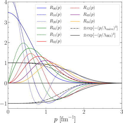
Figure 1: Radial wave functions relevant for $sd$-shell TBMEs in comparison to typical regulators used in chiral EFT with the naive cutoff estimate $\Lambda_{\mathrm{naive}}=300\,\mathrm{MeV}$ and $\Lambda_{\mathrm{HO}}=375\,\mathrm{MeV}$. See text for details.

Figure 1 shows that the radial wave functions involved in a limited valence space automatically cut off the high-momentum parts, and therefore no additional momentum-space regulator functions are necessary. In fact, one can naively estimate the cutoff in energy due to the basis truncation by

$$\frac{\Lambda_{\mathrm{naive}}^{2}}{m_{N}}\sim E\leqslant\varepsilon_{1}+\varepsilon_{2}=2(N_{\mathrm{valence}}+3/2)\hbar\omega\,.$$ (6)

For the $sd$ shell it follows that $\Lambda_{\mathrm{naive}}\approx 300\,\mathrm{MeV}$. A more sophisticated estimate is given in Ref. König et al. (2014) leading to a cutoff estimate for the $sd$ shell $\Lambda_{\mathrm{HO}}\approx 375\,\mathrm{MeV}$. In Fig. 1, we also compare the radial wave functions relevant for $sd$-shell TBMEs with commonly used regulators from chiral EFT with the two cutoff estimates described above. We observe that the radial wave functions indeed have a similar behavior in the high-momentum part as the regulator function with $\Lambda_{\mathrm{HO}}=375\,\mathrm{MeV}$. Hence, there is no necessity for additional momentum-space regulator functions for the contact interactions.

III Fit

III.1 Data set

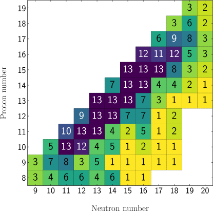
Figure 2: Graphical representation of the 441 experimental states used in our $sd$-shell fits. Each square shows the number of states fitted for a given isotope, where the color coding gets darker with increasing number of states.

With the LO and different NLO operators in place, the next step is to determine the LECs by fits to experimental data. For our data set, we consider 441 out of the 608 states that were used for the USDA/USDB fits Brown and Richter (2006). This set is smaller than the one used for USDA/USDB, because we included at most 12 excited states for a given isotope. The number of states we fit to each isotope is visualized in Fig. 2. As in Ref. Brown and Richter (2006), we apply a proton number dependent Coulomb correction to the experimental ground-state energies, so that we can focus on the strong interaction part. The Coulomb corrections used are listed in Table 1.

Table 1: Coulomb correction for a given proton number $Z$ from Ref. Brown and Richter (2006). We have corrected the experimental ground-state energies by subtracting the Coulomb correction.

$Z$	element	Coulomb correction [MeV]
08	Oe	00.00
09	Fe	03.48
10	Ne	07.45
11	Na	11.73
12	Mg	16.47
13	Al	21.48
14	Si	26.78
15	Pe	32.47
16	Se	38.46
17	Cl	44.74
18	Ar	51.31
19	Ke	58.14

III.2 Optimization

As mentioned above, the HO frequency is set by the ¹⁶O radius. For different mass number $A$, we apply a scaling factor $(18/A)^{1/3}$ to the TBMEs to correct the HO frequency for larger nuclei, which is a standard procedure in shell-model calculations. Our SPEs are set to reproduce the one-neutron separation energy and the first two excited states of ¹⁷O. The LECs of the contact operators are then determined by a $\chi^{2}$ minimization. The $\chi^{2}$ value per datum is calculated as follows:

$$\chi^{2}=\frac{1}{N-p}\sum\limits_{i=1}^{N}\left(\frac{E^{\text{exp}}_{i}-E^{\text{th}}_{i}}{\sigma_{i}}\right)^{2},$$ (7)

where $N$ is the total number of states and $p$ the number of parameters (LECs) in the fit. The experimental energy $E^{\text{exp}}_{i}$ is taken from the data set mentioned above, and the theoretical result $E^{\text{th}}_{i}$ is obtained by diagonalizing the valence-space Hamiltonian. For this, we use the shell-model code ANTOINE Caurier and Nowacki (1999); Caurier et al. (2005). The uncertainty $\sigma_{i}$ is given by $\sigma_{i}^{2}=(\sigma_{i}^{\text{exp}})^{2}+(\sigma_{i}^{\text{th}})^{2}$, where we take the experimental uncertainty from the data set and for the theoretical uncertainty we use a constant value $\sigma_{i}^{\text{th}}=0.1\,\mathrm{MeV}$ as in Ref. Brown and Richter (2006). In future work, we will also propagate the uncertainty from the EFT expansion, which we explore here first after the fits in Sec. IV.1. For the optimization, we use the linear combination method, described in Ref. Brown and Richter (2006). The routine shows a fast and stable convergence, but requires a linear dependence on our LECs, which rules out uncertainty estimates that explicitly depend on the parameters. We have also checked that the fit is stable under further optimization with POUNDerS algorithm Munson et al. ; Wild et al. (2015) or using the Nelder-Mead method Nelder and Mead (1965). Finally, we have considered several starting points for the fits: all LECs set to zero; starting from LECs fit to reproduce the USDA/B interactions; and starting from LECs fit to reproduce MBPT TBME from chiral NN+3N interactions. We have observed that the fits based on these starting points all lead to the same minimum.

As our theoretical uncertainty has no statistical interpretation, neither does the resulting $\chi^{2}$ value, and thus, we rather compare the RMS deviation to experiment for different interactions. The RMS deviation is given by

$$\text{RMS}=\sqrt{\frac{1}{N}\sum\limits_{i=1}^{N}\left(E^{\text{exp}}_{i}-E^{\text{th}}_{i}\right)^{2}}\,.$$ (8)

III.3 Overview of comparison with experiment

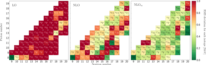
Figure 3: Graphical representation of the RMS deviation from experiment for each fitted nucleus in the $sd$ shell. The figure shows the results for the chiral shell-model interactions at LO (left), NLO (middle), and NLO_vs(right). The color coding of the RMS deviation is given in the bar on the right. Isotopes with a small RMS deviation are colored green, while those with a large deviation are colored red. Each square shows the isotope label and the number of fitted states in the bottom right corner. The text color changes from black to white for RMS deviations larger than 0.7 MeV.

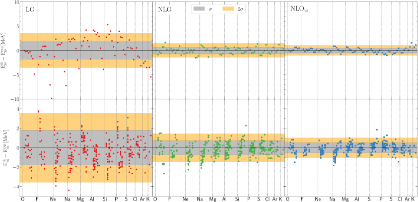
Figure 4: Energy differences of the result from the chiral shell-model interactions and experiment in MeV. The upper row shows results for ground-state (gs) energies whereas the lower row is for the energies of excited (ex) states. Each dot represents a single state. The dots are ordered from oxygen to potassium, and within each bin they are ordered according to their mass number. From left to right, we show results for the LO, NLO, and NLO_vs interaction. The gray (orange) bands show the statistical $\sigma$ ($2\sigma$) spread, given by the RMS deviation.

In Fig. 3 we show the RMS deviation from experiment for each fitted nucleus in the $sd$ shell for the chiral shell-model interactions at LO (left), NLO (middle), and NLO_vs (right). The RMS deviation is given by a color coding that ranges from 0 MeV (green) to 1 MeV (red). The results show a striking improvement from LO to NLO and a further improvement from NLO to NLO_vs, where at NLO_vs, there are only a few outliers with large RMS deviations. This demonstrates the impact of the new CM-dependent operators.

We also show a quantitative overview of the comparison with experiment in Fig. 4. The figure is divided into two rows, where the upper row shows the difference between theoretical and experimental ground-state energies and the lower row is for the difference between theoretical and experimental excitation energies. The columns show again the results for the LO (left), NLO (middle), and NLO_vs (right) shell-model interactions. The gray (orange) bands show the $\sigma$ ($2\sigma$) intervals given by the RMS deviation. The order-by-order improvement from LO to NLO and from NLO to NLO_vs, already seen globally in Fig. 3, is clearly visible from the decreasing $\sigma$ bands from left to right and from the systematically decreasing individual energy differences. Overall, we observe a very good reproduction of experiment at NLO_vs.

The results for the ground-state energies at LO in Fig. 4 show a systematic deviation from experiment with increasing neutron richness, especially for the oxygen to silicon isotopes, where the LO shell-model interaction leads to overbound states with respect to experiment. This trend seems to be resolved at NLO, where no clear pattern is visible. However, at NLO_vs, there is again a deficiency in the isospin dependence for the neon to aluminum isotopic chains. It will be interesting to see whether this will be improved at N²LO, and whether this can be traced back to the inclusion of three-nucleon forces Otsuka et al. (2010a), which enter at N²LO.

Systematic trends of this type are not visible in the energy differences for the excited states in Fig. 4. Note that the number of excited states is higher for nuclei close to stability (see also Fig. 2), so that there are more points shown at the beginning of each element in Fig. 4. However, it stands out that there is little to no improvement in the first two sodium isotopes (²²Na and ²³Na) from NLO to NLO_vs, which exemplary shows that additional operator structures are necessary to reach higher accuracies in the fit.

III.4 Comparison to USD-type interactions

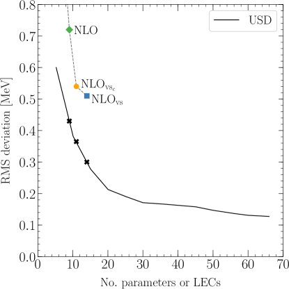
Figure 5: Root-mean-square deviation of the chiral and USD-type interactions as a function of the number of parameters. The results for the USD fit are taken from Ref. Brown and Richter (2006). The figure shows the free-space operator NLO interaction (green diamond), the NLO${}_{\mathrm{vs_{\mathrm{c}}}}$ interaction including only the central CM-dependent operators in addition to NLO (yellow circle), and the full NLO_vs shell-model interactions (blue square).

In addition to the direct comparison with experiment, we study how the developed chiral shell-model interactions perform compared to USD-type interactions, where the TBMEs are not determined by a basis of operators but are fit overall. The RMS deviation of the USD fit is taken from Fig. 4 of Ref. Brown and Richter (2006) and is shown as solid line as a function of the number of parameters in Fig. 5. Note that the USD fit was to a data set with 608 states, while our results are for the data set of 441 states described above, so the comparison is not completely one-to-one.

In Fig. 5, we plot the RMS deviation as a function of the number of LECs for the different chiral shell-model interactions developed in this work. In order to assess the impact of the new CM-dependent operators, we also analyze the central (vs_c), vector (vs_v), and tensor (vs_t) contributions separately. The RMS deviations for all interactions and the number of LECs are given in Table 2. Note that in comparison to the RMS deviation for a given nucleus (see Fig. 3) or for ground- and excited states separately (see Fig. 4) the RMS deviations discussed here are with respect to the full data set considered. As shown in Table 2, the RMS deviation improves 1.8 MeV at LO to 0.7 MeV at NLO and 0.5 MeV at NLO_vs.

To guide the comparison with the USD-type interactions in Fig. 5, the latter are marked by a cross for 9, 11, and 14 parameters, which corresponds to the same number of LECs as the NLO, NLO${}_{\mathrm{vs}_{c}}$ (or NLO${}_{\mathrm{vs}_{v}}$), and NLO_vs interactions, respectively (see Table 2). Recall that the USDA (USDB) interactions correspond to the USD fit with 30 (56) parameters Brown and Richter (2006). We find a similar rapid decrease of the RMS deviation with increasing number of LECs, although for the same number of parameters the optimal USD fit has $\sim 200$ keV smaller RMS deviation. Moreover, we show in Fig. 5 explicitly the NLO${}_{\mathrm{vs}_{c}}$ result, because the central CM-dependent operators constitute the largest source of improvement compared to considering only free-space operators (see also Tab. 2).

Table 2: Number of fitted LECs for the different chiral shell-model interactions considered in this work. The first two rows show the LO and NLO interactions based on free-space operators. The following rows show NLO interactions that include the CM-dependent operators from Sec. II. To distinguish between central ($c$), vector ($v$), and tensor ($t$) contributions, we label them vs_c, vs_v, and vs_t, respectively. The full valence-space interaction in the last row is labeled NLO_vs. We give the RMS deviation from experiment for these fitted interactions and compare them to the RMS deviation of the USD fit from Ref. Brown and Richter (2006) for the same number of parameters. The rows are ordered with increasing number of LECs and decreasing RMS deviation.

Interaction	$\#$LECs	RMS [keV]	USD [keV]
LO	02	1780	$-$
NLO	09	0718	430
NLO${}_{\mathrm{vs}_{t}}$	10	0641	380
NLO${}_{\mathrm{vs}_{v}}$	11	0678	370
NLO${}_{\mathrm{vs}_{c}}$	11	0538	370
NLOvs	14	0510	300

III.5 Monopole matrix elements and
low-energy constants

The monopole matrix elements play a special role in the shell model and for shell structure Caurier et al. (2005); Otsuka et al. (2010a, b); Holt et al. (2012). They determine the energy gaps between the single-particle orbitals, leading to effective SPEs. Using a short-hand notation for the TBMEs, $\braket{abJT}{V}{cdJT}$, where the combined index $i$ is short for $(n_{i}l_{i}j_{i})$, the monopole matrix elements are obtained by angle averaging, i.e., by a weighted average over all possible values of the total angular momentum,

$$V_{ab}^{T}=\frac{\sum\limits_{J}(2J+1)\braket{abJT}{V}{abJT}}{\sum\limits_{J}(2J+1)}\,,$$ (9)

where in the $sd$ shell $a,b$ consists of the $0d_{5/2}$, $0d_{3/2}$, and $1s_{1/2}$ orbitals, which are uniquely labeled by twice their total angular momentum label (i.e., 5, 3, and 1).

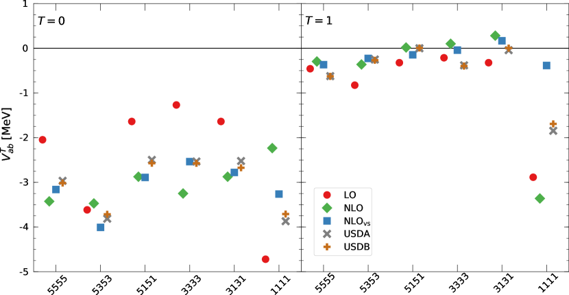
Figure 6: Monopole matrix elements of the different chiral shell-model interactions for mass number $A=18$. The left panel shows the monopole matrix elements for isospin $T=0$ and the right panel for $T=1$. The chiral shell-model interactions at LO, NLO, and NLO_vs are shown together with the monopole matrix elements of the USDA and USDB interactions from Ref. Brown and Richter (2006). The matrix elements are labeled by $2j_{a}\,2j_{b}\,2j_{a}\,2j_{b}$.

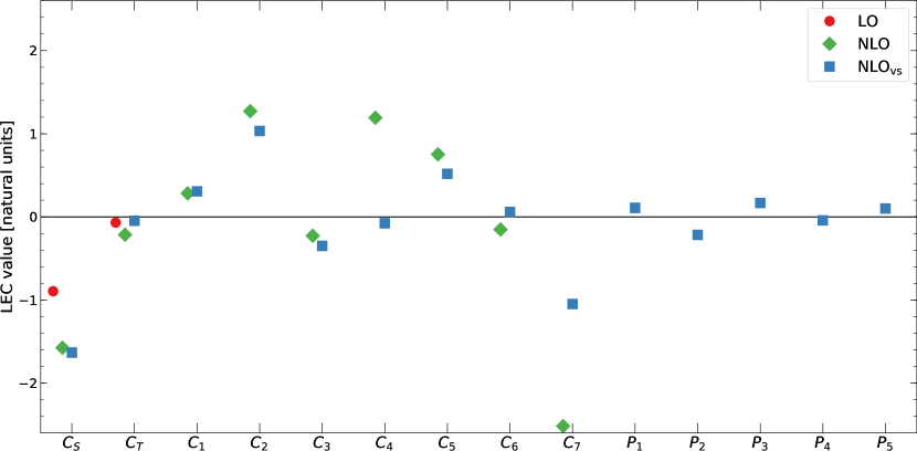
Figure 7: Fitted LECs at LO, NLO, and NLO_vs in natural units, which are obtained using Eqs. (10)–(12).

Figure 6 shows the monopole matrix elements of the chiral shell-model interactions at LO, NLO, and NLO_vs as well as those of the USDA and USDB interaction for $A=18$ (i.e., without applying the scaling with $\hbar\omega$). In the $T=0$ channel (left panel of Fig. 6), the monopole matrix elements at LO (except for 5353) deviate significantly from the other interactions, while at NLO and especially at NLO_vs they are similar to the monopole matrix elements of USDA/USDB. In general the change from NLO to NLO_vs is small except for the higher lying 1111 and 3333 orbitals. For the $T=1$ channel (right panel of Fig. 6), the changes from LO to NLO are significantly smaller, and there are only notable deviations from USDA/USDB for the 1111 monopole matrix element. The latter was also observed in microscopic calculations of valence-space Hamiltonians Otsuka et al. (2010a).

The resulting LECs at different orders are shown in Fig. 7. To express them in natural units (see, e.g., Ref. Epelbaum et al. (2005)), we multiply the LO and NLO LECs by

$$C_{\text{LO}}[\text{nat. units}] =C_{\text{LO}}\cdot F_{\pi}^{2}\,,$$ (10)

$$C_{\text{NLO}}[\text{nat. units}] =C_{\text{NLO}}\cdot\left(F_{\pi}\Lambda\right)^{2}\,,$$ (11)

$$P_{i}[\text{nat. units}] =P_{i}\cdot\left(F_{\pi}\Lambda\right)^{2}\,,$$ (12)

with $\Lambda=\Lambda_{\text{HO}}=375$ MeV and pion decay constant $F_{\pi}=92.4$ MeV. As shown in Fig. 7, all fitted LECs at all orders come out to be natural, or are very small in some cases. Wigner symmetry given by $C_{S}\gg C_{T}$ is also fulfilled by our interactions. Note that neither naturalness nor Wigner symmetry was imposed as a constraint on the fit. The LECs of the new CM-dependent operators are given by $P_{1-5}$ in Fig. 7. We find that all $P_{i}$ are similar in magnitude. Finally, the changes from LO to NLO and NLO_vs are also systematic for the LECs, with larger changes from NLO to NLO_vs mainly for $C_{4}$ and $C_{7}$.

IV Results

After a discussion of our fits and the overview of the comparison to experiment and to USD-type interactions in the previous section, we next present a more detailed picture of the quality of the chiral shell-model interactions. In most cases the experimental data shown are from the atomic mass evaluation Wang et al. (2012) for the ground-state energies and from Ref. nnd for excitation energies, otherwise the experimental reference is given explicitly. Moreover, experimental states included in the fit are shown in gray, and in red for predictions. We also provide the TBMEs and SPEs of the NLO_vs interaction in App. C.

IV.1 Uncertainty estimates

The EFT enables estimates of the theoretical uncertainty due to the truncation of the chiral expansion. We explore these uncertainties here after the chiral shell-model interactions have been fit, but will explore the fits within the optimization in future work. The purpose of the present uncertainty study is to obtain a feeling for these in the context of the shell-model calculations. We emphasize that these theoretical uncertainties do not include the systematic uncertainties from the shell-model basis or from possible states that have a small overlap with $sd$-shell configurations.

For the ground-state energies, we directly apply the chiral EFT uncertainty estimate from Ref. Epelbaum et al. (2015) and show the resulting uncertainties in Fig. 8. These are obtained at LO and NLO using

$$\Delta E_{\text{LO}}^{\text{gs}} =\left|E_{\text{LO}}^{\text{gs}}\right|Q^{2}\,,$$ (13)

$$\Delta E_{\text{NLO}}^{\text{gs}} =\max\bigl{(}\left|E_{\text{LO}}^{\text{gs}}\right|Q^{3},\,\left|E_{\text{LO}}^{\text{gs}}-E_{\text{NLO}}^{\text{gs}}\right|Q\bigr{)}\,,$$ (14)

where $Q=m_{\pi}/\Lambda_{b}$ with pion mass $m_{\pi}$, and we take $\Lambda_{b}=\Lambda_{\mathrm{HO}}=375$ MeV.

For excitation energies, the uncertainty estimates are more challenging. Because the excitation energies in medium-mass nuclei are small compared to the total energy scale, and because the LO interaction performs poorly in most nuclei (as expected with only two LECs), the theoretical uncertainty would be dominated by the large difference $\left|E_{\text{LO}}^{\text{ex}}-E_{\text{NLO}}^{\text{ex}}\right|$, if we were to follow the same prescription for the excited states as for the ground-state energies above. We therefore adopt the following to estimate the uncertainties for the excitation energies

$$\Delta E_{\text{LO}}^{\text{ex}} =\max\bigl{(}E^{\text{av}}_{\text{sd}},\,\left|E_{\text{LO}}^{\text{ex}}\right|\bigr{)}\,Q^{2}\,,$$ (15)

$$\Delta E_{\text{NLO}}^{\text{ex}} =\max\bigl{(}E^{\text{av}}_{\text{sd}},\,\left|E_{\text{NLO}}^{\text{ex}}\right|\bigr{)}\,Q^{3}\,,$$ (16)

where we have introduced the scale $E^{\text{av}}_{\text{sd}}=3$ MeV, which is taken to be approximately the average of the splittings between the $sd$-shell orbitals. This scale sets the natural scale for excitations in the $sd$ shell.

IV.2 Ground-state energies

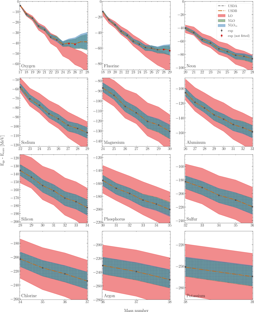
Figure 8: Ground-state energies from oxygen to potassium obtained from chiral shell-model interactions at LO, NLO, and NLO_vs. The energies are given with respect to the ¹⁶O core and are Coulomb corrected according to Tab. 1. The theoretical uncertainties are calculated with Eq. (13) at LO and with Eq. (14) at NLO. For comparison, we give the USDA and USDB results from Ref. Brown and Richter (2006). Experimental energies that are included in the fit are given by gray circles, while states that are not included are given by red squares for ^25,26O and ^28,29F.

In Fig. 8, we show the ground-state energies for the isotopic chains from oxygen to potassium based on the chiral shell-model interactions at LO, NLO, and NLO_vs including the theoretical uncertainties as discussed above. For comparison, also the USDA and USDB energies are given. We find that all states that were included in the fit are reproduced at all orders within the EFT uncertainties. However, the LO interaction predicts too much binding for the neutron-rich oxygen and fluorine isotopes that were not included in the fit. As a result, the oxygen dripline is not reproduced, being at or beyond ²⁸O at LO, and also ²⁸F and ²⁹F are overbound with respect to experiment. Remarkably, already the NLO interaction correctly reproduces the oxygen dripline as well as the two fluorine isotopes, which were not included in the fit. Moreover, the NLO and NLO_vs interactions overlap in all cases and reproduce ground-state energies equally well.

IV.3 Spectra

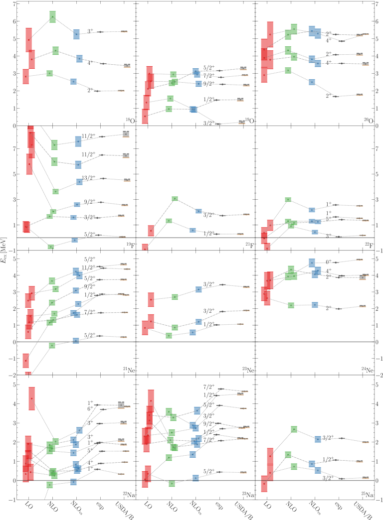
Figure 9: Excitation spectra of selected isotopes from oxygen to sodium. In each panel, results are shown for the chiral shell-model interactions at LO, NLO, and NLO_vs, in comparison to experiment and USDA/USDB results, where USDA (USDB) is visualized by a dashed gray (solid orange) line. The theoretical uncertainties are given by Eq. (15) at LO and by Eq. (16) at NLO. The same states are joined by dashed lines to guide the eye. The angular momentum labels are printed next to the experimental states. Isotope labels are given in the lower right corner.

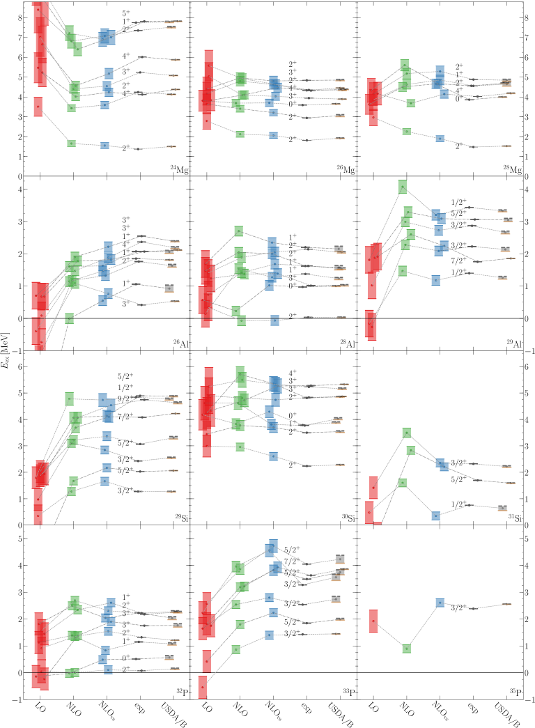
Figure 10: Excitation spectra of selected isotopes from magnesium to phosphorus. For details see the caption of Fig. 9.

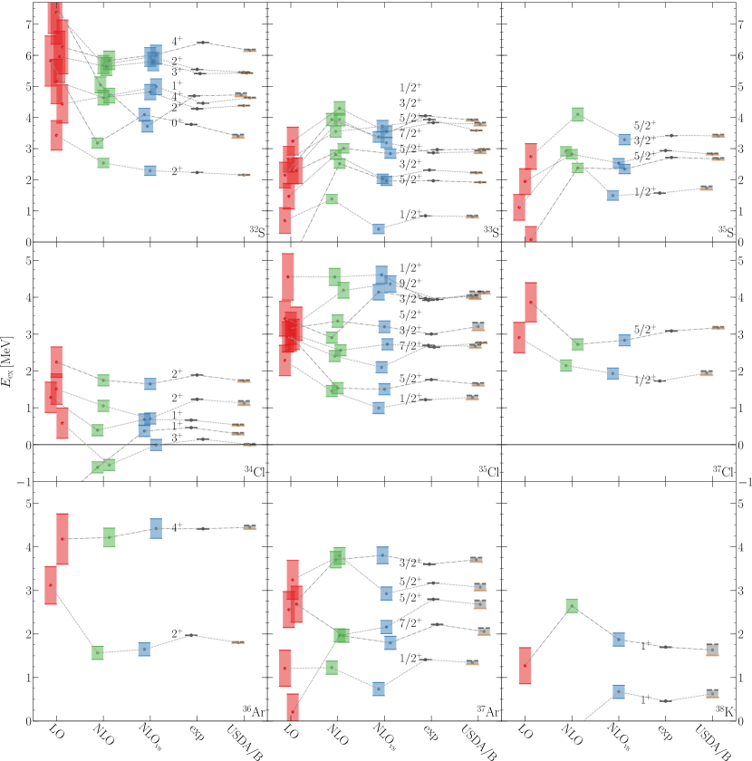
Figure 11: Excitation spectra of selected isotopes from sulfur to potassium. For details see the caption of Fig. 9.

In Figs. 9–11, we present our results for the spectra of excited states. These cover the $sd$ shell for representative cases of nuclei regarding the fits. In each panel, results are given for the chiral shell-model interactions at LO, NLO, and NLO_vs including the theoretical uncertainties, in comparison to experiment and the USDA/USDB interactions. First, in Fig. 9, we show results for oxygen, fluorine, neon, and sodium isotopes. For the oxygen spectra (first row), the excitation energies generally change weakly from LO to NLO to NLO_vs. From LO to NLO, the excitation energy usually increases, and the NLO_vs results generally lead to an improvement. In fluorine (second row), the NLO interaction already shows a clear improvement from the LO result, but overshoots the experimental value somewhat, where again then at NLO_vs the spectra are in good agreement with experiment. For the neon spectra (third row), most states show a continuous improvement from LO to NLO to NLO_vs. Moreover, by including the CM-dependent operators, the correct ground-state can be reproduced in ²¹Ne. For the sodium isotopes (fourth row), we show the two outliers ²²Na and ²³Na, which we already pointed to in the discussion of Fig. 3. In both of them we see that our interactions at NLO and NLO_vs lead to too low energies, and also that there is nearly no improvement from NLO to NLO_vs. However, ²⁵Na shows again a similar behavior as the fluorine isotopes.

In Fig. 10, we show results for magnesium, aluminum, silicon, and phosphorus isotopes. We generally find similar order-by-order behaviors described above, with an overall improvement going to NLO_vs. We note in particular the improvement for ²⁶Al, ³¹Si, and ³⁵P, as well as the correct reproduction of the ³²P ground state when the CM-dependent operators are included. In Fig. 11, we show results for the remaining sulfur, chlorine, argon, and potassium isotopes, which exhibit similar order-by-order trends as well. Another outlier here is the first excited state of ³⁷Ar, which is well reproduced by the LO and NLO interactions, but at slightly too low energy with the NLO_vs interaction. However, besides this first excited state, most of the remaining states improve with the NLO_vs interaction.

Finally, we need to comment on the theoretical uncertainties for the excited states. While the behavior of the uncertainties may not be unreasonable, the adopted prescription for the uncertainties of excitation energies is not fully satisfactory, in particular regarding the LO to NLO behavior which is not overlapping in many cases. Future work is needed here, with, e.g., a Bayesian analysis Furnstahl et al. (2015) of the order-by-order behavior of the results leading to improved estimates of the theoretical uncertainties.

IV.4 Predictions

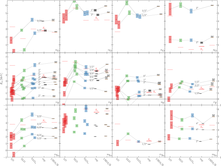
Figure 12: Predictions of excited states in oxygen, fluorine, and neon isotopes. For details on the labelling see the caption of Fig. 9. In addition to the ENSDF nnd spectra, we compare our results to experimental data in ²³O Elekes et al. (2007); Schiller et al. (2007), ²⁶O Kondo et al. (2016), ²⁴F Cáceres et al. (2015), and ^25,26F Vajta et al. (2014); Vandebrouck et al. (2017). Moreover, to emphasize the effects of the continuum, not included in our calculation, we give the calculated and experimental neutron separation energy $S_{n}$ as horizontal dashed line (see text).

After the promising prediction of the oxygen dripline at NLO and NLO_vs observed above, we also study the predictions for excited states of neutron-rich nuclei beyond the fitted data set. We focus on the spectra of neutron-rich oxygen, fluorine, and neon isotopes, which are plotted in Fig. 12. Only the first excited state in ²⁶Ne was included in the fit. All remaining states are predictions of the chiral shell-model interactions. Because our calculations do not include the continuum, we emphasize this by showing the neutron separation energy $S_{n}$ in Fig. 12. For states close to or above $S_{n}$, the explicit inclusion of the continuum will lead to changes, which are often of the order of few hundred keV unless this is further resonantly enhanced.

In comparison to measured states, the chiral shell-model interactions at NLO_vs again lead to the best overall agreement, and there is generally an improvement in going from LO to NLO to NLO_vs. For the oxygen isotopes this is especially visible in ^23,24O. Moreover, all our interactions reproduce the first 2⁺ energy in ²⁶O recently measured at RIKEN Kondo et al. (2016). This state is especially impressive, since neither the ground-state energy, nor the excitation energy was used in our dataset, and the order-by-order behavior is very stable. The agreement of our chiral shell-model interaction predictions at NLO_vs is also very good for the fluorine isotopes, especially for the low-lying states known, and for all neon isotopes shown.

V Summary and outlook

We have developed chiral shell-model interactions in the $sd$ shell, by fitting the LECs of chiral EFT operators at LO and NLO directly to 441 ground- and excited-state energies. In addition to the free-space contact interactions and pion exchanges, this includes novel CM-dependent operators that arise due to the breaking of Galilean invariance in the presence of the core.

The shell-model fits lead to a systematic improvement from LO to NLO and NLO_vs and resulted in natural LECs at all orders. The RMS derivation of the fits improved from 1.8 MeV at LO to 0.7 MeV at NLO and 0.5 MeV at NLO_vs. The latter includes five novel operators that depend on the two-body CM momentum, so that the total number of LECs at NLO_vs is 14. In comparison to USD-type interactions, the RMS deviation is about 200 keV higher, but shows a similar rapid improvement with the number of LECs. Moreover, the monopole matrix elements are similar to the successful USDA/USDB interactions at NLO and NLO_vs. Therefore, we conclude that the chiral EFT operators efficiently capture the relevant physics at low energies. The EFT expansion enabled us to provide theoretical uncertainties, which seem very systematic for ground-state energies, but require further developments for the excitation energies.

We have found a very good reproduction of experimental ground-state energies at all orders, and a striking improvement in the reproduction of excitation energies from LO to NLO and NLO_vs. Moreover, the overall systematic improvement from NLO to NLO_vs and the fact that some states could only be reproduced, e.g., with the correct ground-state spin at NLO_vs, confirms the importance of the inclusion of the new CM-dependent operators for chiral shell-model interactions. The developed interactions show promising predictions for neutron-rich isotopes beyond the fitted data set. In addition to the correct reproduction of the oxygen dripline already at NLO, the excited states in neutron-rich oxygen, fluorine, and neon isotopes, which were not included in the fit, are predicted very well at NLO_vs.

Besides improving the way theoretical uncertainties can be assessed for excited states, future work includes going to higher order, which will include also three-nucleon interactions, and the exploration of consistent electroweak transition based on chiral EFT operators. Moreover, for valence-space Hamiltonians beyond a single major shell, where phenomenological interactions involve ad hoc reductions of the cross-shell matrix elements, the strategy presented here could provide interesting new interactions. This is especially important for exotic nuclei and for heavier nuclei, including key nuclei for neutrinoless double-beta decay.

Appendix A Partial-wave decomposition

A.1 Free-space contact interactions

In the following, we give the partial-wave decomposition of the LO and NLO contact interactions, where

$$\braket{\textbf{p}}{\bm{\mathrm{V}}_{C_{i}}}{\textbf{p}^{\prime}}\longrightarrow C_{i}\,V_{C_{i}}^{ll^{\prime}sj}(p,p^{\prime})\,,$$ (17)

when projected on a given partial wave. The free-space contact interactions lead to

$$V_{C_{S}}^{ll^{\prime}sj}(p,p^{\prime})=4\pi\delta_{ll^{\prime}}\delta_{l0}\,,$$ (18)

$$V_{C_{T}}^{ll^{\prime}sj}(p,p^{\prime})=4\pi\delta_{ll^{\prime}}\delta_{l0}\bigl{(}2s(s+1)-3\bigr{)}\,,$$ (19)

$$V_{C_{1}}^{ll^{\prime}sj}(p,p^{\prime})=4\pi\delta_{ll^{\prime}}\Bigl{(}\delta_{l0}(p^{2}+p^{\prime 2})-\frac{2}{3}\delta_{l1}pp^{\prime}\Bigr{)}\,,$$ (20)

$$V_{C_{2}}^{ll^{\prime}sj}(p,p^{\prime})=\pi\delta_{ll^{\prime}}\Bigl{(}\delta_{l0}(p^{2}+p^{\prime 2})+\frac{2}{3}\delta_{l1}pp^{\prime}\Bigr{)}\,,$$ (21)

$$V_{C_{3}}^{ll^{\prime}sj}(p,p^{\prime})=\bigl{(}2s(s+1)-3\bigr{)}V_{C_{1}}^{ll^{\prime}sj}(p,p^{\prime})\,,$$ (22)

$$V_{C_{4}}^{ll^{\prime}sj}(p,p^{\prime})=\bigl{(}2s(s+1)-3\bigr{)}V_{C_{2}}^{ll^{\prime}sj}(p,p^{\prime})\,,$$ (23)

$$V_{C_{5}}^{ll^{\prime}sj}(p,p^{\prime})=\delta_{ll^{\prime}}\delta_{s1}\delta_{l1}\frac{2\pi}{3}\bigl{(}4-j(j+1)\bigr{)}pp^{\prime}\,,$$ (24)

$$V_{C_{6}}^{ll^{\prime}sj}(p,p^{\prime})=$$

$$24\pi\sum\limits_{a=0,2}(-1)^{s+j+l^{\prime}+a}\,\widehat{a}\,\widehat{s}^{\,2}\begin{Bmatrix}l&s&j\\ s&l^{\prime}&a\end{Bmatrix}\begin{Bmatrix}1&1&a\\ 1/2&1/2&s\\ 1/2&1/2&s\end{Bmatrix}$$

$$\times\left[C^{a0}_{1010}\left(p^{2}\delta_{la}\delta_{l^{\prime}0}+p^{\prime 2}\delta_{l0}\delta_{l^{\prime}a}\right)+\frac{2}{3}\widehat{a}\,pp^{\prime}\delta_{ll^{\prime}}\delta_{l1}\right]\,,$$ (25)

$$V_{C_{7}}^{ll^{\prime}sj}(p,p^{\prime})=$$

$$6\pi\sum\limits_{a=0,2}(-1)^{s+j+l^{\prime}+a}\,\widehat{a}\,\widehat{s}^{\,2}\begin{Bmatrix}l&s&j\\ s&l^{\prime}&a\end{Bmatrix}\begin{Bmatrix}1&1&a\\ 1/2&1/2&s\\ 1/2&1/2&s\end{Bmatrix}$$

$$\times\left[C^{a0}_{1010}\left(p^{2}\delta_{la}\delta_{l^{\prime}0}+p^{\prime 2}\delta_{l0}\delta_{l^{\prime}a}\right)-\frac{2}{3}\widehat{a}\,pp^{\prime}\delta_{ll^{\prime}}\delta_{l1}\right]\,.$$ (26)

where $\widehat{a}=\sqrt{2a+1}$, $C^{lm}_{l_{1}m_{1}l_{2}m_{2}}$ is a Clebsch-Gordan coefficient, and $\left\{\cdots\right\}$ are Wigner 6j- and 9j-symbols.

A.2 Center-of-mass–dependent operators

Similar to the free-space contact interactions, we give the partial-wave decomposition of the CM-dependent operators with

$$\braket{\textbf{p},\textbf{P}}{\bm{\mathrm{V}}_{P_{i}}}{\textbf{p}^{\prime},\textbf{P}^{\prime}}\longrightarrow\frac{\delta(P-P^{\prime})}{PP^{\prime}}P_{i}\braket{\text{rel,cm}}{V^{J}_{P_{i}}}{\text{rel${}^{\prime}$,cm${}^{\prime}$}}\,,$$

where we use the short-hand notation

$$\braket{\text{rel,cm}}{V^{J}}{\text{rel${}^{\prime}$,cm${}^{\prime}$}}=\braket{pP[(ls)jL]J}{V}{p^{\prime}P[(l^{\prime}s^{\prime})j^{\prime}L^{\prime}]J}\,,$$ (27)

which is diagonal in $P$, since the total momentum is conserved, and diagonal in total angular momentum ${\bf J}={\bf j}+{\bf L}$, but not diagonal in $s,s^{\prime}$ or $j,j^{\prime}$. With this, the partial-wave decomposition reads

$$\braket{\text{rel,cm}}{V^{J}_{P_{1}}}{\text{rel${}^{\prime}$,cm${}^{\prime}$}}=4\pi P^{2}\delta_{ss^{\prime}}\delta_{ll^{\prime}}\delta_{l0}\delta_{jj^{\prime}}\delta_{js}\delta_{LL^{\prime}}\,,$$ (28)

$$\braket{\text{rel,cm}}{V^{J}_{P_{2}}}{\text{rel${}^{\prime}$,cm${}^{\prime}$}}=4\pi P^{2}\delta_{ss^{\prime}}\delta_{ll^{\prime}}\delta_{l0}\delta_{jj^{\prime}}\delta_{js}\delta_{LL^{\prime}}$$

$$\quad\times\bigl{(}2s(s+1)-3\bigr{)}\,,$$ (29)

$$\braket{\text{rel,cm}}{V^{J}_{P_{3}}}{\text{rel${}^{\prime}$,cm${}^{\prime}$}}=24\pi\sqrt{2}\,\delta_{s+s^{\prime},1}\,\widehat{j}\widehat{j^{\prime}}\widehat{L^{\prime}}$$

$$\quad\times C^{L0}_{L^{\prime}010}\begin{Bmatrix}j&L&J\\ L^{\prime}&j^{\prime}&1\end{Bmatrix}\begin{Bmatrix}1&1&1\\ l&s&j\\ l^{\prime}&s^{\prime}&j^{\prime}\end{Bmatrix}$$

$$\quad\times(-1)^{L+J+j^{\prime}+s^{\prime}+1}\left(\delta_{l1}\delta_{l^{\prime}0}p+\delta_{l0}\delta_{l^{\prime}1}p^{\prime}\right)P\,,$$ (30)

$$\braket{\text{rel,cm}}{V^{J}_{P_{4}}}{\text{rel${}^{\prime}$,cm${}^{\prime}$}}=12\pi\sqrt{2}\,\delta_{s+s^{\prime},1}\,\widehat{j}\widehat{j^{\prime}}\widehat{L^{\prime}}$$

$$\quad\times C^{L0}_{L^{\prime}010}\begin{Bmatrix}j&L&J\\ L^{\prime}&j^{\prime}&1\end{Bmatrix}\begin{Bmatrix}1&1&1\\ l&s&j\\ l^{\prime}&s^{\prime}&j^{\prime}\end{Bmatrix}$$

$$\quad\times(-1)^{L+J+j^{\prime}}\left(\delta_{l1}\delta_{l^{\prime}0}p-\delta_{l0}\delta_{l^{\prime}1}p^{\prime}\right)P\,,$$ (31)

and

$$\braket{\text{rel,cm}}{V^{J}_{P_{5}}}{\text{rel${}^{\prime}$,cm${}^{\prime}$}}=24\pi\delta_{ss^{\prime}}\delta_{ll^{\prime}}\delta_{l0}\delta_{jj^{\prime}}\widehat{L^{\prime}}\,\widehat{s}^{\,2}$$

$$\quad\times\sum\limits_{a=0,2}\widehat{a}\,C^{a0}_{1010}C^{L0}_{L^{\prime}0a0}\begin{Bmatrix}j&L&J\\ L^{\prime}&j&a\end{Bmatrix}\begin{Bmatrix}1&1&a\\ 1/2&1/2&s\\ 1/2&1/2&s\end{Bmatrix}$$

$$\quad\times(-1)^{L+J+j}P^{2}\,.$$ (32)

Appendix B Transformation to HO basis

To calculate the TBMEs, we first transform the partial-wave momentum-space matrix elements to the relative-CM HO basis

$$\braket{nN[(ls)jL]{J}}{V}{n^{\prime}N^{\prime}[(l^{\prime}s^{\prime})j^{\prime}L^{\prime}]{J}}$$

$$=\int dpp^{2}R_{nl}(p)\int dp^{\prime}p^{\prime 2}R_{n^{\prime}l^{\prime}}(p^{\prime})$$

$$\times\int dPP^{2}R_{NL}(P)R_{N^{\prime}L^{\prime}}(P)\braket{\text{rel,cm}}{V^{J}}{\text{rel${}^{\prime}$,cm${}^{\prime}$}}\,.$$ (33)

The relative-CM HO matrix elements are then transformed to the TBMEs using the Talmi-Moshinsky transformation. Including also the isospin part, this leads to

$$\braket{nN[(ls)jL]JT}{V}{n^{\prime}N^{\prime}[(l^{\prime}s^{\prime})j^{\prime}L^{\prime}]JT}\rightarrow$$

$$\braket{(n_{1}l_{1}j_{1})(n_{2}l_{2}j_{2})JT}{V}{(n^{\prime}_{1}l^{\prime}_{1}j^{\prime}_{1})(n^{\prime}_{2}l^{\prime}_{2}j^{\prime}_{2})JT}=$$

$$\Braket{n_{1}n_{2}\Bigl{[}(l_{1}\frac{1}{2})j_{1}(l_{2}\frac{1}{2})j_{2}\Bigr{]}JT}{V}{n^{\prime}_{1}n^{\prime}_{2}\Bigl{[}(l^{\prime}_{1}\frac{1}{2})j^{\prime}_{1}(l^{\prime}_{2}\frac{1}{2})j^{\prime}_{2}\Bigr{]}JT}.$$ (34)

To this end, we first recouple the two-body states to $\ket{n_{1}n_{2}[(l_{1}l_{2}){\Lambda}(\frac{1}{2}\frac{1}{2})s]J}$, with total orbital angular momentum ${\bm{\Lambda}}={\bf l}_{1}+{\bf l}_{2}$ or in terms of relative and CM angular momenta ${\bm{\Lambda}}={\bf L}+{\bf l}$, and then to two-body states $\ket{Nn[(Ll)\Lambda s]J}$, which can be recoupled to the desired relative-CM states $\ket{nN[(ls)jL]J}$. Combining this, we have for antisymmetrized, normalized two-body states

$$\Ket{n_{1}n_{2}\Bigl{[}(l_{1}\frac{1}{2})j_{1}(l_{2}\frac{1}{2})j_{2}\Bigr{]}JT}=\sum_{\Lambda s}\widehat{\Lambda}\widehat{s}\,\widehat{j_{1}}\widehat{j_{2}}\begin{Bmatrix}l_{1}&l_{2}&\Lambda\\ 1/2&1/2&s\\ j_{1}&j_{2}&J\end{Bmatrix}$$

$$\times\sum_{nlNL}\braket{Nn(Ll)\Lambda}{n_{1}n_{2}(l_{1}l_{2})\Lambda}_{d=1}$$

$$\times\sum_{j}(-1)^{l+s+j}\,\widehat{\Lambda}\widehat{j}\begin{Bmatrix}L&l&\Lambda\\ s&J&j\end{Bmatrix}{\mathcal{F}}\ket{nN[(ls)jL]JT}\,,$$ (35)

where ${\mathcal{F}}=(1-(-1)^{l+s+T})/\sqrt{2(1+\delta_{n_{1}n_{2}}\delta_{l_{1}l_{2}}\delta_{j_{1}j_{2}})}$ takes into account the normalization and antisymmetrization of the two-body states, and $\braket{Nn(Ll)\Lambda}{n_{1}n_{2}(l_{1}l_{2})\Lambda}_{d=1}$ is the Talmi-Moshinsky bracket in the conventions of Ref. Kamuntavičius et al. (2001). Note that for calculating the TMBEs the sum is over all $s,s^{\prime}$, $j,j^{\prime}$, $N,N^{\prime}$, and $L,L^{\prime}$, contrary to the case for free-space interactions when these are diagonal.

Appendix C Two-body matrix elements

For completeness, we list the TBMEs of the NLO_vs interaction in Table 3. The corresponding SPEs are $\varepsilon_{0d_{5/2}}=-4.14308\,\mathrm{MeV}$, $\varepsilon_{1s_{1/2}}=-3.27235\,\mathrm{MeV}$, and $\varepsilon_{0d_{3/2}}=0.94172\,\mathrm{MeV}$, taken from the spectrum of ¹⁷O.

Table 3: Two-body matrix elements for the NLO_vs interaction for a given isospin $T$ and total angular momentum $J$. The single-particle orbits are labelled by $2j_{a}\,2j_{b}\,2j_{c}\,2j_{d}$.

orbitals	$T$	$J=0$	$J=1$	$J=2$	$J=3$	$J=4$	$J=5$
$5555$	0	–	$-2.962356$	–	$-1.348477$	–	$-4.366727$
	1	$-1.561786$	–	$-0.591304$	–	$-0.109698$	–
$5553$	0	–	2.203146	–	1.185351	–	–
	1	–	–	$-0.782881$	–	$-0.958506$	–
$5551$	0	–	–	–	$-1.671394$	–	–
	1	–	–	$-0.744657$	–	–	–
$5533$	0	–	0.893444	–	0.528466	–	–
	1	$-5.086935$	–	$-1.053896$	–	–	–
$5531$	0	–	0.568667	–	–	–	–
	1	–	–	0.908236	–	–	–
$5511$	0	–	$-0.106744$	–	–	–	–
	1	$-1.483464$	–	–	–	–	–
$5353$	0	–	$-5.783199$	$-4.103275$	$-2.055604$	$-4.881107$	–
	1	–	0.302405	0.624787	$-0.239897$	$-0.866801$	–
$5351$	0	–	–	$-1.513283$	1.363597	–	–
	1	–	–	$-0.029187$	0.039135	–	–
$5333$	0	–	$-1.067963$	–	1.696282	–	–
	1	–	–	$-0.728416$	–	–	–
$5331$	0	–	1.558985	$-2.312917$	–	–	–
	1	–	$0.083957$	0.922578	–	–	–
$5311$	0	–	1.400007	–	–	–	–
	1	–	–	–	–	–	–
$5151$	0	–	–	$-1.943009$	$-3.565486$	–	–
	1	–	–	$-0.654884$	0.217367	–	–
$5133$	0	–	–	–	0.001177	–	–
	1	–	–	$-0.684786$	–	–	–
$5131$	0	–	–	$-1.984955$	–	–	–
	1	–	–	1.534945	–	–	–
$3333$	0	–	$-1.635266$	–	$-2.921386$	–	–
	1	$-0.014457$	–	$-0.046811$	–	–	–
$3331$	0	–	$-0.996922$	–	–	–	–
	1	–	–	0.179512	–	–	–
$3311$	0	–	$-0.309804$	–	–	–	–
	1	$-1.585586$	–	–	–	–	–
$3131$	0	–	$-3.190265$	$-2.531388$	–	–	–
	1	–	0.054273	0.236452	–	–	–
$3111$	0	–	0.139808	–	–	–	–
	1	–	–	–	–	–	–
$1111$	0	–	$-3.262572$	–	–	–	–
	1	$-0.385534$	–	–	–	–	–

References

- Brown (2001) B. A. Brown, Prog. Part. Nucl. Phys. 47, 517 (2001).
- Caurier et al. (2005) E. Caurier, G. Martinez-Pinedo, F. Nowacki, A. Poves, and A. P. Zuker, Rev. Mod. Phys. 77, 427 (2005).
- Coraggio et al. (2009) L. Coraggio, A. Covello, A. Gargano, N. Itaco, and T. T. S. Kuo, Prog. Part. Nucl. Phys. 62, 135 (2009).
- Brown and Richter (2006) B. A. Brown and W. A. Richter, Phys. Rev. C 74, 034315 (2006).
- Hjorth-Jensen et al. (1995) M. Hjorth-Jensen, T. T. S. Kuo, and E. Osnes, Phys. Rep. 261, 125 (1995).
- Holt et al. (2014) J. D. Holt, J. Menéndez, J. Simonis, and A. Schwenk, Phys. Rev. C 90, 024312 (2014).
- Simonis et al. (2016) J. Simonis, K. Hebeler, J. D. Holt, J. Menéndez, and A. Schwenk, Phys. Rev. C 93, 011302(R) (2016).
- Dikmen et al. (2015) E. Dikmen, A. F. Lisetski, B. R. Barrett, P. Maris, A. M. Shirokov, and J. P. Vary, Phys. Rev. C 91, 064301 (2015).
- Barrett et al. (2013) B. R. Barrett, P. Navrátil, and J. P. Vary, Prog. Part. Nucl. Phys. 69, 131 (2013).
- Jansen et al. (2014) G. R. Jansen, J. Engel, G. Hagen, P. Navrátil, and A. Signoracci, Phys. Rev. Lett. 113, 142502 (2014).
- Jansen et al. (2016) G. R. Jansen, A. Signoracci, G. Hagen, and P. Navrátil, Phys. Rev. C 94, 011301(R) (2016).
- Hagen et al. (2014) G. Hagen, T. Papenbrock, M. Hjorth-Jensen, and D. J. Dean, Rep. Prog. Phys. 77, 096302 (2014).
- Tsukiyama et al. (2012) K. Tsukiyama, S. K. Bogner, and A. Schwenk, Phys. Rev. C 85, 061304(R) (2012).
- Bogner et al. (2014) S. K. Bogner, H. Hergert, J. D. Holt, A. Schwenk, S. Binder, A. Calci, J. Langhammer, and R. Roth, Phys. Rev. Lett. 113, 142501 (2014).
- Stroberg et al. (2017) S. R. Stroberg, A. Calci, H. Hergert, J. D. Holt, S. K. Bogner, R. Roth, and A. Schwenk, Phys. Rev. Lett. 118, 032502 (2017).
- Hergert et al. (2016) H. Hergert, S. K. Bogner, T. D. Morris, A. Schwenk, and K. Tsukiyama, Phys. Rept. 621, 165 (2016).
- Epelbaum et al. (2009) E. Epelbaum, H.-W. Hammer, and U.-G. Meißner, Rev. Mod. Phys. 81, 1773 (2009).
- Machleidt and Entem (2011) R. Machleidt and D. R. Entem, Phys. Rep. 503, 1 (2011).
- Weinberg (1990) S. Weinberg, Phys. Lett. B 251, 288 (1990).
- Weinberg (1991) S. Weinberg, Nucl. Phys. B 363, 3 (1991).
- Schwenk and Friman (2004) A. Schwenk and B. Friman, Phys. Rev. Lett. 92, 082501 (2004).
- Conze et al. (1973) M. Conze, H. Feldmeier, and P. Manakos, Phys. Lett. B 43, 101 (1973).
- Huth et al. (2017) L. Huth, I. Tews, J. E. Lynn, and A. Schwenk, Phys. Rev. C 96, 054003 (2017).
- König et al. (2014) S. König, S. K. Bogner, R. J. Furnstahl, S. N. More, and T. Papenbrock, Phys. Rev. C 90, 064007 (2014).
- Caurier and Nowacki (1999) E. Caurier and F. Nowacki, Acta Phys. Polon. B 30, 705 (1999).
- (26) T. Munson, J. Sarich, S. M. Wild, S. Benson, and J. Curfman McInne, Technical Memorandum ANL/MCS-TM-322, Argonne National Laboratory, Argonne, Illinois (2012), see http://www.mcs.anl.gov/tao.
- Wild et al. (2015) S. M. Wild, J. Sarich, and N. Schunck, J. Phys. G 42, 034031 (2015).
- Nelder and Mead (1965) J. A. Nelder and R. Mead, Comput. J. 7, 308 (1965).
- Otsuka et al. (2010a) T. Otsuka, T. Suzuki, J. D. Holt, A. Schwenk, and Y. Akaishi, Phys. Rev. Lett. 105, 032501 (2010a).
- Otsuka et al. (2010b) T. Otsuka, T. Suzuki, M. Honma, Y. Utsuno, N. Tsunoda, K. Tsukiyama, and M. Hjorth-Jensen, Phys. Rev. Lett. 104, 012501 (2010b).
- Holt et al. (2012) J. D. Holt, T. Otsuka, A. Schwenk, and T. Suzuki, J. Phys. G: Nucl. Part. Phys. 39, 085111 (2012).
- Epelbaum et al. (2005) E. Epelbaum, W. Glöckle, and U.-G. Meißner, Nucl. Phys. A 747, 362 (2005).
- Wang et al. (2012) M. Wang, G. Audi, A. H. Wapstra, F. G. Kondev, M. MacCormick, X. Xu, and B. Pfeiffer, Chin. Phys. C 36, 1603 (2012).
- (34) http://www.nndc.bnl.gov/ensdf/.
- Epelbaum et al. (2015) E. Epelbaum, H. Krebs, and U.-G. Meißner, Eur. Phys. J. A 51, 53 (2015).
- Furnstahl et al. (2015) R. J. Furnstahl, N. Klco, D. R. Phillips, and S. Wesolowski, Phys. Rev. C 92, 024005 (2015).
- Elekes et al. (2007) Z. Elekes, Z. Dombrádi, N. Aoi, S. Bishop, Z. Fülöp, J. Gibelin, T. Gomi, Y. Hashimoto, N. Imai, N. Iwasa, et al., Phys. Rev. Lett. 98, 102502 (2007).
- Schiller et al. (2007) A. Schiller, N. Frank, T. Baumann, D. Bazin, B. A. Brown, J. Brown, P. A. DeYoung, J. E. Finck, A. Gade, J. Hinnefeld, et al., Phys. Rev. Lett. 99, 112501 (2007).
- Kondo et al. (2016) Y. Kondo, T. Nakamura, R. Tanaka, R. Minakata, S. Ogoshi, N. A. Orr, N. L. Achouri, T. Aumann, H. Baba, F. Delaunay, et al., Phys. Rev. Lett. 116, 102503 (2016).
- Cáceres et al. (2015) L. Cáceres, A. Lepailleur, O. Sorlin, M. Stanoiu, D. Sohler, Z. Dombrádi, S. K. Bogner, B. A. Brown, H. Hergert, J. D. Holt, et al., Phys. Rev. C 92, 014327 (2015).
- Vajta et al. (2014) Z. Vajta, M. Stanoiu, D. Sohler, G. R. Jansen, F. Azaiez, Z. Dombrádi, O. Sorlin, B. A. Brown, M. Belleguic, C. Borcea, et al., Phys. Rev. C 89, 054323 (2014).
- Vandebrouck et al. (2017) M. Vandebrouck, A. Lepailleur, O. Sorlin, T. Aumann, C. Caesar, M. Holl, V. Panin, F. Wamers, S. R. Stroberg, J. D. Holt, et al., Phys. Rev. C 96, 054305 (2017).
- Kamuntavičius et al. (2001) G. P. Kamuntavičius, R. K. Kalinauskas, B. R. Barrett, S. Mickevičius, and D. Germanas, Nucl. Phys. A 695, 191 (2001).