AN EFFICIENT DEEP CONVOLUTIONAL LAPLACIAN PYRAMID ARCHITECTURE FOR CS RECONSTRUCTION AT LOW SAMPLING RATIOS
Abstract
The compressed sensing (CS) has been successfully applied to image compression in the past few years as most image signals are sparse in a certain domain. Several CS reconstruction models have been proposed and obtained superior performance. However, these methods suffer from blocking artifacts or ringing effects at low sampling ratios in most cases. To address this problem, we propose a deep convolutional Laplacian Pyramid Compressed Sensing Network (LapCSNet) for CS, which consists of a sampling sub-network and a reconstruction sub-network. In the sampling sub-network, we utilize a convolutional layer to mimic the sampling operator. In contrast to the fixed sampling matrices used in traditional CS methods, the filters used in our convolutional layer are jointly optimized with the reconstruction sub-network. In the reconstruction sub-network, two branches are designed to reconstruct multi-scale residual images and muti-scale target images progressively using a Laplacian pyramid architecture. The proposed LapCSNet not only integrates multi-scale information to achieve better performance but also reduces computational cost dramatically. Experimental results on benchmark datasets demonstrate that the proposed method is capable of reconstructing more details and sharper edges against the state-of-the-arts methods.
Index Terms— Compressed sensing, deep networks, image compression, laplacian pyramid, residual learning
1 Introduction
The compressed sensing theory [1, 2] shows that if a signal is sparse in a certain domain , it can be accurately recovered from a small number of random linear measurements less than that of Nyquist sampling theorem. Mathematically, the measurements are obtained by the following linear transformation
| (1) |
where is the signal, is known as the measurement vector, is the measurement matrix and denotes noise. If , reconstructing from is generally ill-posed, which is one of the most challenging issues in compressed sensing.
To design an efficient CS reconstruction algorithm, many methods have been proposed, which can be generally divided into two categories: traditional optimization-based methods and recent DNN-based methods.
In the optimization-based reconstruction methods, given the linear projections , the original image can be reconstructed by solving the following convex optimization problem [1, 2]:
| (2) |
To solve this convex problem, many algorithms have been proposed [4, 5, 6]. However, these algorithms suffer from uncertain reconstruction qualities and high computation cost, which inevitably limit their applications in practice.
Recently, some DNN-based algorithms have been proposed for image CS reconstruction. In [7], Mousavi et al. propose to utilize a stacked denoising autoencoder (SDA) to reconstruct original images from their measurements. A series of convolutional layers are adopted in [8, 9, 3] for image reconstruction. Despite their impressive results, massive block artifacts and ringing effects are delivered at low sampling ratios.
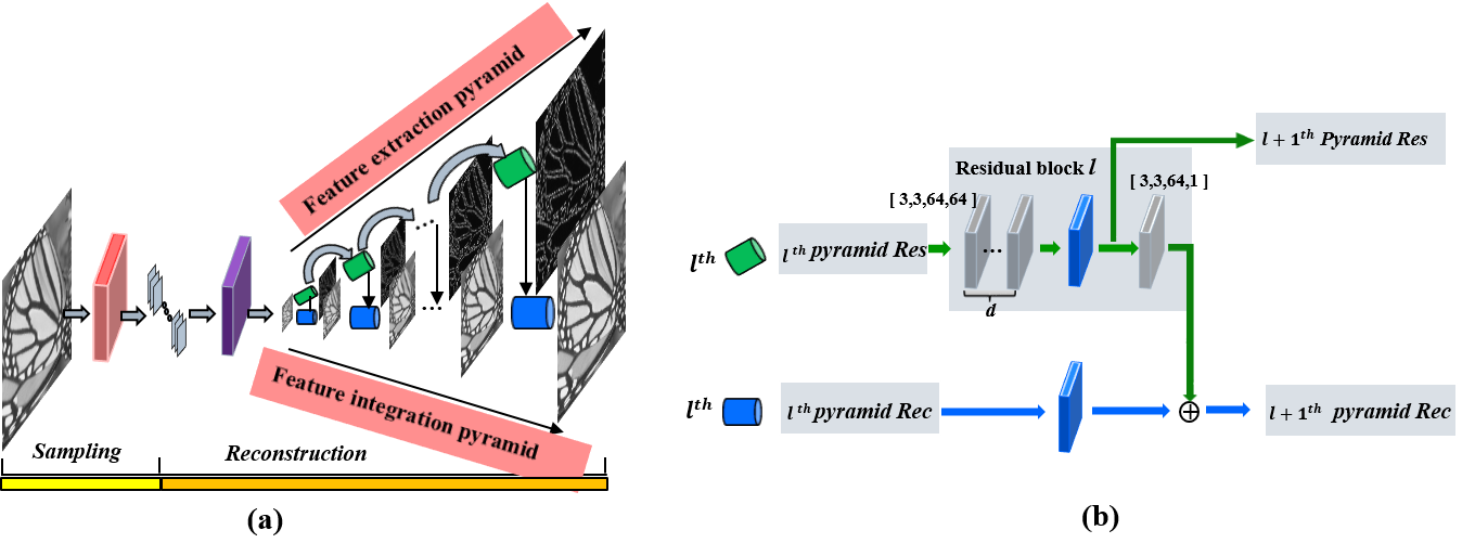
To overcome the shortcomings of the aforementioned methods, we propose a Laplacian Pyramid based deep architecture for CS reconstruction. Our network contains two sub-networks: sampling sub-network and reconstruction sub-network. In the sampling sub-network, a convolutional layer with the kernel size of ( is the size of current block) is utilized to mimic the sampling process. In the reconstruction sub-network, we use two branches to reconstruct multi-scale residual features and multi-scale target images progressively through Laplacian pyramid architectures. Besides, the second branch integrates multi-scale information from the first branch to preserve finer textures. The sampling sub-network and reconstruction sub-network are optimized jointly with the robust Charbonnier loss [10].
2 PROPOSED METHOD
In this section, we describe the methodology of the proposed LapCSNet including the sampling sub-network and the reconstruction sub-network as well as the loss function.

OriginalPSNRSSIM
HM12.590.1586
Cos19.130.5987
GSR21.010.6083
ReconNet19.960.5726

BCSNet23.460.6508
CSNet25.730.7209

Ours26.680.7588

OriginalPSNRSSIM
HM18.850.6909
Cos17.660.6546
GSR20.740.6832
ReconNet20.000.6706
BCSNet22.570.7531

CSNet24.900.8098
Ours25.570.8351
2.1 Sampling Sub-network
In traditional block-based compressed sensing (BCS), each row of the sampling matrix can be considered as a filter. Therefore, the sampling process can be mimicked using a convolutional layer [9, 3]. In our model, we use a convolutional layer with filters and set stride as for non-overlapping blocks. Specifically, given an image with size , there are a total of non-overlapping blocks with size (). The dimensions of measurements for each block is , Therefore, the dimensions of measurements for the current image is . Traditional sampling matrices are fixed for various reconstruction algorithms. The proposed DNN-based sampling matrices are learned jointly with the reconstruction sub-network from large amounts of data.
2.2 Reconstruction Sub-network
For the CS reconstruction, several DNN-based models have been proposed [8, 9]. These methods are implemented for each block, which ignore the relationship between blocks and therefore results in serious blocking artifacts in most cases. To solve this problem, we adopt a “reshape+concat” layer [3] to concatenate all blocks to obtain initial reconstruction, which is then refined to obtain superior reconstruction.
Initial reconstruction Given the compressed measurements, the initial reconstruction block can be obtained by
| (3) |
where is the measurement of the current block and is the scale factor for current block. is a matrix. In the aforementioned methods without scaling (), is difficult to be accurate calculated. By introducing the pyramid structure, a small block is first reconstructed in our method. Let and . The optimal scale factor is obtained as
| (4) |
where is used to return the maximal element of a set. Therefore, in our model. The convolution output of an image block in the sampling sub-network is a vector, so the size of the convolution filter in the initial reconstruction layer is . We use stride convolution to reconstruct each block. Since a smaller version of the target block is reconstructed, convolution filters of size are used. However, the reconstructed outputs of each block is still a vector. To obtain the initial reconstructed image, a “reshape+concat” layer is adopted. This layer first reshapes each reconstructed vector into a block, then concatenates all the blocks to get the reconstructed image. From Eq. (4), we can get that when , we can not obtain the smaller version of the target image. In this case, we only use this model for CS reconstruction at low sampling ratios.
Further reconstruction CSNet [3] has only 5 layers for CS reconstruction, which results in poor performance at low sampling ratios. Deep networks and elaborated architectures are essential for accurate reconstruction while increasing computational complexity due to the unenlightened superposition of convolutional layers. Our further reconstruction network takes the output of initial reconstruction as input and progressively predicts residual images at a total of levels where is the scale factor from Eq. 4. Moreover, our reconstruction model has two branches: residual feature extraction [11] and feature integration.
Multi-scale residual feature extraction: There is a one-to-one correspondence between reconstruction levels and residual blocks (shown in Fig. 1). In level , the corresponding residual block consists of convolutional layers and one transposed convolutional layer [12] to upsample the extracted features by a scale of . The output of each transposed convolutional layer is connected to two different layers: a convolutional layer for reconstructing a residual image for level ; a convolutional layer for extracting features in next level . Note that the residual feature at lower levels are shared with higher levels and thus can increase the non-linearity of the network to reconstruct the target image. Moreover, the hierarchical architecture is used for the CS feature extraction, which can preserve more details.
Multi-scale feature integration: In level , the input image is up-sampled by a scale of 2 using a transposed convolutional layer [12]. The upsampled image is then combined with the predicted residual images from the residual feature extraction branch. Then, the output in this level is fed into the next reconstruction module of level +1. This integration architecture fuses the the multi-scale residual branch and corresponding reconstruction branch efficiently. In addition, most of convolution operation are executed on the smaller version of the target image, which indicates our model is more efficient than the existing models with the same depth.
| Alg. | sampling ratio 0.01 | sampling ratio 0.02 | sampling ratio 0.1 | Avg. |
| TV [5] | 16.310.410122.48– | 17.940.443917.56– | 18.330.59216.93– | 17.530.482015.66– |
| MH [13] | 12.430.199984.32– | 20.620.538178.59– | 28.570.821169.27– | 20.540.519777.39– |
| Cos [14] | 17.420.412230487.56– | 18.460.482727453.49– | 29.550.85226433.25– | 21.810.582421454.65– |
| GSR [6] | 20.810.5128494.34– | 22.780.5873532.45– | 29.990.8654412.85– | 24.530.6552479.88– |
| ReconNet [8] | 18.070.41380.347 | 20.050.49270.417 | 24.580.67620.377 | 20.900.52760.377 |
| BCSNet [9] | 22.070.54650.013 | 23.400.61680.013 | 30.010.88370.013 | 25.160.68230.013 |
| CSNet [3] | 24.040.63740.036 | 25.870.70690.026 | 32.300.90150.046 | 27.400.74860.036 |
| LapCSNet-2 | 0.0717 | 0.0512 | 0.037 | 0.0512 |
| LapCSNet-4 | 0.1023 | 0.0716 | 0.059 | 0.0716 |
| Alg. | sampling ratio 0.01 | sampling ratio 0.02 | sampling ratio 0.1 | Avg. |
| TV [5] | 15.170.369158.43– | 17.200.406947.36– | 17.960.538117.21– | 16.780.438041.00– |
| MH [13] | 12.260.131995.48– | 19.200.492389.37– | 26.380.728270.19– | 19.280.450885.01– |
| Cos [14] | 16.730.353323563.48– | 18.350.407423042.53– | 27.200.743316596.02– | 20.760.501321067.32– |
| GSR [6] | 19.410.45831654.39– | 20.890.49001486.10– | 27.500.7705948.03– | 22.600.57291362.86– |
| ReconNet[8] | 18.090.39071.047 | 19.460.45071.127 | 22.910.59741.237 | 20.150.47961.137 |
| BCSNet [9] | 20.940.49100.053 | 22.000.55570.043 | 27.330.053 | 23.420.64000.053 |
| CSNet [3] | 22.780.55740.136 | 24.330.61850.126 | 28.910.81190.145 | 25.340.66260.136 |
| LapCSNet-2 | 0.2517 | 0.1912 | 0.81240.137 | 0.1912 |
| LapCSNet-4 | 0.3923 | 0.2516 | 0.179 | 0.2416 |
2.3 Loss function
Let be the input image, is the parameter of the sampling sub-network and the parameter of reconstruction sub-network. Two mapping function and are desired to produce accurate measurements and reconstructed image . We denote the residual image in level by , the up-scaled image by and the corresponding target image by . The desired output images in level is modeled by . We use the bicubic downsampling method to resize the ground truth image to at each level. We propose to use the robust Charbonnier penalty function for each level. The overall loss function is defined as:
| (5) |
where and . is the number of training samples, and is the number of levels in our pyramid. is empirically set to .
3 EXPERIMENTAL RESULTS AND ANALYSIS
3.1 Implementation and training details
In the reconstruction sub-network, each convolutional layer consists of 64 kernels with size of . We initialize the convolutional filters using the same method [15]. The size of the transposed convolutional filter is . A ReLU layer with a negative slope of 0.2 is subsequent for all convolutional and transposed convolutional layers. We pad zero values around the boundaries before applying convolution to keep the size of all feature maps the same as the input of each level.
We use the training set (200 images) and testing set (200 images) of the BSDS500 database [16] for training, and the validation set (100 images) of BSDS500 for validation. We set the patch size as , and batch size as 64. We augment the training data in three ways: Randomly scale between . Rotate the images by , , and . Flip the images horizontally or vertically with a probability of 0.5. We train our model with the Matlab toolbox MatConvNet [17] on a Titan X GPU. The momentum parameter is set as 0.9 and weight decay as . The learning rate is initialized to for all layers and decreased by a factor of 2 for every 50 epochs. We train our model for 200 epochs and each epoch iterates 1000 times.
3.2 Comparison with the state-of-the-arts
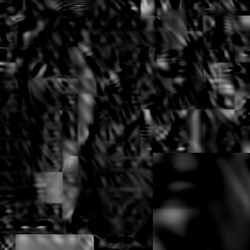
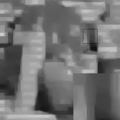
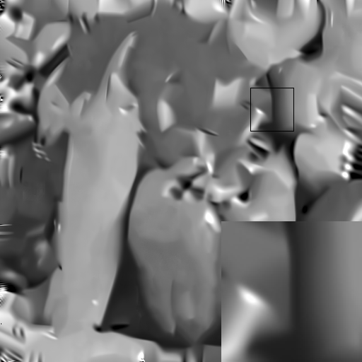
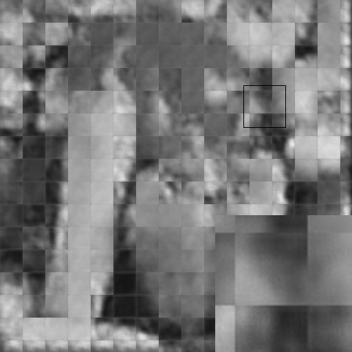
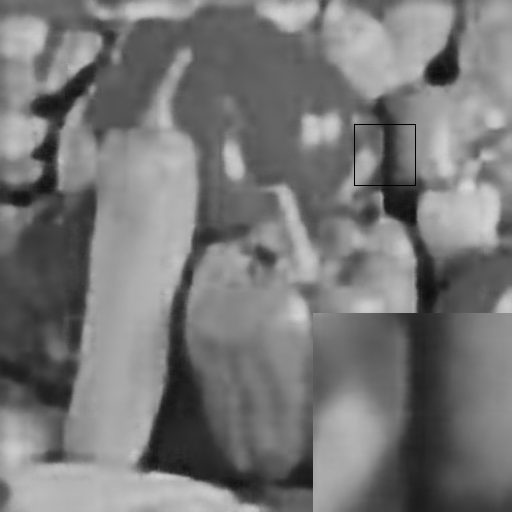
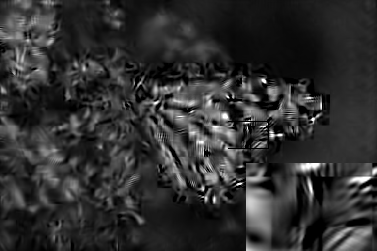
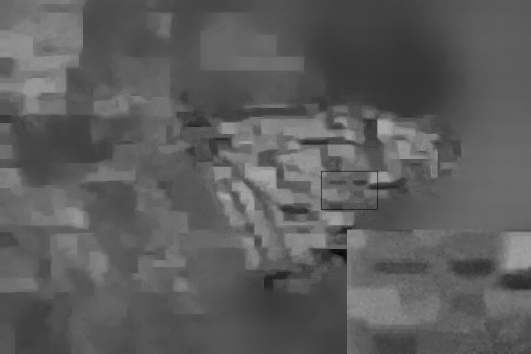
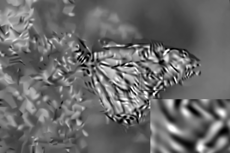
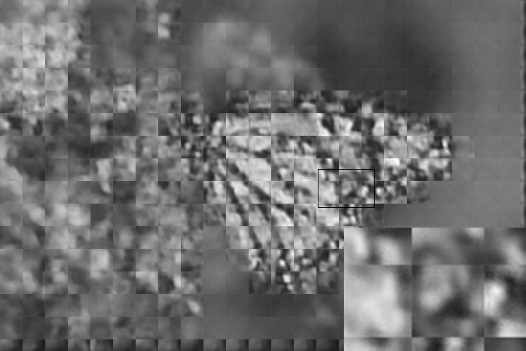
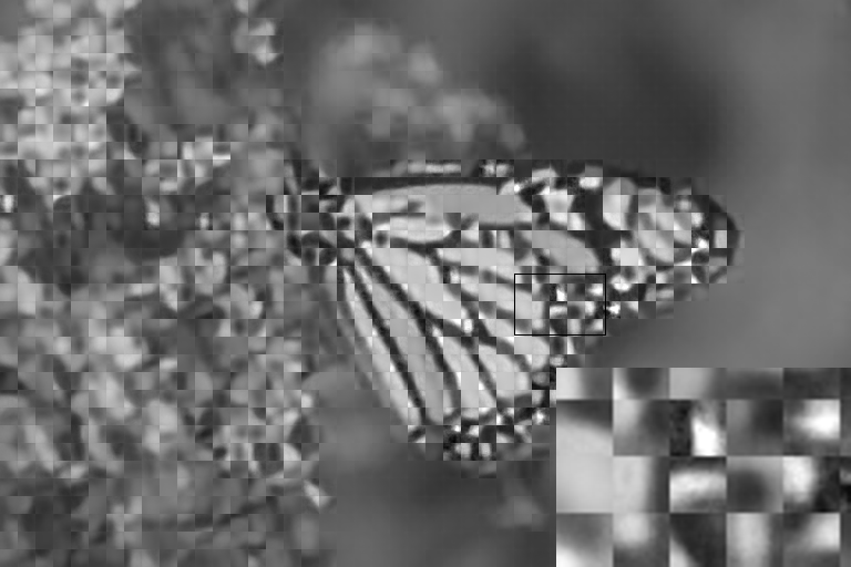
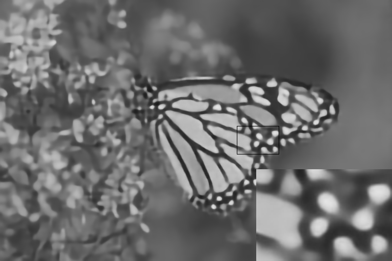
We compare our algorithm with seven representative methods, i.e., total variation (TV) method [5], multi-hypothesis (MH) method [13], collaborative sparsity (Cos) method [14], group sparse representation (GSR) method [6], ReconNet [8], BCSNet [9] and CSNet [3]. In these algorithms, the first four belong to traditional optimization-based methods, while the last three are recent network-based methods. The PSNR and SSIM reconstruction performances at three different sampling ratios: 0.01, 0.02 and 0.1 for the datasets Set5 and Set14 are summarized in Table 1 and Table 2, respectively. The “LapCSNet-2” denotes and “LapCSNet-4” . It can be seen from the tables that about 0.2-0.5dB PSNR improvement is obtained on both test datasets Set5 and Set14 when the sampling ratio is very low. Obviously, the proposed method outperform the existing algorithms in low-ratio by a large margin, which fully demonstrates the effectiveness of our model. Moreover, for the ratio=0.01, our model is about 4 times deeper than CSNet, while the running time is just about 3 times longer than that of the CSNet, which demonstrate the Laplacian pyramid is a high-efficiency design for CS reconstruction. The visual comparisons in the case of ratio=0.01 and ratio=0.02 in Fig. 2 and Fig. 3 show that the proposed LapCSNet is able to reconstruct more details and sharper edges without obvious blocking artifacts.
4 CONCLUSION
In this work, we propose a deep convolutional network (LapCSNet) within a Laplacian pyramid framework for fast and accurate CS reconstruction. Our model consists of two sub-networks namely sampling sub-network and reconstruction sub-network. In the sampling sub-network, the sampling filters are learned jointly with the reconstruction sub-network. In the reconstruction sub-network, we divide our model into two branches to extract the residual features and integrate target images using laplacian pyramid architectures, respectively. In other words, the reconstruction sub-network progressively predicts high-frequency residuals and integrate multi-scale information in a coarse-to-fine manner. The sampling sub-network and reconstruction sub-network are optimized jointly using a robust Charbonnier loss function. Experimental results show that the proposed LapCSNet is capable of reconstructing more details and sharper edges against several state-of-the-arts algorithms.
5 ACKNOWLEDGEMENTS
This work is partially funded by the Major State Basic Research Development Program of China (973 Program 2015CB351804) and the National Natural Science Foundation of China under Grant No. 61572155 and 61672188.
References
- [1] Emmanuel J Candès, Justin Romberg, and Terence Tao, “Robust uncertainty principles: Exact signal reconstruction from highly incomplete frequency information,” IEEE Transactions on Information Theory, vol. 52, no. 2, pp. 489–509, 2006.
- [2] David L Donoho, “Compressed sensing,” IEEE Transactions on Information Theory, vol. 52, no. 4, pp. 1289–1306, 2006.
- [3] Wuzhen Shi, Feng Jiang, Shengping Zhang, and Debin Zhao, “Deep networks for compressed image sensing,” IEEE International Conference on Multimedia and Expo (ICME), pp. 877–882, 2017.
- [4] Scott Shaobing Chen, David L Donoho, and Michael A Saunders, “Atomic decomposition by basis pursuit,” SIAM review, vol. 43, no. 1, pp. 129–159, 2001.
- [5] Chengbo Li, Wotao Yin, Hong Jiang, and Yin Zhang, “An efficient augmented lagrangian method with applications to total variation minimization,” Computational Optimization and Applications, vol. 56, no. 3, pp. 507–530, 2013.
- [6] Jian Zhang, Debin Zhao, and Wen Gao, “Group-based sparse representation for image restoration,” IEEE Transactions on Image Processing, vol. 23, no. 8, pp. 3336–3351, 2014.
- [7] Ali Mousavi, Ankit B Patel, and Richard G Baraniuk, “A deep learning approach to structured signal recovery,” IEEE Allerton Conference on Communication, Control, and Computing (Allerton), pp. 1336–1343, 2015.
- [8] Kuldeep Kulkarni, Suhas Lohit, Pavan Turaga, Ronan Kerviche, and Amit Ashok, “Reconnet: Non-iterative reconstruction of images from compressively sensed random measurements,” IEEE Conference on Computer Vision and Pattern Recongnition (CVPR), pp. 449–458, 2016.
- [9] Amir Adler, David Boublil, Michael Elad, and Michael Zibulevsky, “A deep learning approach to block-based compressed sensing of images,” arXiv preprint arXiv:1606.01519, 2016.
- [10] Andrés Bruhn, Joachim Weickert, and Christoph Schnörr, “Lucas/kanade meets horn/schunck: Combining local and global optic flow methods,” Springer International Journal of Computer Vision, vol. 61, no. 3, pp. 211–231, 2005.
- [11] Kaiming He, Xiangyu Zhang, Shaoqing Ren, and Jian Sun, “Deep residual learning for image recognition,” IEEE Conference on Computer Vision and Pattern Recognition, pp. 770–778, 2016.
- [12] Vincent Dumoulin and Francesco Visin, “A guide to convolution arithmetic for deep learning,” arXiv preprint arXiv:1603.07285, 2016.
- [13] Chen Chen, Eric W Tramel, and James E Fowler, “Compressed-sensing recovery of images and video using multihypothesis predictions,” IEEE Conference Record of the Forty Fifth Asilomar Conference on Signals, Systems and Computers (ASILOMAR), pp. 1193–1198, 2011.
- [14] Jian Zhang, Debin Zhao, Chen Zhao, Ruiqin Xiong, Siwei Ma, and Wen Gao, “Compressed sensing recovery via collaborative sparsity,” IEEE Data Compression Conference (DCC), pp. 287–296, 2012.
- [15] Kaiming He, Xiangyu Zhang, Shaoqing Ren, and Jian Sun, “Delving deep into rectifiers: Surpassing human-level performance on imagenet classification,” IEEE International Conference on Computer Vision, pp. 1026–1034, 2015.
- [16] Pablo Arbelaez, Michael Maire, Charless Fowlkes, and Jitendra Malik, “Contour detection and hierarchical image segmentation,” IEEE Transactions on Pattern Analysis and Machine Intelligence, vol. 33, no. 5, pp. 898–916, 2011.
- [17] Andrea Vedaldi and Karel Lenc, “Matconvnet: Convolutional neural networks for matlab,” ACM International Conference on Multimedia, pp. 689–692, 2015.