Existence of Compact Structures in $f(R,T)$ Gravity

Abstract

The present paper is devoted to investigate the possible emergence of relativistic compact stellar objects through modified $f(R,T)$ gravity. For anisotropic matter distribution, we used Krori and Barura solutions and two notable and viable $f(R,T)$ gravity formulations. By choosing particular observational data, we determine the values of constant in solutions for three relativistic compact star candidates. We have presented some physical behavior of these relativistic compact stellar objects and some aspects like energy density, radial as well as transverse pressure, their evolution, stability, Eos parameters, measure of anisotropy and energy conditions.

Keywords: Gravitation; Stability; Relativistic dissipative fluids
PACS: 04.40.-b, 04.40.Nr, 04.40.Dg

1 Introduction

General relativity (GR) is considered as the most fruitful theory for understanding the evolution of universe and its hidden secrets, yet the evidence of dark matter (DM) and the cosmic accelerating nature of spacetime put some challenges on this [1, 2, 3, 4, 5, 6, 7]. The Einstein’s GR explained the cosmological phenomena in a regime of weak field, while some modifications may be needed to study the strong fields in the scenario of accelerating expansion of the universe. In this direction, Qadir et al. [8] reinforced the requirement of the modified relativistic dynamics and indicated that this modification may help to settle down the problems related to DM and quantum gravity. As a result, many techniques were used like by introducing the cosmological constant as well as the modified theories from time to time.

Modified gravitational theories (MGTs) are actually the generalization of GR in which function of the Ricci scalar ($R$) is substituted in the Einstein-Hilbert action. These modified gravity theories are dubbed with the names, Einstein-$\Lambda$ [9], $f(R)$ [10] ($R$ is the Ricci scalar), $f(R,T)$ [11] ($T$ is the trace of energy momentum tensor), $f(G)$ [12] ($G$ is the Gauss-Bonnet term) and $f(R,T,R_{\xi\pi}T^{\xi\pi})$ gravity [13]. In the recent times, Nojiri et al. [14] presented various mathematical techniques to understand burning issues of cosmos related to bouncing cosmos. They asserted that gravity mediated by $f(R)$ and $f(G)$ theories could be used to realize many hidden secrets of our universe. Once can observe the pity good agreement results between the cosmological models in MGTs and the observational data [15, 16, 17, 18]. The $f(R,T)$ gravity is one of the MGTs, in which the $f(R)$ is replaced with the function of $R$ and $T$ [19]. It is claimed that the evidence behind the dependence of $T$ may come from the presence of imperfect fluid or it may be some kinds of quantum effects (for further reviews on DE and MGTs, see, for instance, [20, 21, 22, 23, 24, 25, 26, 27, 28, 29, 30, 31, 32]).

In $f(R,T)$ gravity, many cosmological applications were discussed in [33, 34, 35, 36, 37, 38]. From literature, some of them are, The non-static line element for collapsing of spherical body having anisotropic fluid were discussed in [39]. The static spherical wormhole solutions were found in [40, 41]. Furthermore, the perturbation techniques were used in study of spherical stars [42]. The effects on gravitational lensing due to $f(R,T)$ gravity were discussed in [43]. The spherical equilibrium theme of polytropic and strange stars were investigated in [44]. Houndjo [45] constructed few observationally notable cosmic models in $f(R,T)$ gravity for studying matter dominated era of the expanding universe. Baffou et al. [46] applied perturbation on the spacetimes of de-Sitter and power law models in order to explore some cosmic viability bounds.

Bamba et al. [47] analyzed the effects of higher degrees of freedom coming from MGT on the dynamical features of our accelerating cosmos. Bamba et al. [53] further checked the viability regimes on the parameters of $f(G)$ gravity models and presented some mathematically consistent cosmic zones. The stability of gravitational evolving stellar bodies have been investigated in few models of $f(R)$ gravity by [49, 51]. Das et al. [52] calculated exact relativistic models of spherical interiors in MGT and discussed the physical implications of their results on compact stars.

Yousaf and his collaborators examined the role of various curvature invariant functions on the existence as well as stability of the planar [54], spherical [55] and cylindrical [56] geometries. Sahoo with his coworkers [57] studied the viability of the spatially regular cosmos along with some other cosmological aspects in $f(R,T)$ gravity. Moraes et al. [58] worked out the stability of some well-known compact stars by computing their corresponding hydrostatic equations in $f(R,T)=R+2\lambda T$ gravity.

The exploration on the existence of self-gravitating compact stars have always been a source of great attention among gravitational physicists. [59, 60, 61, 62, 63, 64, 65, 66]. In this direction, many researchers reconstructed different models for the study of anisotropic relativistic compact stars. Various physical properties, like masses of compact stars, radii, stability etc. and the moment of inertia of neutron stars were studied with the comparison developed with GR and other MGTs [67]. Virbhadra et al. [68, 69] discussed the relation between naked singularity and black holes formation accompanied with a well-consistent mathematical stand point. Egeland [81] performed the modeling of neutron star by examining some mass radius relations and concluded that $\Lambda$ should exist to justify the vacuum density. Sharif and Yousaf [70] also found these relations and checked the existence of compact structures in the platform of MGTs. Bhatti et al. [71] calculated dark dynamical variables and checked the dynamics of compact stars with the help of these variables. Recently, Yousaf et al. [72] investigated the stability of three different compact structures in the presence of dark sources terms mediated by quadratic, cubic and exponential $f(R)$ formulations.

Here, we use the modified $f(R,T)$ gravity, which can be considered as more well established theory than that of cosmological constant. To explore the formation of relativistic anisotropic compact stellar objects in $f(R,T)$ gravity, we use two such a viable $f(R,T)$ models for three candidates of strange stars, i,e., Her X-1, SAXJ1808.4-3658 and 4U1820-30. We shall label these stars with CS1, CS2 and CS3, respectively. We find the solutions of relativistic anisotropic stellar bodies in $f(R,T)$ gravity, that enforce some constraints on the cosmic model parameters. In very next section, we formulate $f(R,T)$ equation of motions, after having the background of $f(R,T)$ gravity, we take anisotropic matter contents for static spherical star geometry. In section 3, we demonstrate some of the physical viable models in $f(R,T)$ gravity. In section 4, we explore the solutions and discussed the physical properties of relativistic compact stars through graphical illustrations. At the end, we finalize our results.

2 $f(R,T)$ gravity

The action for $f(R,T)$ gravity can be written as

$$I=\int{d{x^{4}}\sqrt{-g}\left[{f(R,T)+{L_{matter}}}\right]},$$ (2.1)

where $g$ and $L_{matter}$ indicate determinant of metric tensor and the matter Lagrangian, respectively. By varying the above equation with metric tensor, we get

$${R_{\xi\pi}}{f_{R}}-\frac{1}{2}{g_{\xi\pi}}f+\left({{g_{\xi\pi}}{\nabla^{\xi}}{\nabla_{\mu}}-{\nabla_{\mu}}{\nabla_{\pi}}}\right){f_{R}}$$

$$={T_{\xi\pi}}-{f_{T}}{\Theta_{\xi\pi}}-{f_{T}}{T_{\xi\pi}},$$ (2.2)

where the notations ${f_{R}},~{}{\nabla_{\gamma}}$ and ${f_{T}}$ are operators for covariant and partial derivatives of their arguments, respectively, while ${\Theta_{\mu\nu}}$ can be expressed through the stress-energy tensor ($T_{\gamma\delta}$) as

$${\Theta_{\xi\pi}}=\frac{{{g^{\alpha\beta}}\delta{T_{\alpha\beta}}}}{{\delta{g^{\xi\pi}}}}=-2{T_{\xi\pi}}+{g_{\xi\pi}}{L_{m}}-2{g^{\alpha\beta}}\frac{{{\partial^{2}}{L_{m}}}}{{\partial{g^{\xi\pi}}\partial{g^{\alpha\beta}}}}.$$ (2.3)

The aim of this work is to check the different properties of some of the compact stars with locally anisotropic pressure. Now, we consider that the spherical distribution of geometric system is coupled with the following relativistic fluid

$${T_{\mu\nu}}=(\rho+{P_{t}}){V_{\mu}}{V_{\nu}}-{P_{t}}{g_{\mu\nu}}+\Pi{X_{\mu}}{X_{\nu}},$$ (2.4)

in which $\Pi\equiv P_{r}-P_{\bot}$ and $\rho$ is the matter energy density and ${V_{\gamma}}$ and $X_{\gamma}$ are the 4-vectors corresponding to fluid and radial directions, respectively. Under the non-tilted coordinate system, the four vectors satisfy ${V^{\alpha}}{V_{\alpha}}=1$ and ${X^{\beta}}{X_{\beta}}=-1$ relations. Equation (2.3) can be written, after choosing $L_{m}=\rho$, as

$${\Theta_{\alpha\beta}}=-2{T_{\alpha\beta}}+\rho{g_{\alpha\beta}}$$

Then, the field equations (2.2) boil down to

$${R_{\xi\pi}}-\frac{1}{2}R{g_{\xi\pi}}=T_{\xi\pi}^{\textrm{eff}},$$ (2.5)

where $T_{\xi\pi}^{\textrm{eff}}$ is dubbed with the effective stress energy tensor for $f(R,T)$ gravity whose mathematical formulations is given by

$$\begin{gathered}T_{\xi\pi}^{\textrm{eff}}=\frac{1}{{{f_{R}}}}\left[{(1+{f_{T}})}\right.{T_{\xi\pi}}-\rho{g_{\xi\pi}}{f_{R}}+\frac{1}{2}(f-R{f_{R}}){g_{\xi\pi}}+({\nabla_{\xi}}{\nabla_{\pi}}-{g_{\xi\pi}}{\nabla^{\alpha}}{\nabla_{\alpha}})\left.{f_{R}}\right].\end{gathered}$$ (2.6)

Now, we wish to consider the diagonally symmetric static form of spherically symmetric spacetime as

$$d{s^{2}}={e^{a}}d{t^{2}}-{e^{b}}d{r^{2}}-{r^{2}}\left({d{\theta^{2}}+{{\sin}^{2}}\theta d{\phi^{2}}}\right),$$ (2.7)

where metric coefficients $a$ and $b$ are the $r$ dependent functions. Our aim is to analyze the role of anisotropicity in the modeling of some stellar toy models. So, we assume that Eq.(2.7) is composed of the locally anisotropic fluid content given in Eq.(2.4). The $f(R,T)$ equations of motion (2.2) for the geometry (2.7) and fluid (2.4) yield

$$\rho ={e^{-b}}\left[{\left\{\frac{1}{4}a^{\prime}{{(r)}^{2}}+{\frac{{a^{\prime\prime}}}{2}-\frac{b^{\prime}}{4}a^{\prime}+\frac{{a^{\prime}}}{r}}\right\}{f_{R}}\left({R,T}\right)}+\left({\frac{{b^{\prime}(r)}}{2}-\frac{2}{r}}\right)\right.\left.{{f_{R}}^{\prime}-\frac{{f_{R}}}{2}{e^{b}}-{f_{R}}{{{}^{\prime}}^{\prime}}}\right],$$ (2.8)

$$P_{r} =\frac{{{e^{-b}}}}{{\left({1+{f_{T}}\left({R,T}\right)}\right)}}\left[{\left\{{-\frac{{a^{\prime\prime}}}{2}-\frac{b^{\prime}}{4}a^{\prime}+\frac{{b^{\prime}}}{r}}-\frac{1}{4}a^{\prime 2}\right\}{f_{R}}}\right.\left.{+\left({\frac{{a^{\prime}}}{2}+\frac{2}{r}}\right){f_{R}}^{\prime}+\frac{{e^{b}}}{2}{f_{R}}}\right]-\frac{{\rho{f_{T}}}}{{\left({1+{f_{T}}}\right)}},$$ (2.9)

$$P_{t} =\frac{{{e^{-b}}}}{{\left({1+{f_{T}}}\right)}}\left[{\left\{{e^{b}}+{\frac{r}{2}\left({b^{\prime}-a^{\prime}}\right)-1}\right\}\frac{{{f_{R}}}}{{{r^{2}}}}}+\left\{-\frac{1}{2}({b^{\prime}-a^{\prime}})\right.\right.\left.\left.+\frac{1}{r}\right\}{{f_{R}}^{\prime}+{f_{R}}^{\prime\prime}+\frac{{f_{R}}}{2}{e^{b}}}\right]$$

$$-\frac{{\rho{f_{T}}}}{{\left({1+{f_{T}}}\right)}},$$ (2.10)

where the over prime indicates $\partial/\partial r$ operator.

In order to analyse the impact of $f(R,T)$ gravity on the construction of stellar models, we assume the separable form of $R$ and $T$ in $f(R,T)$ model as follows

$$f(R,T)=f_{i}(R)+g(T).$$ (2.11)

This choice of separable $R$ and $T$ can be regarded as a possible linear corrections in the well-known $f(R)$ theory. By choosing $f_{i}(R)$ from [16] along with the linear combination of $g(T)$, the viable $f(R,T)$ model can be designed. Therefore, we suppose $g(T)=\epsilon T$ in which $\epsilon$ is a very small positive number. In this context, Eqs.(2.8)-(2.10) provide

$$\rho =\frac{1}{{2(1+2\epsilon)}}\left[{\frac{{(2+5\epsilon)}}{{(1+\epsilon)}}{\varphi_{1}}+\epsilon{\varphi_{2}}+2\epsilon{\varphi_{3}}}\right],$$ (2.12)

$$P_{r} =\frac{{-1}}{{2(2\epsilon+1)}}\left[{\frac{\epsilon}{{\left({\epsilon+1}\right)}}{\varphi_{1}}-(2+3\epsilon){\varphi_{2}}+2\epsilon{\varphi_{3}}}\right],$$ (2.13)

$$P_{t} =\frac{{-1}}{{2(1+2\epsilon)}}\left[{\frac{\epsilon}{{(1+\epsilon)}}{\varphi_{1}}+\epsilon{\varphi_{2}}-2(1+\epsilon){\varphi_{3}}}\right],$$ (2.14)

where

$${\varphi_{1}} ={e^{-b}}\left[{\left({\frac{a^{\prime 2}}{4}+\frac{{a^{\prime\prime}}}{2}-\frac{b^{\prime}}{4}a^{\prime}+\frac{{a^{\prime}}}{r}}\right){f_{R}}}+\left({\frac{{b^{\prime}}}{2}-\frac{2}{r}}\right)\right.\left.{\times{f_{R}}^{\prime}-\frac{{f_{R}}}{2}{e^{b}}-{f_{R}}^{\prime\prime}}\right],\hfill$$

$${\varphi_{2}} =\frac{{{e^{-b}}}}{{\left({1+\epsilon}\right)}}\left[{\left({\frac{{b^{\prime}}}{r}-\frac{{a^{\prime\prime}}}{2}-\frac{b^{\prime}}{4}a^{\prime}-\frac{1}{4}a^{\prime 2}}\right){f_{R}}}+\left({\frac{2}{r}+\frac{{a^{\prime}}}{2}}\right)\right.\left.{\times{f_{R}}^{\prime}+\frac{1}{2}{e^{b}}{f_{R}}}\right],\hfill$$

$${\varphi_{3}} =\frac{{{e^{-b}}}}{{\left({1+\epsilon}\right)}}\left[{\left({{e^{b}}-\frac{1}{2}r\left({a^{\prime}-b^{\prime}}\right)-1}\right)\frac{{{f_{R}}}}{{{r^{2}}}}}+\left\{{\frac{1}{r}-\frac{1}{2}\left({b^{\prime}-a^{\prime}}\right)}\right\}{{f_{R}}^{\prime}+\frac{{f_{R}}}{2}{e^{b}}+{f_{R}}^{\prime\prime}}\right].$$

We write $a$ and $b$ as a combinations of radial coordinates suggested by Krori and Barua [82]. They proposed the specific forms of these functions as $a(r)=Br^{2}+C$ and $b(r)=Ar^{2}$, where $A,~{}B$ and $C$ are the three constant numbers. One can find the values of this triplet $(A,~{}B,~{}C)$ by considering some appropriate boundary conditions. Then, Eqs.(2.12)-(2.14) yield

$$\rho =\frac{{{{\rm{e}}^{-A{r^{2}}}}}}{{2{r^{2}}\left({1+\epsilon}\right)\left({1+2\epsilon}\right)}}[-{{\rm{e}}^{A{r^{2}}}}{r^{2}}\left({1+\epsilon}\right)f_{i}+(2(-1-2\epsilon+3B{r^{2}}\epsilon+{B^{2}}{r^{4}}\epsilon+{{\rm{e}}^{A{r^{2}}}}$$

$$\times\left({1+2\epsilon}\right)+A{r^{2}}\left({2+4\epsilon-B{r^{2}}\epsilon}\right))+{{\rm{e}}^{A{r^{2}}}}{r^{2}}(1+\epsilon)R)f_{i}^{\prime}+r((-4-6\epsilon+3B{r^{2}}\epsilon$$

$$+A{r^{2}}(2+3\epsilon)){R^{\prime}}f_{i}^{\prime\prime}-r\left({2+3\epsilon}\right){R^{\prime\prime}}f_{i}^{\prime\prime}-r\left({2+3\epsilon}\right){R^{\prime}}^{2}f_{i}^{\prime\prime\prime})],$$ (2.15)

$${P_{r}} =\frac{{{{\rm{e}}^{-A{r^{2}}}}}}{{2{r^{2}}\left({1+\epsilon}\right)\left({1+2\epsilon}\right)}}[{{\rm{e}}^{A{r^{2}}}}{r^{2}}\left({1+\epsilon}\right)f_{i}-(2(-1-2\epsilon+{B^{2}}{r^{4}}\epsilon+{{\rm{e}}^{A{r^{2}}}}(1+2\epsilon)$$

$$-B{r^{2}}\left({2+\epsilon+A{r^{2}}\epsilon}\right))+{{\rm{e}}^{A{r^{2}}}}{r^{2}}\left({1+\epsilon}\right)R)f_{i}^{\prime}+r[\{4+6\epsilon+A{r^{2}}\epsilon+B{r^{2}}(2+\epsilon)\}$$

$$\times R^{\prime}f_{i}^{\prime\prime}-r\epsilon R^{\prime\prime}f_{i}^{\prime\prime}-r\epsilon R^{\prime 2}f_{i}^{\prime\prime\prime}]],$$ (2.16)

$${P_{t}} =\frac{{{{\rm{e}}^{-A{r^{2}}}}}}{{2{r^{2}}\left({1+\epsilon}\right)\left({1+2\epsilon}\right)}}[{{\rm{e}}^{A{r^{2}}}}r\left({1+\epsilon}\right)fi-r[2\{-B(2+\epsilon+B{r^{2}}(1+\epsilon))+A(1+2\epsilon$$

$$+B{r^{2}}(1+\epsilon))\}+{{\rm{e}}^{A{r^{2}}}}\left({1+\epsilon}\right)R]f_{i}^{\prime}+2{R^{\prime}}f{i^{\prime\prime}}-2A{r^{2}}{R^{\prime}}f{i^{\prime\prime}}+2B{r^{2}}{R^{\prime}}f{i^{\prime\prime}}+2\epsilon R^{\prime}f_{i}^{\prime\prime}$$

$$-3A{r^{2}}\epsilon R^{\prime}f_{i}^{\prime\prime}+B{r^{2}}\epsilon R^{\prime}f_{i}^{\prime\prime}+2f_{i}^{\prime\prime}rR^{\prime\prime}+3r\epsilon R^{\prime\prime}f_{i}^{\prime\prime}+2r{R^{\prime}}^{2}f_{i}^{\prime\prime\prime}+3r\epsilon R^{\prime 2}f_{i}^{\prime\prime\prime}].$$ (2.17)

3 Boundary Conditions

We consider a timelike hypersurface denoted by $\Omega$ that has differentiated interior manifold given in Eq.(2.7) and outer geometry. The exterior region is through the vacuum Schwarzschild spacetime as

$$d{s^{2}}=\left({1-\frac{{2M}}{r}}\right)d{t^{2}}-{\left({1-\frac{{2M}}{r}}\right)^{-1}}d{r^{2}}-{r^{2}}\left({d{\theta^{2}}+{\mathop{\rm\sin}\nolimits}{\theta^{2}}d{\varphi^{2}}}\right),$$ (3.1)

where $M$ is the gravitating matter content. At the boundary surface $\Omega$, the continuity of the metric variables $g_{tt},~{}g_{rr}$ and the $\partial g_{tt}/\partial r$ provide the following constraints

$$A =\frac{{-1}}{{{R^{2}}}}\ln\left({1-\frac{{2M}}{R}}\right),\quad B=\frac{M}{{{R^{3}}}}{\left({1-\frac{{2M}}{R}}\right)^{-1}},$$ (3.2)

$$C =\ln\left({1-\frac{{2M}}{R}}\right)-\frac{M}{R}{\left({1-\frac{{2M}}{R}}\right)^{-1}}.$$ (3.3)

For the smooth and continuous matching of the manifolds, the above constraints at $\Omega$ should be fulfilled. We now pick some observational values of $A,~{}B$ and $C$ from the literature to check the construction as well as the stability of the compact stellar bodies. We consider, three stellar toy models Her X-1, SAXJ1808.4-3658 and 4U1820-30 labeled with CS1, CS2 and CS3 here. The masses of these star candidates are $0.88$, $1.435$ and $2.25$ solar masses, respectively. All of these stellar structures satisfy Buchdahl Bondi bound as their $2M/R$ ratios are less than $8/9$. We further suppose that the junction conditions at the stellar core are [84]

$$\rho(r)={\rho_{c}}$$ (3.4)

$$\frac{{da}}{{dr}}(0)=0,$$ (3.5)

$$b(0)=0,$$ (3.6)

where $\rho_{c}$ is the critical mass density.

Compact Stars (CS)	$R(km$	$M$	$\mu=\frac{M}{R}$	$B(km^{-2})$	$A(km^{-2})$
CS1	$7.7$	$0.88M_{\odot}$	$0.168$	$0.004267364618$	$0.006906276428$
CS2	$7.07$	$1.435M_{\odot}$	$0.299$	$0.01488011569$	$0.01823156974$
CS3	$10$	$2.25M_{\odot}$	$0.332$	$0.009880952381$	$0.01090644119$

Table 1: The observational values of the radii $R$, masses $M$, compactness $\mu$, and the constants $B$ and $A$ for CS1, CS2 and CS3.

4 Various $f(R,T)$ Models

The aim of this section is to study some of the notable $f(R,T)$ models. We want to analyze the influences of these $f(R,T)$ models in the construction and stability of the compact stellar candidates in the background of some observations. We shall discuss some realistic features of spherical systems like, compactness, stability, evolution of energy density with radial coordinate, the measurement of anisotropic pressure evolution and the different energy conditions. The results obtained such investigations may provide some hidden realities corresponding to the both theoretical and astrophysical regimes. Equation (2.11) provides

$$f(R,T)=fi(R)+\epsilon T,$$ (4.1)

where $i=1,~{}2$. There has been very interesting results which reveal that the inclusion of extra dark energy/DM components mediated from alternative theories could bring some exciting results. For instance, collapse time, existence of more compact structure, stability, phenomenon of core formation and above all can be well influenced by these dark source terms unlike GR. The reexamination of GR problems in alternatives theories may be helpful to shed some light on the models viability and their usefulness on physical grounds. The cross-examinations may present both quantitative and qualitative different consequences than that of GR.

It is of particular interest for many researchers to explore the predictions as well as the outcomes of modified gravitational theories like $f(R,T)$ theory concerning the existence of stellar structure and their stability. The $f(R,T)$ gravity can be treated as a mathematical tool to examine various unknown features of gravitational dynamics at large scales. Schaefer and Koyama [88] generalized their study of gravitational collapse of spherical structures in the realm of modified gravity and Birkhoff-theorem and found enhanced cluster merging rates as well as overdensed populations of relativistic structures (due to modified gravity). Capozziello et al. [89] computed modified Lané-Emden expression with metric $f(R)$ corrections and Newtonian approximation. They get some exceptional results of density and pressure distribution in the analysis of the hydrostatic scenario of few celestial bodies. Cembranos et al. [90] studied stellar structure formation in the background of modified gravity and found comparatively higher contraction in the collapsing rate of spherical systems at its initial stages unlike GR.

Astashenok et al.[91] examined the impact of few modified gravity formulations on the existence of compact structure and inferred that there exists some models whose corrections could lead arena of having relatively more compact stars than in GR. Yousaf and Bhatti [77] studied the influences of modified dark source terms on mass-radius relationships for compact stars and concluded that some extended gravities mediated by Lagrangians $\alpha R^{2}$ and $\frac{\alpha R^{2}-\beta R}{1+\gamma R}$ are likely to host supermassive relativistic systems with comparatively smaller radii than in GR. Resco et al. [92] numerically calculated apparent masses of neutron star models in modified gravity and inferred that generically some modified extra degrees of freedom likely to keep significantly massive neutron star with smaller radii than in GR. Such type of investigations could provide theoretical well-consistent way to handle and study classes of massive and super massive structures at large scales. Bamba et al. [93] claimed that modified gravitational dynamics could provide an additional platform in few regions of spacetime that could lead to stable configurations of relativistic system. In this paper, we found relatively stellar bodies with much higher densities than that found in GR [80] as seen from Fig.(2).

In the following we discuss two different $f(R,T)$ models.

4.1 Model 1

Firstly, we take the tanh modification of the Ricci scalar function that was proposed by [85]. In this respect, the $f(R,T)$ gravity model (4.1) give

$$f(R,T)=R-\alpha\hat{R}\tanh\left(\frac{R}{\hat{R}}\right)+\epsilon T,$$ (4.2)

where $\alpha\in\mathbb{R}^{+}$ and $\hat{R}\in\mathbb{R}^{+}$ in which $\mathbb{R}^{+}$ denotes the set of positive real numbers. On setting $\alpha=0$, the dynamics of Einstein s gravity can be discussed.

4.2 Model 2

Next, we consider another viable formulations of $f(R)$ gravity that was first suggested by [86]. Under this context, Eq.(4.1) becomes

$$f(R,T)=R+\gamma\hat{R}\left((1+\frac{R^{2}}{\hat{R^{2}}})^{-q}-1\right)+\epsilon T,$$ (4.3)

where $\hat{R},~{}\gamma$ and $q$ are the free non zero and non negative parameters.

In the coming section, we will use these two viable model for further investigation of compact stars.

5 Some Physical Properties

This section is devoted to analyze various aspects of some compact stellar toy models. We assume three different star distributions, i.e., CS1, CS2, CS3 as well as two observationally consistent $f(R,T)$ models. Upon substituting this data in Eqs.(2.8)-(2.10), we get values of matter variables in the form of four parameters, $\alpha,~{}\hat{R},~{}q$ and $\epsilon$. Then, we study some physical features to obtain the realistic configurations of compact stellar structures (shown in Table 1). The comparison between our theoretical outcomes and the observational data may provide the strong evidences for $f(R,T)$ models. We shall show our results with the help of plots.

5.1 Density and Pressure Evolutions

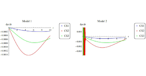
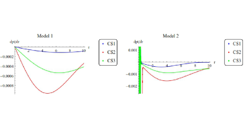
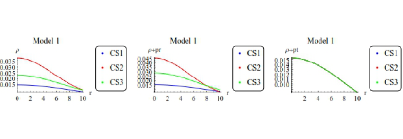
This section is devoted to analyze the matter parameters of all the three stellar bodies whose variations are depending on the radial coordinate. We check the radial variations in the anisotropic pressure, energy density and their corresponding radial derivatives. Now with the help of Eqs.(2.8)-(2.10), we plot diagrams (2) for all the three stellar models in the background of two above mentioned $f(R,T)$ models¿ We infer that the behavior of energy densities keep on increasing till the constraint $r\rightarrow 0$. This indicates the distribution of $\rho$ to be increasing with respect to the decreasing choices of $r$. One can say from these that our stellar toy models are of having highly compact cores in the degrees of freedom coming from Eqs.(4.2) and (4.3). The Figures (2) and (3) describe the plots of the variations in the components of the star pressure.

Figure 1: Graph for the density ($km^{-2}$) evolution with both $f(R,T)$ models.

Figure 2: Graph for the radial pressure ($km^{-2}$) evolution with both $f(R)$ models.

Figure 3: Graph for the transverse pressure ($km^{-2}$) evolution with both $f(R,T)$ models.

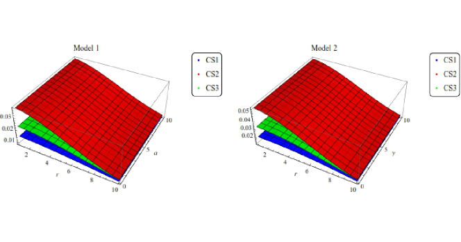
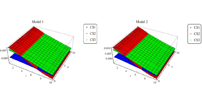
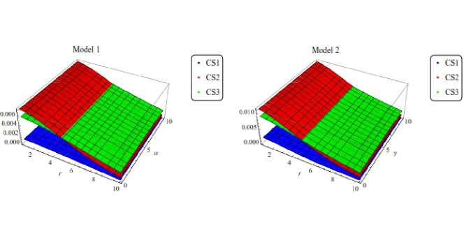
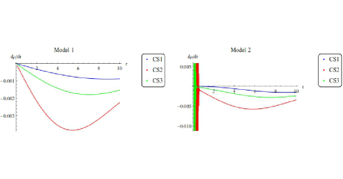
Furthermore, Figures (6), (6) and (6) are describing the variations in the $r$ derivative of $\rho$ and $p_{i}$. One can observe from these that $\frac{d\rho}{{dr}}<0,~{}\frac{dp_{r}}{{dr}}<0$ and $\frac{dp_{t}}{{dr}}<0$ for the given two viable models and the three toy models. Under the constraint $r=0$, one can notice that the $r$ variations of all the matter variables vanishes, such that

$$\frac{d\rho}{{dr}}=0,$$

$$\frac{dp_{r}}{{dr}}=0.$$

Furthermore, the twice variations of these structural quantities have been found to be negative. These consequences are providing a seed for the high compact profiles of such star structures around their subsequent cores, thus indicating that the configurations of compact and dense stars do exists in the arena of $f(R,T)$ gravity.

Figure 4: Graph describing $d\rho/dr$ with respect to $r$ for both $f(R)$ models.

Figure 5: Graph describing $dp_{r}/dr$ with increasing $r$ for both $f(R)$ models.

Figure 6: Graph describing $dp_{t}/dr$ with increasing $r$ for both $f(R)$ models.

5.2 Energy Conditions

For a realistic matter content distribution, one need to check some particular conditions, such a mathematical conditions are called energy conditions (ECs). These mathematical conditions are the coordinate-invariant. In the regime of modified $f(R,T)$ gravity like the effective forms of density and the anisotropic pressure, the null energy Condition (NEC) and the weak energy conditions (WEC) are devised, respectively, as

$$\bullet\textrm{NEC}\Leftrightarrow{\rho^{\textrm{eff}}}+{P_{i}^{\textrm{eff}}}\geq 0,$$

$$\bullet\textrm{WEC}\Leftrightarrow{\rho^{\textrm{eff}}}\geq 0\text{ and }{\rho^{\textrm{eff}}}+{P_{i}^{\textrm{eff}}}\geq 0,$$

while the rest of ECs, i.e., strong energy condition (SEC) and dominant energy condition (DEC) give

$$\bullet\textrm{SEC}\Leftrightarrow{\rho^{\textrm{eff}}+2{P_{t}^{\textrm{eff}}}+3{P_{r}^{\textrm{eff}}}}\geq 0\text{ and }{\rho^{\textrm{eff}}}+{P_{i}^{\textrm{eff}}}\geq 0,$$

$$\bullet\textrm{DEC}\Leftrightarrow{\rho^{\textrm{eff}}}\geq 0\text{ and }{\rho^{\textrm{eff}}}\pm{P_{i}^{\textrm{eff}}}\geq 0.$$

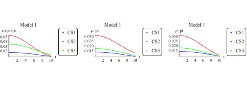
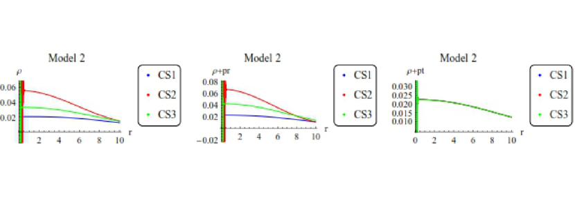
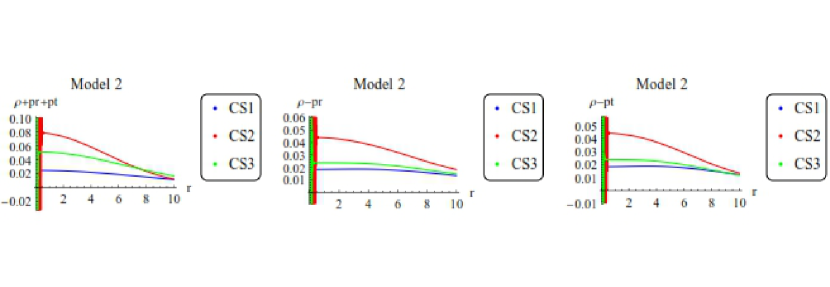
It has been easily be figure out from the plots shown in Figures (7) and (8) that our under considerations of both models with CS1, CS2 and CS3 obey all ECs. This suggests that anisotropic fluid content (2.4) describes the realistic source of gravitational effects.

Figure 7: ECs Viability for three stellar bodies with $f(R,T)=R-\alpha\hat{R}\tanh\left(\frac{R}{\hat{R}}\right)+\epsilon T$

Figure 8: ECs Viability for three stellar bodies with $f(R,T)=R+\gamma\hat{R}\left((1+\frac{R^{2}}{\hat{R^{2}}})^{-q}-1\right)+\epsilon T$

5.3 TOV Equation

A mathematical expression that provide some restrictions on the geometrical distributions of the relativistic spherical system, which is normally hydrostatic equilibrium and is often called as TOV equation. For the spherical line element, this equation is written as

$$\frac{{d{P_{r}}}}{{dr}}+\frac{{a^{\prime}(\rho+{P_{r}})}}{2}+\frac{{2({P_{r}}-{P_{t}})}}{r}=0,$$ (5.1)

The above equation contains three well-known interactions, i.e., the gravitational, $(F_{g})$, hydrostatic, $(F_{h})$ and anisotropic, $(F_{a})$ forces. Therefore, one may write above equation as

$$F_{g}+F_{h}+F_{a}=0.$$ (5.2)

The values of these forces by using of Eqs.(2.8)-(2.10) giives

$$F_{g} \equiv-Br(\rho+P_{r})=\frac{-1}{1+\epsilon}\left[2B\exp(Ar^{2})r\{2(B+A)f_{i}^{\prime}+(B+A)R^{\prime}rf_{i}^{\prime\prime}-R^{\prime\prime}f_{i}^{\prime\prime}-R^{\prime 2}fi^{\prime\prime\prime}\}\right],$$

$$F_{h} \equiv-\frac{{d{p_{r}}}}{{dr}}=\frac{\exp(-Ar^{2})}{2r^{3}(1+\epsilon)(1+2\epsilon)}[4\{1+2\epsilon+B^{2}r^{4}\epsilon+A^{2}Br^{6}\epsilon-\exp(Ar^{2})(1+2\epsilon)+Ar^{2}$$

$$\times(1+2Br^{2}+2\epsilon-B^{2}r^{4}\epsilon)\}fi^{\prime}+r\{-r(4+3(2+Ar^{2})\epsilon+Br^{2}(2+\epsilon))f_{i}^{\prime\prime\prime}R^{\prime 2}+R^{\prime}\{(2$$

$$+8Ar^{2}-6Br^{2}+4ABr^{4}+2\epsilon+11Ar^{2}\epsilon-3Br^{2}\epsilon+2A^{2}r^{4}\epsilon+2B^{2}r^{4}\epsilon+\exp(Ar^{2})(2$$

$$+4\epsilon)+\exp(Ar^{2})r^{2}(1+\epsilon)R)f_{i}^{\prime\prime}+3r^{2}\epsilon R^{\prime\prime}f_{i}^{\prime\prime\prime}\}-f_{i}^{\prime\prime}r((4+6\epsilon+3Ar^{2}\epsilon+Br^{2}(2+\epsilon))R^{\prime\prime}$$

$$-r\epsilon R^{\prime\prime\prime})+r^{2}\epsilon R^{\prime 3}fi^{\prime\prime\prime\prime}\}],$$

$$F_{a} \equiv\frac{{2({P_{r}}-{P_{t}})}}{r}=\frac{2\exp(-Ar^{2})}{r^{3}(1+\epsilon)}[\{\exp(Ar^{2})-(1+Ar^{2}-Br^{2})(1+Br^{2})\}f_{i}^{\prime}+r\{-(1+Ar^{2})$$

$$\times f_{i}^{\prime\prime}R^{\prime}+f_{i}^{\prime\prime}rR^{\prime\prime}+R^{\prime 2}rf_{i}^{\prime\prime\prime}\}].$$

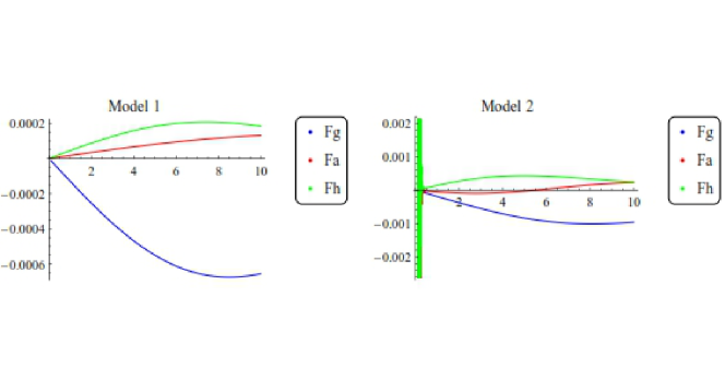
Using above relations together with observational values of $A,~{}B$ and $C$ from Table 1, we have drawn some diagrams mentioned in Figure (9).

Figure 9: Graph describing $F_{g},~{}F_{h}$ and $F_{a}$ with $r$ (km).

In Figure (9), the left plot is for $f(R,T)$ model (4.2) and right plot is for model (4.3). The role of these three types of interactions with respect to $r$ (km) has been seen in this diagram in the modeling of compact bodies CS1, CS2 and CS3.

5.4 Stability Analysis

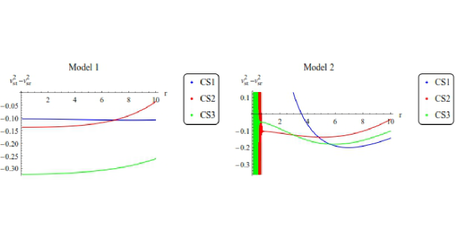
This section illustrates the stability of the compact relativistic structures. It would be interesting to mention that, for any arbitrary relativistic observer, only those stellar bodies are worthy to study which remain in stable position after the application of fluctuations. Thus, the stability problem is among the burning issues for the relativistic astrophysicists. With this intentions, we analyze the stable regimes of our under considerations stellar models by applying the technique developed by [87]. This scheme could be useful to study the phenomenon of cracking. According to this scheme, the stellar system must have the ranges of $v^{2}_{sr}$ and $v^{2}_{st}$ between $0$ and $1$, e.g., in the closed interval $[0,1]$, here $v_{sr}$ and $v_{st}$ represent the radial and transverse sound speeds, respectively. These variables are defined as follows

$$\frac{{d{P_{r}}}}{{d\rho}}=v_{sr}^{2},\quad\frac{{d{P_{t}}}}{{d\rho}}=v_{st}^{2}.$$

Now, using Eqs.(2.8)-(2.10), their values are calculated as

$$v_{sr}=\sqrt{\frac{\chi}{\Psi}},\quad v_{st}=\sqrt{\frac{\phi}{\Psi}},$$

where

$$\chi =r\{4r^{3}(B^{2}(1+\epsilon)+A^{2}(1+2\epsilon+Br^{2}(1+\epsilon))-AB(3+2\epsilon+Br^{2}(1+\epsilon)))f^{\prime}+r\{2(1$$

$$+\epsilon)+Br^{2}(2+\epsilon)-3Ar^{2}(2+3\epsilon)\}R^{\prime 2}fi^{\prime\prime\prime}+R^{\prime}\{(6Br^{2}-2+2B^{2}r^{4}-2\epsilon+3Br^{2}\epsilon+2B^{2}$$

$$\times r^{4}\epsilon+2A^{2}r^{4}(2+3\epsilon)-Ar^{2}(8+11\epsilon+2Br^{2}(3+2\epsilon))-\exp(Ar^{2})r^{2}(1+\epsilon)R\}fi^{\prime\prime}+3r^{2}$$

$$\times(2+3\epsilon)R^{\prime\prime}fi^{\prime\prime\prime}\}+rfi^{\prime\prime}\{(2(1+\epsilon)+Br^{2}(2+\epsilon)-3Ar^{2}(2+3\epsilon))R^{\prime\prime}+r(2+3\epsilon)R^{\prime\prime\prime}\}$$

$$+r^{2}(2+3\epsilon)R^{\prime 3}fi^{\prime\prime\prime\prime}\},$$ (5.3)

$$\Psi =-4[\exp(Ar^{2})(1+\epsilon)-1-2\epsilon-B^{2}r^{4}\epsilon+A^{2}r^{4}\{2+(4-Br^{2})\epsilon\}+Ar^{2}\{-1(4Br^{2}-2$$

$$+B^{2}r^{4})\epsilon\}]fi^{\prime}+r\{r(3(Br^{2}-2)\epsilon-4+3Ar^{2}(2+3\epsilon))R^{\prime 2}fi^{\prime\prime\prime}+R^{\prime}((2+14Ar^{2}-4A^{2}r^{4}+2\epsilon$$

$$+23Ar^{2}(1+\epsilon)fi^{\prime\prime}=3r^{2}(2+3\epsilon)R^{\prime\prime}fi^{\prime\prime\prime})+rfi^{\prime\prime}((3Br^{2}\epsilon-4-6\epsilon+3Ar^{2}(2+3\epsilon))R^{\prime\prime}-r(2$$

$$+3\epsilon)R^{\prime\prime\prime})-r^{2}(2+3\epsilon)R^{\prime 2}fi^{\prime\prime\prime\prime})\},$$ (5.4)

$$\phi =4[4\{1+2\epsilon+B^{2}r^{4}\epsilon+A^{2}Br^{6}\epsilon-\exp(Ar^{2})(1+2\epsilon)+Ar^{2}(1+2Br^{2}+2\epsilon-B^{2}r^{4}\epsilon)\}fi^{\prime}$$

$$+r\{-r(4+3(2+Ar^{2})\epsilon)+Br^{2}(2+\epsilon)\}R^{\prime 2}fi^{\prime\prime\prime}+R^{\prime}\{(2+8Ar^{2}-6Br^{2}+4ABr^{4}+2\epsilon$$

$$+11Ar^{2}\epsilon-3Br^{2}\epsilon+2A^{2}r^{4}\epsilon+2B^{2}r^{4}\epsilon+\exp(Ar^{2})(2+4\epsilon)+\exp(Ar^{2})r^{2}(1+\epsilon)R)fi^{\prime\prime}$$

$$+3r^{2}\epsilon R^{\prime\prime}fi^{\prime\prime\prime}\}-rfi^{\prime\prime}\{(4+6\epsilon+3Ar^{2}\epsilon+Br^{2}(2+\epsilon))R^{\prime\prime}-r\epsilon R^{\prime\prime\prime}\}+r^{2}\epsilon R^{\prime 3}fi^{\prime\prime\prime\prime}].$$ (5.5)

To reach the stable window, the transverse and radial speeds of the relativistic spherical manifolds must obey $0\leq v_{sr}^{2}\leq 1$ and $0\leq v_{st}^{2}\leq 1$.

Figure 10: Change in $v_{sr}^{2}$ versus $r(km)$ of CS1, CS2 and CS3.

Figure 11: Change in $v_{st}^{2}$ versus $r(km)$ of CS1, CS2 and CS3.

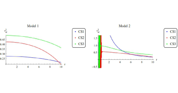
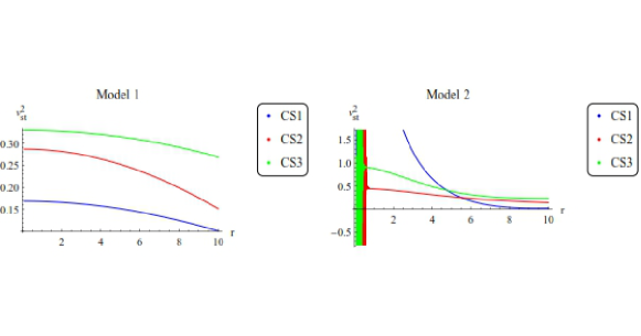
We plotted some graphs by using Eqs.(4.2)-(4.3) and (5.3)-(5.5) along with Table 1. One can clearly see from the Figures (11) and (11) that $v_{sr}^{2}$ and $v_{st}^{2}$ are within the stability range for all three observed compact stellar structures. Furthermore, Figure (13) shows the stability modes like

$$0<|v_{st}^{2}-v_{sr}^{2}|<1.$$

This indicate that our compact spherical geometries are within the stability bounds even in the presence of extra degrees of freedom coming from (4.2) and (4.3) $f(R,T)$ models.

Figure 12: Change in $v_{st}^{2}-v_{sr}^{2}$ versus $r(km)$ of CS1, CS2 and CS3.

Figure 13: Change in $\Delta$ versus $r$.

5.5 The Measurement of Anisotropy

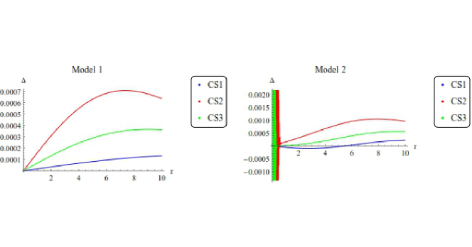
The extent of anisotropicity as well as its magnitude within a local anisotropic fluid distributions can be defined as

$$\Delta \equiv\frac{2}{r}({P_{t}}-{P_{r}}).$$

Using Eqs.(2.8)-(2.10), we can write $\Delta$ as

$$\Delta =\frac{2\exp(-Ar^{2})}{r^{3}(1+\epsilon)}[\{\exp(Ar^{2})-(1+Ar^{2}-Br^{2})(1+Br^{2})\}fi^{\prime}+r\{-(1+Ar^{2})$$

$$\times R^{\prime}fi^{\prime\prime}+rfi^{\prime\prime}R^{\prime\prime}+rR^{\prime 2}fi^{\prime\prime\prime}\}].$$

The above equation contains $fi$ terms. We use the two different viable $fi$ models from Eqs.(4.2)-(4.3) and get the three different equations, each incorporating a particular $f(R,T)$ model corrections. After using observational results of the compact stars given in Table 1, we terminated with six set of equations. We check the behavior of anisotropy in the degrees of anisotropicity in the background of relativistic compact objects, by plotting these equations. It can be seen from the plot shown in Figure (13) that the $\Delta$ is remained greater than zero for all the three relativistic compact stellar structures which resulting that the influence of radial pressure, $P_{r}$ is lesser than that of transverse pressure, $P_{t}$. This outward directed measure of anisotropy for these two viable models.

6 Summary

As the universe is accelerating, this ground reality attracts researchers towards the extension of GR and modified theories of gravity. The first modification to GR gives birth to $f(R)$ gravity, which provides a good attention while the extension of this modification gives rise to $f(R,T)$ gravity and attain much attentions because of some quantum effects arising in the theory. These modifications appear in the field of low energy action for effective quantum gravity theory.

In this work, we study the anisotropic relativistic compact stellar objects with static and spherical structures. For this purpose, we consider the relativistic compact stellar objects whose interior geometry is based on anisotropy in $f(R,T)$ gravity. Krori and Barua [82] proposed the relativistic interiors of stellar bodies through specific metric combnations. With these techniques, we connect this interior geometry with the exterior Schwarzschild geometry and find the constant (in term of mass and radius) of interior metric over the boundary. After this, we used some observational data from which we find the numerical values of these constants. Then we put these numerical values in our calculations and plots our results.

In this paper, we have used BK solution, according to which $a(r)=Br^{2}+C$ and $b(r)=Ar^{2}$, where $A,~{}B$ and $C$ are the three constant numbers which can be evaluated depending on several physical requirements. Such solutions [82] are claimed to be singularity-free for the static spherical systems in the background of GR. Furthermore, this solution is asserted to be regular everywhere and the matter variables, like mass density, pressure etc are finite all over within the relativistic spherical system.

It is of our interest to check the outcomes and the predictions of one of the extended gravities, i.e., $f(R,T)$ theory regarding the existence and stability of spherical stars. Therefore, we have explored the modified version of the TOV equation in the realm of couple of $f(R,T)$ models. Figure 9 states that for the particular choices of $f(R,T)$ model parameters, there exists some eras under which system could attain equilibrium condition by keeping all the forces sum to be zero. It is worthy to mention that usual GR forces are being modified due to $f(R,T)$ models, thus producing some extra effects in the forces $F_{g},~{}F_{h}$ and $F_{a}$. The stability of our compact stars not only depends upon KB-solution but also on the choices of parameters involved in $f(R,T)$ models mentioned in Eqs.(4.2) and (4.3). The difference of the squares of sound speeds, i.e, $v_{st}^{2}-v_{sr}^{2}$ has been found to be within $[0,1]$, thus describing our relativistic stars to be in stable window with certain values of parameters involved in the corresponding $f(R,T)$ models.

The energy density remains positive and maximum at the core of compact stars. Energy conditions holds for all these three compact stars and the radial as well as the transverse equation of state parameter are in a usual range i.g. $0<\omega_{i}<1$, here $i=r,t$. This indicate that the interior structures of these relativistic compacts stellar objects are composed of normal ordinary matter. For all case, we find the anisotropy directed outward, e.g., $p_{t}>p_{r}$ or $\Delta>0$. Similarly, the transverse as well as the radial sound speed for all these compact stars are in stable limits that implies the stability of these spherical anisotropic compact bodies in the realm of $f(R,T)$ gravity.

References

- [1] S. Weinberg, Rev. Mod. Phys. 61, 1 (1989); P. J. E. Peebles and B. Ratra, Rev. Mod. Phys. 75, 559 (2003); V. Husain and B. Qureshi, Phys. Rev. Lett. 116, 061302 (2016).
- [2] D. Pietrobon, A. Balbi, and D. Marinucci, Phys. Rev. D 74, 043524 (2006); T. Giannantonio et al., Phys. Rev. D 74, 063520 (2006); A. G. Riess et al., Astrophys. J. 659, 98 (2007).
- [3] P. J. E. Peebles and B. Ratra, Rev. Mod. Phys. 75, 559 (2003); V. Sahni, AIP Conf. Proc. 782, 166 (2005); J. Phys. Conf. Ser. 31, 115 (2006).
- [4] T. Padmanabhan, Phys. Rep. 380, 235 (2003).
- [5] E. J. Copeland, M. Sami, and S. Tsujikawa, Int. J. Mod. Phys. D 15, 1753 (2006).
- [6] S. Nojiri and S. D. Odintsov, Int. J. Geom. Methods Mod. Phys. 4, 115 (2007).
- [7] S. Nojiri and S. D. Odintsov, arXiv:0801.4843; arXiv:0807.0685; T. P. Sotiriou and V. Faraoni, arXiv:0805.1726; F. S. N. Lobo, arXiv:0807.1640; S. Capozziello and M. Francaviglia, Gen. Relativ. Gravit. 40, 357 (2008).
- [8] A. Qadir, H. W. Lee, and K. Y. Kim, Int. J. Mod. Phys. D 26, 1741001 (2017).
- [9] Z. Yousaf, Eur. Phys. J. Plus 132, 71 (2017).
- [10] M. Sharif and Z. Yousaf, Z.: Astrophys. Space Sci. 355, 317 (2015); M. Z. Bhatti and Z. Yousaf, Int. J. Mod. Phys. D 26, 1750029 (2017); ibid. Int. J. Mod. Phys. D 26, 1750045 (2017); M. Z. Bhatti and Z. Yousaf, Eur. Phys. J. C 76, 219 (2016) [arXiv1604.01395 [gr-qc]].
- [11] T. Harko, F. S. N. Lobo, S. Nojiri and S. D. Odintsov, Phys. Rev. D 84, 024020 (2011); Z. Yousaf and M. Z. Bhatti, Eur. Phys. J. C 76, 267 (2016) [arXiv:1604.06271 [physics.gen-ph]]; M. Sharif and Z. Yousaf, Astrophys. Space Sci. 354, 471 (2014); Yousaf, Z., Bamba, K. and Bhatti, M. Z.: Phys. Rev. D 95, 024024 (2017) [arXiv:1701.03067 [gr-qc]].
- [12] S. Nojiri and S. D. Odintsov, Phys. Lett. B 631, 1 (2005).
- [13] S. D. Odintsov and D. Sáez-Gómez, Phys. Lett. B, 725, 437 (2013); Z. Haghani, T. Harko, F. S. N. Lobo, H. R. Sepangi and S. Shahidi, Phys. Rev. D, 88, 044023 (2013); I. Ayuso, J. B. Jiménez and Á de la Cruz-Dombriz, Phys. Rev. D, 91, 104003 (2015); Z. Yousaf, M. Z. Bhatti and U. Farwa, Class. Quantum Grav. 34, 145002 (2017).
- [14] Nojiri, S., Odintsov, S. D. and Oikonomou, V.K.: arXiv: arXiv:1705.11098 [gr-qc].
- [15] J. C. Hwang and H. Noh, Phys. Lett. B 506, 13 (2001).
- [16] S. Nojiri and S. D. Odintsov, Phys. Rev. D 68, 123512 (2003).
- [17] M. Demianski, et al., Astron. Astrophys. 454, 55 (2006).
- [18] V. Singh and C. P. Singh, Astrophys. Space Sci. 356, 153 (2015).
- [19] T. Harko, F. S. N. Lobo, S. Nojiri and S.D. Odintsov, Phys. Rev. D 84, 024020 (2011).
- [20] S. Capozziello and V. Faraoni, Beyond Einstein Gravity (Springer, Dordrecht, 2010).
- [21] S. Capozziello and M. De Laurentis, Phys. Rept. 509, 167 (2011) [arXiv:1108.6266 [gr-qc]].
- [22] K. Bamba, S. Capozziello, S. Nojiri and S. D. Odintsov, Astrophys. Space Sci. 342, 155 (2012) [arXiv:1205.3421 [gr-qc]].
- [23] K. Koyama,Rep. Prog. Phys. 79, 046902 (2016) [arXiv:1504.04623 [astro-ph.CO]].
- [24] Á. de la Cruz-Dombriz and D. Sáez-Gómez, Entropy 14, 1717 (2012) [arXiv:1207.2663 [gr-qc]].
- [25] K. Bamba, S. Nojiri and S. D. Odintsov, arXiv:1302.4831 [gr-qc].
- [26] K. Bamba and S. D. Odintsov, arXiv:1402.7114 [hep-th]; Symmetry 7, 220 (2015) [arXiv:1503.00442 [hep-th]].
- [27] Z. Yousaf, K. Bamba and M. Z. Bhatti, Phys. Rev. D 93, 064059 (2016) [arXiv1603.03175 [gr-qc]].
- [28] Z. Yousaf, K. Bamba and M. Z. Bhatti, Phys. Rev. D 93, 124048 (2016) [arXiv:1606.00147 [gr-qc]].
- [29] S. Nojiri, and S. D. Odintsov, eConf C 0602061, 06 (2006); Int. J. Geom. Meth. Mod. Phys. 4, 115 (2007) [hep-th/0601213].
- [30] S. Nojiri, and S. D. Odintsov, arXiv:0801.4843 [astro-ph] (2008).
- [31] S. Nojiri, and S. D. Odintsov, arXiv:0807.0685 [hep-th] (2008).
- [32] Sotiriou, T. P. and Faraoni, V.: Rev. Mod. Phys. 82, 451 (2010).
- [33] P. H. R. S. Moraes, Astrophys. Space Sci. 352, 273 (2014).
- [34] P. H. R. S. Moraes, Eur. Phys. J. C 75, 168 (2015); P. H. R. S. Moraes, Int. J. Theor. Phys. 55, 1307 (2016).
- [35] C. P. Singh and P. Kumar, Eur. Phys. J. C 74, 11 (2014).
- [36] H. Shabani and M. Farhoudi, Phys. Rev. D 90, 044031 (2014).
- [37] D. R. K. Reddy and R. S. Kumar, Astrophys. Space Sci. 344, 253 (2013).
- [38] P. Kumar and C. P. Singh, Astrophys. Space Sci. 357, 120 (2015).
- [39] M. Sharif and Z. Yousaf, Astrophys. Space Sci. 354, 471 (2014).
- [40] Z. Yousaf, M. Ilyas and M. Z. Bhatti, Eur. Phys. J. Plus 132, 268 (2017).
- [41] Z. Yousaf, M. Ilyas and M. Z. Bhatti, Mod. Phys. lett. A 32, 1750163 (2017).
- [42] M. Z. Bhatti and Z. Yousaf, Ann. Phys. DOI: 10.1016/j.aop.2017.10.014 [arXiv:1701.08646 [physics.gen-ph]].
- [43] A. Alhamzawi and R. Alhamzawi, Int. J. Mod. Phys. D 25, 1650020 (2015).
- [44] P. H. R. S. Moraes, J. D. V. Arbañil and M. Malheiro, J. Cosmol. Astropart. Phys. 06, 005 (2016).
- [45] M. J. S. Houndjo, Int. J. Mod. Phys. D 21, 1250003 (2012).
- [46] E. H. Baffou, A. V. Kpadonou, M. E. Rodrigues, M. J. S. Houndjo and J. Tossa, Astrophys. Space Sci. 356, 173 (2014).
- [47] K. Bamba, S. Capozziello, S. Nojiri and S. D. Odintsov, Astrophys. Space Sci. 342, 155 (2012).
- [48] R. Durrer and R. Maartens, arXiv:0811.4132 [astro-ph].
- [49] S. Capozziello, M. De Laurentis, I. De Martino, M. Formisano and S. D. Odintsov, Phys. Rev. D 85 044022, (2012) [arXiv: 1112.0761].
- [50] S. Capozziello, M. De Laurentis, S. D. Odintsov and A. Stabile Phys. Rev. D 83, 064004 (2011) [arXiv: 1101.0219 [gr-qc]].
- [51] K. Bamba, S. Nojiri and S. D. Odintsov, Phys. Lett. B 698, 451 (2011) [arXiv: 1101.2820].
- [52] A. Das, F. Rahaman, B. K. Guha and S. Ray, Astrophys. Space Sci. 358, 36 (2015).
- [53] K. Bamba, M. Ilyas, M. Z. Bhatti and Z. Yousaf, Gen. Relativ. Gravit. 49, 112 (2017) [arXiv:1707.07386 [gr-qc]].
- [54] M. Sharif and Z. Yousaf, Eur. Phys. J. C 75, 58 (2015); M. Z. Bhatti, Z. Yousaf and S. Hanif, Mod. Phys. Lett. A 32, 1750042 (2017); Phys. Dark Universe 75, 58 (2017).
- [55] M. Sharif and Z. Yousaf, Eur. Phys. J. C 75, 194 (2015) [arXiv:1504.04367v1 [gr-qc]]; M. Sharif and Z. Yousaf, Astrophys. Space Sci. 355, 317 (2015); Z. Yousaf, M. Z. Bhatti and U. Farwa, Mon. Not. R. Astron. Soc. 464, 4509 (2017); M. Z. Bhatti, Eur. Phys. J. Plus 131, 428 (2016); Z. Yousaf, Eur. Phys. J. Plus 132, 71 (2017).
- [56] M. Sharif and Z. Yousaf, Astrophys. Space Sci. 357, 49 (2015); Z. Yousaf and M. Z. Bhatti, Eur. Phys. J. C 76, 267 (2016) [arXiv:1604.06271 [physics.gen-ph]]; Z. Yousaf, M. Z. Bhatti and U. Farwa, Class. Quantum Grav. 34, 145002 (2017) [arXiv:1709.04365 [gr-qc]]; Z. Yousaf, Eur. Phys. J. Plus 132, 276 (2017).
- [57] P. K. Sahoo, P. Sahoo, B. K. Bishi, Int. J. Geom. Meth. Mod. Phys, 14, 1750097 (2017) [arXiv:1702.02469 [gr-qc]]; P. H. R. S. Moraes and P. K. Sahoo, Eur. Phys. J. C 77, 480 (2017); P. K. Sahoo, P. Sahoo, B. K. Bishi and S. Aygün, arXiv:1707.00979 [gr-qc].
- [58] P. H. R. S. Moraes, J. D. V. Arbañil and M. Malheiro, J. Cosmol. Astropart. Phys. 06, 005 (2016).
- [59] C. W. Misner, K. S. Thorne and J. A. Wheeler, Mon. Not. R. Astron. Soc. 68, 164 (1974).
- [60] T. Chiba, J. Cosmol. Astropart. Phys. 03, 008 (2005).
- [61] S. Arapoglu, C. Deliduman and K. Y. Eksi, J. Cosmol. Astropart. Phys. 07 , 020 (2011).
- [62] A. V. Astashenok, S. Capozziello and S. D. Odintsov, Phys. Rev. D 89, 103509 (2014).
- [63] A. V. Astashenok, S. Capozziello and S. D. Odintsov, J. Cosmol. Astropart. Phys. 01, 001 (2015)
- [64] K. V. Staykov, D. D. Doneva and S. S. Yazadjiev, Eur. Phys. J. C 75, 607 (2015)
- [65] S. Capozziello, M. De Laurentis, R. Farinelli and S. D. Odintsov, Phys. Rev. D 93 023501 (2016).
- [66] M. F. Shamir and M. Ahmad, Eur. Phys. J. C 77, 674 (2017).
- [67] S. S. Yazadjiev, D. D. Doneva, K. D. Kokkotas, Phys. Rev. D 91, 084018 (2015).
- [68] K. S. Virbhadra, D. Narasimha, and S. M. Chitre, Astron. Astrophys. 337, 1 (1998); K. S. Virbhadra and G. F. R. Ellis, Phys. Rev. D 65, 103004 (2002).
- [69] K. S. Virbhadra, Phys. Rev. D 79, 083004 (2009).
- [70] M. Sharif and Z. Yousaf, Gen. Relativ. Gravit. 47, 48 (2015).
- [71] M. Z. Bhatti, Z. Yousaf and M. Ilyas, Eur. Phys. J. C, Eur. Phys. J. C 77, 690 (2017) [arXiv1709.06892 [gr-qc]]
- [72] Z. Yousaf, M. Sharif, M. Ilyas and M. Z. Bhatti, Eur. Phys. J. C 77, 691 (2017) [arXiv1710.05717 [gr-qc]].
- [73] B. M. Schaefer and K. Koyama, Mon. Not. R. Astron. Soc. 385, 411 (2008).
- [74] S. Capozziello, M. De Laurentis, S. D. Odintsov, and A. Stabile, Phys. Rev. D 83, 064004 (2011).
- [75] J. A. R. Cembranos, Á. de la Cruz-Dombriz and B. M. Núñez, J. Cosmol. Astropart. Phys. 04, 021 (2012)
- [76] A. V. Astashenok, S. Capozziello and S. D. Odintsov, J. Cosmol. Astropart. Phys. 12, 040 (2013).
- [77] Z. Yousaf and M. Z. Bhatti, Mon. Not. R. Astron. Soc. 458, 1785 (2016) [arXiv:1612.02325 [physics.gen-ph]].
- [78] M. A. Resco, Á. de la Cruz-Dombriz, F. J. L. Estrada and V. Z. Castrillo, Phys, Dark Universe 13, 147 (2016).
- [79] K. Bamba, M. Ilyas, M. Z. Bhatti and Z. Yousaf, Gen. Relativ. Gravit. 49, 112 (2017) [arXiv:1707.07386 [gr-qc]].
- [80] G. Abbas, S. Nazeer and M. A. Meraj, Astrophys Space Sci 354, 449 (2014).
- [81] E. Egeland, Compact Stars (Trondheim, Norway, 2007).
- [82] K. D. Krori and J. Barua, J. Phys. A: Math. Gen. 8, 508 (1975).
- [83] H. A. Buchdahl, Phys. Rev. 116, 1027 (1959); H. A. Buchdahl, Astrophys. J., 146, 275 (1966).
- [84] S. S.Yazadjiev, D. D. Doneva, K. D. Kokkotas and K. V. Staykov, J. Cosmol. Astropart. Phys. 06, 003 (2014).
- [85] G. Lambiase, Phys. Rev. D 90, 064050 (2014).
- [86] A. A. Starobinsky, J. Exp. Theor. Phys. Lett. 86, 157 (2007); S. Tsujikawa, Phys. Rev. D 77, 023507 (2008).
- [87] L. Herrera, Phys. Lett. A 165, 206 (1992).
- [88] B. M. Schaefer and K. Koyama, Mon. Not. R. Astron. Soc. 385, 411 (2008).
- [89] S. Capozziello, M. De Laurentis, S. D. Odintsov, and A. Stabile, Phys. Rev. D 83, 064004 (2011).
- [90] J. A. R. Cembranos, Á. de la Cruz-Dombriz and B. M. Núñez, J. Cosmol. Astropart. Phys. 04, 021 (2012)
- [91] A. V. Astashenok, S. Capozziello and S. D. Odintsov, J. Cosmol. Astropart. Phys. 12, 040 (2013).
- [92] M. A. Resco, Á. de la Cruz-Dombriz, F. J. L. Estrada and V. Z. Castrillo, Phys, Dark Universe 13, 147 (2016).
- [93] K. Bamba, M. Ilyas, M. Z. Bhatti and Z. Yousaf, Gen. Relativ. Gravit. 49, 112 (2017) [arXiv:1707.07386 [gr-qc]].
- [94] C. W. Misner and D. Sharp, Phys. Rev. 136, B571 (1964).
- [95] Darmois, G.: Memorial des Sciences Mathematiques (Gautheir-Villars, 1927) Fasc. 25.