New classes of solutions in the Coupled $\cal{PT}$ Symmetric Nonlocal Nonlinear Schrödinger Equations with Four Wave Mixing

Abstract

We investigate generalized nonlocal coupled nonlinear Schorödinger equation containing Self-Phase Modulation, Cross-Phase Modulation and Four Wave Mixing involving nonlocal interaction. By means of Darboux transformation we obtained a family of exact breathers and solitons including the Peregrine soliton, Kuznetsov-Ma breather, Akhmediev breather along with all kinds of soliton-soliton and breather-soltion interactions. We analyze and emphasize the impact of the four-wave mixing on the nature and interaction of the solutions. We found that the presence of Four Wave Mixing converts a two-soliton solution into an Akhmediev breather. In particular, the inclusion of Four Wave Mixing results in the generation of a new solutions which is spatially and temporally periodic called “Soliton (Breather) lattice”.

1 Introduction

Since the invention of the laser, optical solitons [1] have played an important role in nonlinear physics. The optical soliton in fibres is probably the best studied form of solitons because of its remarkable behavior that agrees well with theoretical predictions and its potential as optical information carrier. The propagation of optical pulses through optical birefringent fibres is described by the celebrated Manakov model of the following form [2],

$$\textit{i}q_{1t} + q_{1xx}+2\left(g_{11}|q_{1}|^{2}+g_{12}|q_{2}|^{2}\right)q_{1}=0,$$ (1a)

$$\textit{i}q_{2t} + q_{2xx}+2\left(g_{21}|q_{1}|^{2}+g_{22}|q_{2}|^{2}\right)q_{2}=0,$$ (1b)

where, $q_{1}$ and $q_{2}$ are wave envelopes, $x$, $t$ are space and time variables and $i$ is the imaginary unit. The interaction coefficients $g_{11}$ and $g_{22}$ correspond to the Self-Phase Modulation (SPM) and $g_{12}$ and $g_{21}$ represent the Cross-Phase Modulation (XPM) [3]. Eq. (1) has been shown to be integrable if either (i) $g_{11}$ = $g_{12}$ =$g_{21}$ =$g_{22}$ or (ii) $g_{11}$ = $g_{21}$ =-$g_{12}$ =-$g_{22}$ [4]. The first choice corresponds to Manakov model [5] while the second choice represents the modified Manakov model [6]. The above coupled nonlinear Schrödinger equation (CNLSE) involving local nonlinear interactions has been extensively studied in diverse fields such as nonlinear optics [7], bio-physics [8], finance [9] and oceanographic studies [10] etc.

After the discovery of new integrable model named “nonlocal integrable NLSE ” by Ablowitz and Mussilimani [11], the integrable models involving nonlocal interactions have attracted considerable attention. In ref.[11] Ablowitz et al., introduced the model of the following form

$$\textit{i}q_{t}(x,t)=q_{xx}(x,t)+2\,g\,q(x,t)q^{\ast}(-x,t)\,q(x,t).$$ (2)

This equation (2) is $\cal{PT}$ symmetric in the sense that the equation brings a self-induced potential of the form $V(x,t)=q(x,t)q^{\ast}(-x,t)$ and satisfies the $\cal{PT}$ symmetric condition $V(x,t)=V^{\ast}(-x,t)$. It is nonlocal in the sense that the evolution of the field at transverse coordinate $x$ always requires the information from the opposite point $-x$ [11]. Interestingly, in this study Ablowitz et al., have shown the new model given by Eq. (2) to be fully integrable since it possesses linear Lax pair and infinite number of conserved quantities. Unlike the integrable model considering local nonlinear interaction, the above new integrable model involving nonlocal interactions is very rich in the sense of giving rise to new results and possessing some new behaviors, e.g., it simultaneously admits both the bright and dark soliton solutions for the same nonlinearity [12]. In addition, several studies involving nonlocal $\cal{PT}$ symmetric optics can lead to alternative classes of optical structures and devices with unique properties. These include the effect of nonlinearity on beam dynamics in $\cal{PT}$ symmetric potential [13], solitons in dual-core waveguides [14, 15], and Bragg solitons in $\cal{PT}$ symmetric potentials [16]. Finally $\cal{PT}$ symmetric concepts have also been studied in plasmonics [17], optical metamaterials [18, 19] and coherent atomic medium [20].

Four wave mixing (FWM) is one of the most important nonlinear phenomena having practical applications, particularly in nonlinear optics [3, 21] such as optical processing [22], real time holography [23], Phase conjugate optics [24], measurement of atomic energy structures and decay rates [25]. In addition, the FWM phenomenon also has wider applications in communication networks to create new waves and reduce loss in the signals. The easiest way to obtain FWM in a fibre is to propagate two waves at angular frequencies $\omega_{1}$ and $\omega_{2}$ that will create new frequencies $\omega_{3}$ and $\omega_{4}$ such as $\omega_{1}+\omega_{2}$ = $\omega_{3}+\omega_{4}$. On the other hand, the coupled version of the above nonlocal equation, Eq. (2), has also received considerable attention and its dynamics has also been studied [26]. Unlike the classical Manakov model, this coupled nonlocal equation admits all classes of solitonic solutions for the same nonlinearity and it does so only in the presence of nonlocal interactions.

Motivated by the above results involving nonlocality and its unique behaviors with wide range of applications in diverse fields, we consider the model of coupled NLSE with nonlocal SPM and XPM along with FWM parameter. The latter is particularly important since FWM is an essential feature of optical solitons while carrying signals through the birefringent fibre under suitable conditions. The details of the model are given in detail in the next section.

We employ the powerful method of Darboux transformation to find the new solutions of the present model. We found that i) the inclusion of FWM in the nonlocal NLSE leads to conversion of a soliton-soliton pair , namely Bright(B)-Dark(D), B-B, or D-D, into an Akhmediev breather, and ii) the manipulation of FWM parameters gives a chance to observe a new solution of a breather-soliton pair. In addition, we also find some interesting exact solutions including the Peregrine, Kuznetsov-Ma breather, Akhmediev breather, and a breathing travelling solitonic wave, we called it as Soliton (Breather) lattice.

The plan of the paper is as follows. In section II, we present the mathematical (integrable) model governing the dynamics of nonlocal $\cal{PT}$ symmetric coupled NLSE with nonlocal FWM. In section III, we present the corresponding Lax pair and then derive the explicit soliton solution for zero and non-zero seed. In section IV, we investigate the impact of FWM in nonlocal CNLSE. In section V, we derive the special cases of the Peregrine, Ma, Akhmediev breathers. The results are then summarized in section VI.

2 Model Equations

We consider the generalized $\cal{PT}$ symmetric nonlocal NLSE with nonlocal SPM, XPM and FWM of the following form,

$$\textit{i}\,\frac{\partial q_{1}(x,t)}{\partial t}+\frac{\partial^{2}q_{1}(x,t)}{\partial x^{2}}\,+\Big{[} a\,q_{1}(x,t)\,q_{1}^{\ast}(-x,t)\,+\,b\,q_{1}(x,t)\,q_{2}^{\ast}(-x,t)\,$$

$$+\,c\,q_{2}(x,t)q_{2}^{\ast}(-x,t)\,+\,d\,q_{1}^{\ast}(-x,t)\,q_{2}(x,t)\Big{]}q_{1}(x,t)=0,$$ (3a)

$$\textit{i}\,\frac{\partial q_{2}(x,t)}{\partial t}+\frac{\partial^{2}q_{2}(x,t)}{\partial x^{2}}\,+\Big{[} a\,q_{1}(x,t)\,q_{1}^{\ast}(-x,t)\,+\,b\,q_{1}(x,t)\,q_{2}^{\ast}(-x,t)\,$$

$$+\,c\,q_{2}(x,t)q_{2}^{\ast}(-x,t)\,+\,d\,q_{1}^{\ast}(-x,t)\,q_{2}(x,t)\Big{]}q_{2}(x,t)=0,$$ (3b)

where, $q_{1,2}(x,t)$ are two complex field variables and the coefficients $a,\,c$ correspond to the nonlocal SPM and XPM while $b,\;d$ represent the nonlocal FWM terms. The subscripts $x,t$ denote the derivatives with respect to the spatial and temporal variables. For the sack of simplicity, the local interactions in the above coupled NLSE $[|q_{1}|^{2}+|q_{2}|^{2}]q_{1}$ and $[|q_{1}|^{2}+|q_{2}|^{2}]q_{2}$ is replaced by their $\cal{PT}$ symmetric counterparts, namely, $[q_{1}q_{1}^{\ast}(-x,t)+q_{2}q_{2}^{\ast}(-x,t)]q_{1}$ and $[q_{1}q_{1}^{\ast}(-x,t)+q_{2}q_{2}^{\ast}(-x,t)]q_{2}$, along with nonlocal FWM interactions to obtain generalized coupled nonlocal NLSE given by Eqs. (3) by using the transformation given by Eqs. (6).

3 Lax-Pair and Darboux transformation

3.1 Lax-Pair

Applying the Darboux transformation (DT) [27] method on nonlocal generalized CNLS equation requires finding a linear system of equations for an auxiliary fields ${\bf\Phi}(x,t)$. The linear system is usually written in compact form in terms of the pair of matrices as follows

$${\bf\Phi}_{x} = {\bf U\Phi},$$ (4a)

$${\bf\Phi}_{t} = {\bf V\Phi},$$ (4b)

where, ${\bf U}$ and ${\bf V}$, known as the Lax pair, are functionals of the solutions of the model equations. The consistency condition of the linear system ${\bf\Phi}_{xt}={\bf\Phi}_{tx}$ must be equivalent to the model equation under consideration.

We find the following linear system which corresponds to the class of generalized nonlocal coupled NLS with cross-phase and self-phase modulation,

$${\bf\Phi}_{x} ={\bf U}_{0}\,{\bf\Phi}+{\bf U}_{1}\,{\bf\Phi}\,{\bf\Lambda}$$ (5a)

$${\bf\Phi}_{t} ={\bf V}_{0}\,{\bf\Phi}+{\bf V}_{1}\,{\bf\Phi}\,{\bf\Lambda}+{\bf V}_{2}\,{\bf\Phi}\,{\bf\Lambda}^{2}$$ (5b)

where,

$${\bf\Phi}=\begin{pmatrix}\psi_{1}(x,t)&\psi_{2}(x,t)&\psi_{3}(x,t)\\ \\ \phi_{1}(x,t)&\phi_{2}(x,t)&\phi_{3}(x,t)\\ \\ \chi_{1}(x,t)&\chi_{2}(x,t)&\chi_{3}(x,t)\end{pmatrix},\;\;\;{\bf U}_{0}=\begin{pmatrix}0&-1&0\\ \\ 0&0&-1\end{pmatrix},$$

$${\bf\Lambda} =\begin{pmatrix}\lambda_{1}&0&0\\ \\ 0&\lambda_{2}&0\\ \\ 0&0&\lambda_{3}\end{pmatrix},\;\;\;{\bf V}_{0}=\frac{\mathrm{i}}{2}\begin{pmatrix}q_{1}(x,t)r_{1}(x,t)+q_{2}(x,t)r_{2}(x,t)&q_{1x}(x,t)&q_{2x}(x,t)\\ \\ r_{1x}(x,t)&-q_{1}(x,t)r_{1}(x,t)&-q_{2}(x,t)r_{1}(x,t)\\ \\ r_{2x}(x,t)&-q_{1}(x,t)r_{2}(x,t)&-q_{2}(x,t)r_{2}(x,t)\end{pmatrix},$$

$${\bf V}_{1} =\begin{pmatrix}0&-q_{1}(x,t)&-q_{2}(x,t)\\ \\ r_{1}(x,t)&0&0\\ \\ r_{2}(x,t)&0&0\end{pmatrix},\;\;\;{\bf V}_{2}=\mathrm{i}\begin{pmatrix}1&0&0\\ \\ 0&-1&0\\ \\ 0&0&-1\end{pmatrix},$$

along with the transformation on the complex conjugates

$$r_{1}(x,t) =aq_{1}^{\ast}(-x,t)+bq_{2}^{\ast}(-x,t)$$ (6a)

$$r_{2}(x,t) =dq_{1}^{\ast}(-x,t)+cq_{2}^{\ast}(-x,t)$$ (6b)

where $\lambda_{1,2,3}$ is the spectral parameter. The consistency condition ${\bf\Phi}_{xt}={\bf\Phi}_{tx}$ leads to ${\bf U}_{t}-{\bf V}_{x}+[{\bf U},{\bf V}]={\bf 0}$ which should generate the model equation (3).

Using the DT we have solved the above model equations using trivial (zero) seed to obtain a single soliton solution and non-zero seed to obtain the higher order soliton solutions.

3.2 Darboux Transformation with zero seed: Single soliton solution

Considering the following version of DT [27]

$${\bf\Phi[{\rm 1}]}={\bf\Phi\Lambda-\sigma\Phi},$$ (7)

where, ${\bf\Phi}[1]$ is the transformed field and $\sigma=\Phi_{0}\,\Lambda\,\Phi_{0}^{-1}$ and ${\bf\Phi_{0}}$ is a known solution of the linear system (5), we apply the DT on the linear system given by Eqs. (4), and the stipulation that the transformed linear system be covariant with the original one requires

$${\bf U_{0}}[1]={\bf U_{0}}+[{\bf U_{1}},{\bf\sigma}].$$ (8)

The new solution to the nonlinear equations given by, Eqs. (3), in terms of the seed solution is obtained from the last equation.

Following this procedure, we derive the simple first order soliton solution,

$$q_{1}(x,t) = \frac{A\,c\,C_{1}\,e^{-(2\,\mathrm{i}\,t+2\,x})}{2\,c\,C_{2}\,e^{2(2\,\mathrm{i}\,t+2\,x)}+\,C_{3}(\delta_{1}+\sqrt{\delta_{2}})\,e^{2(2\,\mathrm{i}\,t+2\,x)}}$$ (9a)

$$q_{2}(x,t) = \frac{A\,c\,C_{1}\,(\delta_{1}\,+\sqrt{\delta_{2}})\,e^{-(2\mathrm{i}\,t+2\,x)}}{2\,c\,C_{2}\,e^{2(2\mathrm{i}\,t\,+\,2\,x)}+C_{3}\,(\delta_{1}\,+\sqrt{\delta_{2}})\,e^{2(2\,\mathrm{i}\,t\,+2\,x)}}$$ (9b)

with $A$ a complex constant and $C_{1,2,3}$ are arbitrary real constants with, $\delta_{1}=-b-d$, $\delta_{2}=b^{2}\,-4\,a\,c\,+2\,b\,d\,+\,d^{2}$. It should be noted that in order to obtain such a localized solution we have set the following values to the spectral parameters: $\lambda_{1}=\lambda_{3}=-\textit{i}$ and $\lambda_{2}=\textit{i}\lambda_{3}$.

We observe from Eqs. (9) that the nonlocal FWM alongwith nonlocal SPM and XPM merely varies the amplitudes of the solutions of the nonlocal CNLSE. Hence, we focus on the impact of FWM alongwith SPM and XPM with nontrivial seed in the next section.

3.3 Darboux Transformation with Constant-Wave seed: Breathers and soliton pairs

Here we apply the DT using a nonzero seed, namely the so-called Constant-Wave (CW) solution

$$q_{1}(x,t) = \alpha_{1}\textit{e}^{\textit{i}\,\phi\,t},$$ (10a)

$$q_{2}(x,t) = \alpha_{2}\textit{e}^{\textit{i}\,\phi\,t},$$ (10b)

where $\phi=a\alpha_{1}^{2}+d\alpha_{2}^{2}+2b\alpha_{1}\alpha_{2}$.

The derivation of the new solution is lengthy but straightforward. We show here only the final results. The general soliton solutions, in this case, have the following form

$$q_{k}[1]=\alpha_{k}\left[1+\frac{{\displaystyle\sum_{l=1}^{2}\sum_{m=1}^{2}\frac{c_{1,l}^{*}c_{1,m}{\rm e}^{\theta_{1,l}^{*}(-x,t)+\theta_{1,m}(x,t)}}{\xi_{1,m}}+c_{1,3}\alpha_{k}\sum_{l=1}^{2}c_{1,l}^{*}{\rm e}^{\theta_{1,l}^{*}(-x,t)}}}{{\displaystyle-\sum_{l=1}^{2}\sum_{m=1}^{2}\frac{c_{1,l}^{*}c_{1,m}{\rm e}^{\theta_{1,l}^{*}(-x,t)+\theta_{1,m}(x,t)}}{\xi_{1,l}^{*}+\xi_{1,m}}+\frac{|c_{1,3}|^{2}B}{2(\lambda_{1}^{*}+\lambda_{1})}}}\right]{\rm e}^{{\rm i}\phi t},$$ (11)

where

$$\theta_{i,1}(x,t) = {\rm i}\xi_{i,1}\left(x+\frac{1}{2}\xi_{i,1}t\right),\,\,\theta_{i,2}(x,t)={\rm i}\xi_{i,2}\left(x+\frac{1}{2}\xi_{i,2}t\right),$$ (12a)

$$\beta_{1} = -(b\alpha_{{1}}+d\alpha_{{2}}-{\rm i}c\alpha_{{1}}),\,\,\beta_{2}=a\alpha_{{1}}+b\alpha_{{2}}+{\rm i}c\alpha_{{2}},$$ (12b)

$$\xi_{i,1} = \lambda_{i}+\sqrt{\phi+\lambda_{i}^{2}},\,\,\xi_{i,2}=\lambda_{i}-\sqrt{\phi+\lambda_{i}^{2}}.$$ (12c)

with $B=a|\beta_{1}|^{2}+d|\beta_{2}|^{2}+(b+{\rm i}c)\beta_{1}\beta_{2}^{*}+(b-{\rm i}c)\beta_{1}^{*}\beta_{2}$.
This solution corresponds to a family of solitonic solutions including breathers. Each member of the family of solutions is obtained for specific values of the parameters. In the following, we present a detailed analysis of the nature and dynamics of these solutions.

4 Impact of FWM on solutions of the nonlocal coupled NLSE

In this section, we show the effect of FWM on the solutions of the nonlocal CNLSE. In Sec. 4.1, we show how FWM converts a two-soliton pair into an Akhmediev breather. In Sec. 5, we show that FWM supports new family of solutions such as a pair of breather and a soliton and a breathing solitary wave, in addition to the previously all known breathers including Akmediev and Kuznetsov-Ma breathers and the Peregrine soliton.

4.1 Two soliton solution

With no FWM, the higher order solitonic solutions are shown to be a pair of B-B, D-D, or B-D solitons [28]. For completeness, and to show the effect of FWM, we present these solutions here, which may be obtained from Eq. (11) by choosing $c_{1,3}=0$ and $c_{1,1}c_{1,2}\neq 0$, rendering Eq.(11) into the following compact form:

$$q_{k}[1]=\alpha_{k}\left[\frac{\cosh(\varphi_{1r})\cosh(A-2{\rm i}\varphi_{1i})+\cos(\varphi_{1i})\cosh(B+2\varphi_{1r})}{\cosh(\varphi_{1r})\cosh(A)+\cos(\varphi_{1i})\cosh(B)}\right]{\rm e}^{{\rm i}\phi t}$$ (13)

where

$$A = 2{\rm i}\sqrt{-\phi}\sinh(\varphi_{1r})\cos(\varphi_{1i})x+\phi\cosh(2\varphi_{1r})\sin(2\varphi_{1i})t+a_{1},$$ (14a)

$$B = 2\sqrt{-\phi}\cosh(\varphi_{1r})\sin(\varphi_{1i})x+{\rm i}\phi\sinh(2\varphi_{1r})\cos(2\varphi_{1i})t-{\rm i}b_{1},$$ (14b)

and $\exp{[(a_{1}+\varphi_{1r})+{\rm i}(b_{1}+\varphi_{1i})]}=c_{1,1}/c_{1,2}$. When $\sqrt{-\phi}<\lambda_{1}<\sqrt{\phi}$, or $\varphi_{1r}=0$, $0<\varphi_{1i}<\pi$, $b_{1}\neq(2k+1)\pi$, the solutions (13) correspond to the two-soliton solution. Along the line

$$2\sqrt{-\phi}\sin(\varphi_{1i})x=\phi\sin(2\varphi_{1i})t+a_{1}\pm\ln\left(\frac{1}{|\cos(\varphi_{1i})|}\right),\,\,t\rightarrow\mp\infty$$

the height of soliton $|q_{k}[1]|^{2}$ is

$$H_{1}=|\alpha_{k}|^{2}\left[1+\frac{2\sin\left(\varphi_{1i}\right)\sin\left(b_{1}-\varphi_{1i}\right)}{1+\cos\left(b_{{1}}\right)}\right],$$

while along the trajectory

$$2\sqrt{-\phi}\sin(\varphi_{1i})x=-\left[\phi\sin(2\varphi_{1i})t+a_{1}\right]\pm\ln\left(\frac{1}{|\cos(\varphi_{1i})|}\right),\,\,t\rightarrow\pm\infty$$

the height of soliton $|q_{k}[1]|^{2}$ is

$$H_{2}=|\alpha_{k}|^{2}\left[1-\frac{2\sin\left(\varphi_{1i}\right)\sin\left(b_{1}+\varphi_{1i}\right)}{1+\cos\left(b_{1}\right)}\right].$$

There are three different kinds of solutions: If $H_{1},H_{2}>|\alpha_{k}|^{2}$, it is two-bright (B-B) soliton. If $H_{1},H_{2}<|\alpha_{k}|^{2}$, it is two-dark (D-D) soliton. If $H_{1}>|\alpha_{k}|^{2}$, $H_{2}<|\alpha_{k}|^{2}$ ($H_{2}>|\alpha_{k}|^{2}$, $H_{1}<|\alpha_{k}|^{2}$), it is bright-dark (B-D) soliton, where $\alpha_{1},\beta_{1},a_{1},b_{1}$ are real arbitrary parameters and $H_{1,2}$ represents the heights of components $q_{1,2}$ respectively.

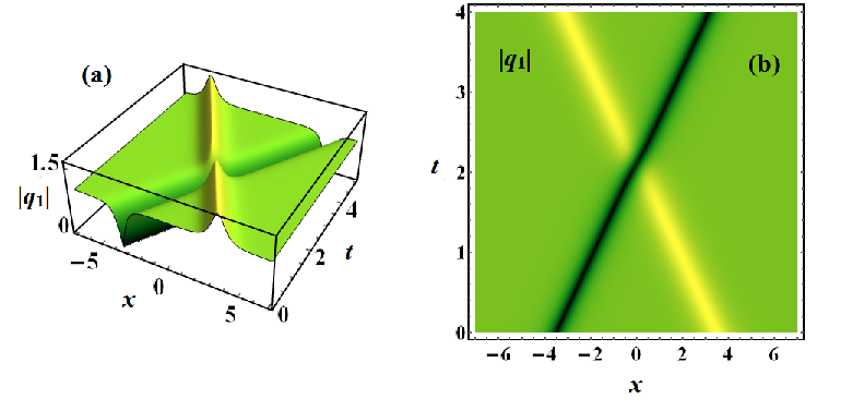
Figure 1: Bright-Dark soliton given by Eq. (13) without FWM for the parameters $\alpha_{1}=1$, $\alpha_{2}=\frac{1}{2}$,$a_{1}=8$, $b_{1}=2.5$, $a=c=-4,$ $b=d=0$, $\varphi_{1r}=0$ and $\varphi_{1i}=0.2\pi$. Similar profile occurs also for $q_{2}$ component (not shown here).

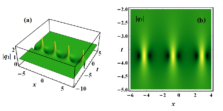
Figure 2: Impact of FWM with $b$=$d$ =5 in Eq. (13) leading to the conversion of B-D soliton of Fig. 1 into breathers. Similar Profile occurs also for $q_{2}$ component (not shown here).

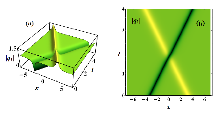
Figure 3: Impact of FWM with $b\,\neq\,d$, namely $b=-5$, $d=5$ in Eq. (13) converting the breathers in fig. 2 into a B-D Soliton. Similar Profile occurs also for $q_{2}$ component (not shown here).

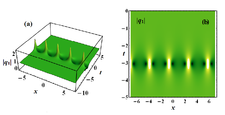
Figure 4: Retrieval of breathers from B-D solitons of Fig. 3 by changing the signs of the FWM parameters as $b=5$ and $d=-5$ given by Eq. (13). Similar Profile occurs also for $q_{2}$ component (not shown here).

4.2 Two-Soliton-Breather Conversion

The effect of the FWM on the group of B-B, D-D, and B-D solitons is predominant on the B-D soliton. Introducing FWM renders the B-D soliton into an Akhmediev breather. To understand the impact of FWM parameters $b$ and $d$ on the nonlocal coupled NLSE along with $a,\,c$, we, initially we take the B-D soliton without FWM ($b\,\&\,d=0$) alongwith $a=c$, as shown in Fig. 1. Introducing the FWM through $b$ and $d$ namely, $b=d=5$, we obtain the remarkable conversion of B-D solitons into Akhmediev breather, as shown in Fig. 2. The manipulation of $a$ and $c$ in Fig. 2 with for instance, $a$ $\textless$ $c$, $a$ $\textgreater$ $c$, or $a$ $\neq$ $c$), results only in the compression of breathers along with marginal shift towards positive or negative time scale depending upon the choice $a$ and $c$. Choosing FWM parameters $b$ and $d$ unequally such as $b$=-5, $d$=5, the breather in Fig. 2 will reverse to B-D soliton, as shown in Fig. 3. One can also retrieve the breathers, shown in Fig. 4, by interchanging the signs between $b$ and $d$ like 5 and -5, respectively, as shown in Fig. 3. The right panels are the corresponding density plots for the left panels with reduced time and space axes for better view. Another interesting impact of FWM on the nonlocal coupled NLSE is that it destroys the sensitivity to the parameter $b_{1}$. In other words, we found earlier [28] that the manipulation of the different classes of soliton solutions such as B-B, B-D, D-B, D-D solitons can be performed sensitively by the parameter $b_{1}$. The inclusion of FWM parameters in the model makes the free parameter $b_{1}$ a passive member in the group of parameters, which means the change of $b_{1}$ arbitrarily will not affect the density of the profiles shown in Fig. 1-4 in any sense, as long as FWM parameters $\neq 0$. Instead of $b_{1}$, the FWM parameters $b\,\&d$ play an active role in the conversion of any type of solitons like B-B,B-D,D-B,D-D to breathers and viceversa. We would like to add that wherever the two components exhibit similar behavior with a mere change in amplitude, we have plotted only one component ($q_{1}$) while we plot two components ($q_{1}$ and $q_{2}$) when they exhibit different behavior.

5 Family of higher order soltions with FWM

Here, we present a family of unique solitonic solutions and breathers. Some of these solutions are obtained only with FWM such as the breather-soliton solution in, Fig. 5, solitonic waves in, Fig. 6, and a new breather that is periodic in both time and space axes, as shown in Fig. 7d, which we denote here as “Soliton (Breather) lattice”.

5.1 Breather-Soliton solution

The breather-soliton solution is obtained for $c_{1,1}c_{1,2}c_{1,3}\neq 0$, $\exp{\frac{1}{2}[(a_{1}+\varphi_{1r})+{\rm i}(b_{1}+\varphi_{1i})]}=c_{1,1}$ and
$\exp{-\frac{1}{2}[(a_{1}+\varphi_{1r})+{\rm i}(b_{1}+\varphi_{1i})]}=c_{1,2}$. Since the non-singularity condition for this type of solution is very complex, we merely give a sufficient condition

$$\begin{split}\cos(\varphi_{1i})\sin(b_{1})>0,&\\ 1+\frac{|c_{1,3}|2}{4}|B|+\cos(\varphi_{1i})\cos(b_{1})>0.&\end{split}$$

In this breather-soliton solution, one dark soliton or bright soliton is replaced by the breather, as shown in Fig. 5.

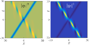
Figure 5: (color online): Breather-Soliton solution given by Eq. (13): bright soliton-breather (left) and dark soliton-breather (right) for the choice of parameters: $\alpha_{1}=1$, $\alpha_{2}=\frac{1}{4}$, $a=c=-1,$ $b=1$, $d=1$, $c_{1,1}=c_{1,2}^{-1}={\rm e}^{\frac{{\rm i}\pi}{4}}$, $c_{1,3}=1$, $\varphi_{1r}=0$ and $\varphi_{1i}=\frac{\pi}{4}$

5.2 Solitonic waves

In this section, we present a unique solitonic wave which is a travelling wave with time-dependent amplitude, as shown in Fig. 6, and is obtained by a careful choice of parameters, as given below. When we choose $|\lambda_{1}|>\sqrt{-\phi}$, $\lambda_{1}\in\mathbb{R}$, or $\varphi_{1r}\in\mathbb{R}$, $\varphi_{1i}=0$: There are three kinds of periodic solutions.

If $c_{1,3}=0$, the solution (11) can be rewritten as

$$q_{k}[1]=\alpha_{k}\left[\frac{\sinh(\varphi_{1r})\sinh(A-2{\rm i}\varphi_{1i})-\cos(\varphi_{1i})\cosh(B+2\varphi_{1r})}{\sinh(\varphi_{1r})\sinh(A)+\cos(\varphi_{1i})\cosh(B)}\right]{\rm e}^{{\rm i}\phi t}$$ (15)

where

$$A = 2{\rm i}\sqrt{\phi}\cosh(\varphi_{1r})\cos(\varphi_{1i})x-\phi\cosh(2\varphi_{1r})\sin(2\varphi_{1i})t+a_{1},$$ (16)

$$B = 2\sqrt{\phi}\sinh(\varphi_{1r})\sin(\varphi_{1i})x-{\rm i}\phi\sinh(2\varphi_{1r})\cos(2\varphi_{1i})t-{\rm i}b_{1},$$ (17)

and $\exp{[(a_{1}+\varphi_{1r})+{\rm i}(b_{1}+\varphi_{1i})]}=c_{1,1}/c_{1,2}$. Here, we consider a special case $\varphi_{1r}\in\mathbb{R}/\{0\}$, $\varphi_{1i}=0$. When $|\sinh(\varphi_{1r})\sinh(a_{1})|>1$, then one can obtain periodic solution. Similar to the defocusing case, we can obtain another periodic solution when $c_{1,3}\neq 0.$ We ignore here the analysis of the non-singularity condition since it is very complex.

If $c_{1,2}=0$, $c_{1,1}=1$, $c_{1,3}\neq 0$ and $2\cosh(\varphi_{1r})\neq{\rm e}^{\varphi_{1r}}|c_{1,3}|^{2}|B|$, or $c_{1,1}=0$ and $c_{1,2}c_{1,3}\neq 0$, then solution (11) is also a periodic solution.

We have shown periodic solution here in Fig. 6 for the choice $c_{1,1}=0$, $c_{1,2}c_{1,3}\neq 0$ given by Eq. (15).

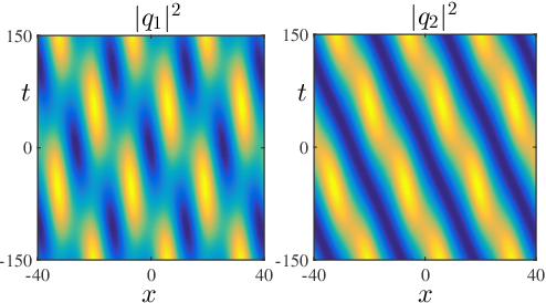
Figure 6: (color online): Periodic solutions given by Eq. (15) for the choice of parameters $\alpha_{1}=1$, $\alpha_{2}=\frac{1}{4}$, $a=c=-1,$ $b=\frac{1}{2}$, $d=\frac{1}{2}$, $c_{1,1}=0$, $c_{1,2}={\rm e}^{\frac{-{\rm i}\pi}{4}}$, $c_{1,3}=1$, $\varphi_{1r}=\mathrm{arccosh}(2)$ and $\varphi_{1i}=0$.

5.3 Breathers: Kuznetsov-Ma breather, Akhmediev breather, and Peregrine soliton

In addition to the above effect of FWM, we found that the nonlocal coupled NLSE given by Eq. (3) supports some interesting profiles such as Peregrine solitons, Kuznetsov-Ma breather, Akhmediev breathers, Space-Time breather [29]. Peregrine solitons are obtained for the choice of parameters such that the oscillatory and exponential terms in the solution given by, Eq. (15) vanish each other. This is obtained by the choice $\varphi_{1r}=0$ and $\varphi_{1i}\neq 0$, as shown in Fig. 7a. For the choice of parameter $\varphi_{1r}\neq 0$ and $\varphi_{1i}=0$, one obtains spatially localized temporally periodic Kuznetsov-Ma breather as shown in Fig. 7b. One can also obtain temporally localized and spatially periodical Akhmediev breathers as shown in Fig. 7c for the choice of parameter $\varphi_{1r}=0$ and $\varphi_{1i}=0.3\pi$. We also notice an interesting profile which is both spatially and temporally periodic which can be also viewed as a travelling breathing wave along the time axis with a phase shift. We called it as Soliton (breather) lattice, as shown in Fig. 7d. We believe that these breathers are found for the first time in the literature for the model involving nonlocal interactions with FWM.

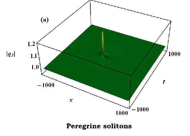
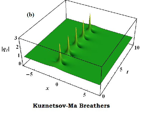
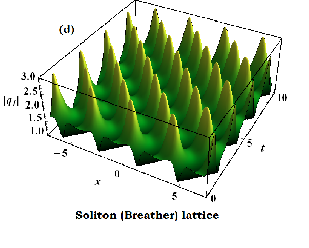
Figure 7: Different types of breathers given by Eq. (15): (a) Peregrine solitons for the choice of parameters $\alpha_{1}=1$, $\alpha_{2}=\frac{1}{2}$, $a=c=-1,$ $b=5$, $d=5$, $a_{1}=0$, $b_{1}=2.5$ $\varphi_{1r}=0$ and $\varphi_{1i}=0.00013\pi$, (b) Kuznetsov-Ma breathers for the choice of parameters $\varphi_{1r}=0.3$ and $\varphi_{1i}=0$, with $a_{1}=-1$, $b_{1}=1$ other parameters are same as in (a). (c) Akhmediev breather for the choice of parameters $a=c=-4,$ $b=5$, $d=5$, $a_{1}=-2$, $b_{1}=2.5$, $\varphi_{1r}=0$ and $\varphi_{1i}=0.3\pi$, (d) Soliton (breather) lattice for the choice of parameters $a=c=-1,$ $b=0.1$, $d=0.1$, $a_{1}=0$, $b_{1}=1$ $\varphi_{1r}=0.8$ and $\varphi_{1i}=0$.

6 Conclusion

In this paper, we investigated $\cal{PT}$ symmetric coupled nonlinear schrödinger equation with nonlocal four-wave mixing employing Darboux transformation to generate a family of exact solitonic solutions including the Peregrine soliton, Kuznetsov Ma-breather, Akhmediev breather, and a breather which is periodic in both space and time (we named it them Soliton (breather) lattice). In addition, two soliton solutions including bright-bright, dark-dark, and bright-dark turn out to be solutions of the model. We have shown that the inclusion of four-wave mixing in the nonlocal nonlinear schrödinger equation leads to conversion of bright-dark solitons into breathers. We also observe that by manipulating the four-wave mixing parameters associated with other arbitrary parameters of the system, one can observe all possible conversions between soliton-soliton interaction into breathers and vice versa. We believe that the above phenomenon occurs due to the nonlocal nature of the dynamical system with nonlocal four-wave mixing.

References

• [1] Hasegawa A, Tappert F. Transmission of stationary nonlinear optical pulses in dispersive dielectric fibers. I. Anomalous dispersion. Appl Phys Lett 1973; 23: 142.
• [2] Manakov S V. On the theory of two dimensional statioanary self-focusing of electro magnetic waves. Zh Eksp Teor Fiz 1973; 65: 505.
• [3] Agrawal G P. Nonlinear Fibre optics. New york: Academic Press; 2006.
• [4] Radha R, Vinayagam P S, Porsezian K. Rotation of the trajectories of bright solitons and realignment of intensity distribution in the coupled nonlinear SchrΓΆdinger equation. Phys Rev E 2013; 88: 032903.
• [5] Kaup D J, Malomed B A. Soliton trapping and daughter waves in the Manakov model. Phys Rev A 1993; 48: 599.
• [6] Makhankov V G, Makhaldiani N V, Pashaev O K. On the integrability and iso-otpic structure of the one dimensional Hubbard model in the long wave approximation. Phys Lett A 1981; 81: 161.
• [7] Park Q H, Shin H J. Systematic construction of vector soltions. IEEE J Quantum Electron 2002; 8: 432.
• [8] Scott A C. Launching a Davydov Soliton: I. Soliton Analysis. Phys Scr 1984; 29: No 3: 279.
• [9] Yan Z. Vector financial rogue waves. Phys Lett A 2011; 375: 4274.
• [10] Dhar A K, Dhas K P. Fourth-order nonlinear evolution equation for two Stokes wave trains in deep water. Phys Fluids A 1991; 3: 3021.
• [11] Ablowitz M J, Musslimani Z H. Integrable Nonlocal Nonlinear Schr dinger Equation. Phys Rev Lett 2013; 110: 064105.
• [12] Sarma A K, Miri M A, Musslimani Z H, Christodoulides D N. Continuous and discrete Schr dinger systems with parity-time-symmetric nonlinearities. Phys Rev E 2014; 89: 052918.
• [13] Musslimani Z H, Makris K G, El-Ganainy R, Christodoulides C N. Optical Solitons in PT PT Periodic Potentials. Phys Rev Lett 2008; 100: 030402.
• [14] Bludov Yu V, Konotop V V, Malomed B A. Stable dark solitons in PT-symmetric dual-core waveguides. Phys Rev A 2013; 87: 013816.
• [15] Driben R, Malomed B A. Stability of solitons in parity-time-symmetric couplers. Opt Lett 2011; 36: 4323.
• [16] Miri M-A, Aceves A B, Kottos T, Kovanis V, Christodoulides D N. Bragg solitons in nonlinear PT-symmetric periodic potentials. Phys Rev A 2012; 86: 033801.
• [17] Benisty H, Degiron A, Lupu A, De Lustrac A, Chenais S, Forget S, Besbes M, Barbillon G, Bruyant A, Blaize S, Lerondel G. Implementation of PT symmetric devices using plasmonics: principle and applications. Opt Express 2011; 19: 18004.
• [18] Kulishov M, Laniel J, Belanger N, Azana J, Plant D. Nonreciprocal waveguide Bragg gratings. Opt Express 2005; 13: 3068.
• [19] Lin Z, Ramezani H, Eichelkraut T, Kottos T, Cao H, Christodoulides D N. Unidirectional Invisibility Induced by PT-Symmetric Periodic Structures. Phys Rev Lett 2011; 106: 213901.
• [20] Sheng J, Miri M-A, Christodoulides D N, Xiao M. PT-symmetric optical potentials in a coherent atomic medium. Phys Rev A 2013; 88: 041803(R).
• [21] Yang J. Nonlinear Waves in Integrable and Nonintegrable Systems. SIAM: 2010.
Wang D S, Zhang D J, Yang J. Integrable properties of the general coupled nonlinear Schr dinger equations. 2010; 51: 023510.
• [22] Pepper D M, AuYeung J, Fekete D and Yariv A. Spatial convolution and correlation of optical fields via degenerate four-wave mixing. Opt. Lett. 1978; 3: 7.
• [23] Gerritsen H J. Nonlinear effects in image formation. Appl. Phys. Lett 1967; 10: 239.
• [24] Yariv A. Quantum Electronics.New York: John Wiley & Sons;1989.
• [25] Yajima T and Souma H. Study of ultra-fast relaxation processes by resonant Rayleigh-type optical mixing. I. Theory. Phys. Rev. A 1978; 17: 309.
• [26] Khare A, Saxena A. Periodic and Hyperbolic soliton solutions of a number of nonlocal PT-symmetric nonlinear equation. arXiv;1405.5267.
• [27] Matveev V B, Salle M A. Darboux Transformations and Solitons. Berlin: Springer-Verlag;1991.
• [28] Vinayagam P S, Radha R, Khawaja U Al, Liming L. Collisional dynamics of solitons in the coupled PT symmetric nonlocal NLS equation. Commun Nonlinear Sci Numer Simulat. 2017; 52: 1.
• [29] Kibler B, Fatome J, Finot C, Millot G, Genty G, Wetzel B, Akhmediev N, Dias F, Dudley J M. Observation of Kuznetsov-Ma soliton dynamics in optical fibres. Sci Rep. 2012; 463: 2.