A morphology-independent data analysis method for detecting and characterizing gravitational wave echoes

Abstract

The ability to directly detect gravitational waves has enabled us to empirically probe the nature of ultra-compact relativistic objects. Several alternatives to the black holes of classical general relativity have been proposed which do not have a horizon, in which case a newly formed object (e.g. as a result of binary merger) may emit echoes: bursts of gravitational radiation with varying amplitude and duration, but arriving at regular time intervals. Unlike in previous template-based approaches, we present a morphology-independent search method to find echoes in the data from gravitational wave detectors, based on a decomposition of the signal in terms of generalized wavelets consisting of multiple sine-Gaussians. The ability of the method to discriminate between echoes and instrumental noise is assessed by inserting into the noise two different signals: a train of sine-Gaussians, and an echoing signal from an extreme mass-ratio inspiral of a particle into a Schwarzschild vacuum spacetime, with reflective boundary conditions close to the horizon. We find that both types of signals are detectable for plausible signal-to-noise ratios in existing detectors and their near-future upgrades. Finally, we show how the algorithm can provide a characterization of the echoes in terms of the time between successive bursts, and damping and widening from one echo to the next.

Introduction. Since 2015, the twin Advanced LIGO observatories Aasi et al. (2015) have regularly detected gravitational wave (GW) signals from coalescing compact binary objects Abbott (2017); Abbott et al. (2016a); Abbott et al. (2016b); Abbott et al. (2017a, b). Recently Advanced Virgo Acernese et al. (2015) also joined the global network of detectors, leading to further detections, including a binary neutron star merger Abbott et al. (2017c); Abbott et al. (2017d). These observations have enabled far-reaching tests of general relativity: for the first time the genuinely strong-field dynamics of the theory could be empirically investigated, including the behavior of pure vacuum spacetime; and the propagation of gravitational waves over large distances could be studied, leading to stringent bounds on the mass of the graviton and on violations of local Lorentz invariance Abbott et al. (2016c, b); Abbott et al. (2017a). A natural next step is to probe the nature of the compact objects themselves. For the more massive compact binary coalescences that were observed, how certain can we be that these involved the black holes of classical general relativity? In quantum gravity, Hawking’s information paradox has led to the suggestion of Planck-scale modifications of black hole horizons (firewalls Almheiri et al. (2013)) and other alterations of black hole structure (fuzzballs Lunin and Mathur (2002)). In cosmology, dark matter particles have been proposed that congregate into star-like objects Giudice et al. (2016). Yet another possibility concerns stars whose interior consists of self-repulsive, de Sitter spacetime, surrounded by a shell of ordinary matter (gravastars Mazur and Mottola (2004)). Finally, there is the idea of boson stars, macroscopic objects made up of scalar fields Liebling and Palenzuela (2012). What these objects have in common is the absence of a horizon, causing ingoing gravitational waves (e.g. resulting from merger) to reflect multiple times off effective radial potential barriers, with wave packets leaking out to infinity at regular times; these are called echoes Cardoso et al. (2016a, b); Cardoso and Pani (2017). For an exotic object with mass $M$ and a microscopic correction at the horizon scale of size $\ell$, the time between echoes tends to be constant, and well approximated by $\Delta t\simeq nM\log\left(M/\ell\right)$, with $n$ a factor of order unity that is determined by the nature of the exotic object (e.g. $n=8$ for a wormhole, $n=6$ for a gravastar, and $n=4$ for an empty shell) Cardoso et al. (2016b). As an example, taking $M$ to be the detector frame mass of the remnant object resulting from the first gravitational wave detection GW150914 ($M\simeq 65\,M_{\odot}$) Abbott (2017); Abbott et al. (2016d), setting $n=4$, and identifying $\ell$ with the Planck length, one has $\Delta t\simeq 117$ ms. This is much longer than the duration of the “ringdown” of the remnant (about 3 ms), but at the same time sufficiently short that it would be practical to search for echoes immediately following the main inspiral-merger-ringdown signal.

In Abedi et al. (2017); Westerweck et al. (2017); Maselli et al. (2017), template-based searches were proposed using a heuristic expression for the echo waveforms in terms of $\Delta t$ as well as a characteristic frequency, a damping factor, and a widening factor between successive echoes. Though expressions exist for echo waveforms from selected exotic objects under various assumptions Cardoso et al. (2016b); Cardoso and Pani (2017), concrete calculations have so far only been exploratory Mark et al. (2017). Moreover, there may well be other types of objects that also cause echoes but have not yet been envisaged. For this reason, it is desirable to have a generic search for echoes which can capture and characterize a wide variety of different waveform morphologies. A commonly used method to search for and reconstruct gravitational wave signals of a priori unknown form is through the BayesWave algorithm Cornish and Littenberg (2015); Littenberg and Cornish (2015). Here the output of a network of detectors, ${\bf s}$, is written as $\mathbf{s}=\mathbf{R}\ast\mathbf{h}+\mathbf{n_{g}}+\mathbf{g}$, where $\mathbf{R}$ is the response of the network to gravitational waves, $\mathbf{h}$ is the signal, $\mathbf{g}$ denotes instrumental transients or glitches, and $\mathbf{n_{g}}$ is a stationary Gaussian noise component. The signal model $\mathbf{h}$ and the glitch model $\mathbf{g}$ are both characterized as superpositions of appropriate basis functions, and Bayesian evidences can be computed for the associated hypotheses. From an observational perspective, the defining difference between signals and glitches is that the signal is present in the output of all detectors in the network in a coherent way, whereas any instrumental glitch will be present in only a single detector’s data stream. Thus, if a coherent signal is present in the data, then typically a smaller number of basis functions will be needed to reconstruct it than to reconstruct incoherent glitches, leading to an Occam penalty for the glitch model; at the same time, the signal is reconstructed with a superposition of the basis functions.

The choice of basis functions to model signals and glitches with is not unique. Due to their simplicity, sine-Gaussians were originally employed and they have been shown to lead to efficient detection Kanner et al. (2016); Littenberg et al. (2016) and reconstruction Bécsy et al. (2017); Chatziioannou et al. (2017) of a wide range of signal morphologies, though more options have been explored Millhouse et al. (2018). In this paper and for the study of echoes we propose generalized wavelets which are “combs” of sine-Gaussians, characterized by a time separation between the individual sine-Gaussians as well as a fixed phase shift between them, an amplitude damping factor, and a widening factor. Even though actual echo signals are unlikely to resemble any single generalized wavelet and may not even have well-defined values for any of the aforementioned quantities, we do expect superpositions of generalized wavelets to be able to capture a wide variety of physical echo waveforms. Moreover, one can assume the distribution of samples over the generalized wavelet parameter space to yield basic information about the structure of the echoes signal, which should then be of help in identifying the nature of the object that is emitting them.

Description of the method. As in the standard BayesWave algorithm, given a detector $I$ the signal model in the frequency domain takes the form

$$(\mathbf{R}\ast\mathbf{h})_{I}(f)=\left(F_{+}^{I}(\theta,\phi,\psi)\,h_{+}(f)+F_{\times}^{I}(\theta,\phi,\psi)\,h_{\times}(f)\right)\,e^{2\pi if\Delta t_{I}(\theta,\phi)},$$ (1)

where $h_{\times}=\epsilon h_{+}e^{i\pi/2}$, with $\epsilon$ the ellipticity as in Cornish and Littenberg (2015). The sky position $(\theta,\phi)$ and the polarization angle $\psi$ are consistent across detectors, whose beam pattern functions are denoted by $F_{+}^{I}$ and $F_{\times}^{I}$; $\Delta t(\theta,\phi)$ is the delay between the geocentric and detector arrival times. $h_{+}$ is decomposed into a sum of generalized wavelets that are “combs” of $N_{G}$ sine-Gaussians in the time domain which are functions of 9 parameters:

$$\Psi(A,f_{0},t_{0},\tau,\phi_{0},\Delta t,\Delta\phi,\gamma,w;t)$$

$$=\sum_{n=0}^{N_{G}}\gamma^{n}A\,\exp\left[-\left(\frac{t-(t_{0}+n\Delta t)}{w^{n}\tau}\right)^{2}\right]$$

$$\quad\qquad\times\cos(2\pi f_{0}(t-(t_{0}+n\Delta t))+\phi_{0}+n\Delta\phi).$$ (2)

Here $A$ is an amplitude, $f_{0}$ is a central frequency, $t_{0}$ is the central time of the first echo, $\tau$ is a damping time, $\phi_{0}$ a reference phase, $\Delta t$ is the time between successive sine-Gaussians, $\Delta\phi$ is a phase difference between them, $\gamma$ is a damping factor between one sine-Gaussian and the next, and $w$ is a widening factor. The glitch model also involves a decomposition into the generalized wavelets above. The number of wavelets is allowed to vary. Given $N_{d}$ detectors, a signal described by $N$ generalized wavelets requires $9N+4$ parameters to be sampled over (the 9 intrinsic parameters and 4 extrinsic ones), while glitches described by $N$ generalized wavelets involve $9\,N_{d}N$ parameters. Hence, when $N_{d}>1$ and with a signal present, the signal model will be preferred over the glitch model because it enables a more parsimonious description. The noise model consists of colored Gaussian noise whose power spectral density is computed using a combination of smooth spline curves and a collection of Lorentzians to fit sharp spectral features Littenberg and Cornish (2015).

For each of the three hypotheses, the corresponding parameter space is sampled over using a Reversible Jump Markov Chain Monte Carlo algorithm, in which the number of generalized wavelets is free to vary as in Cornish and Littenberg (2015). Evidences for the three hypotheses are then estimated by means of thermodynamic integration, giving the Bayes factors $B_{S/N}$ and $B_{S/G}$ for the signal versus noise and signal verus glitch hypotheses, respectively. The samples in parameter space that are produced after a “burn-in” stage allow us to perform model selection and parameter estimation. Finally, a background distribution for $B_{S/N}$ and $B_{S/G}$ is constructed by analyzing many stretches of detector noise preceding the main signal.

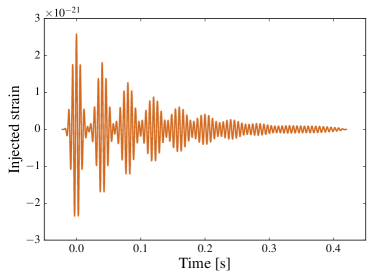
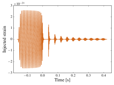
Figure 1: The simulated signals used to evaluate the method. Top panel: A train of sine-Gaussians. Bottom panel: the waveform from a toy model for a mass ratio $q=1000$ inspiral of a particle in a Schwarzschild spacetime, with Neumann reflective boundary conditions just outside the horizon.

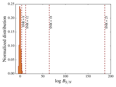
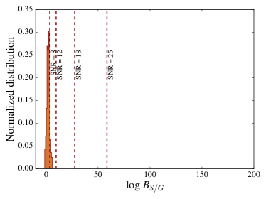
Figure 2: Background distributions for the (log) Bayes factors $B_{S/N}$ (top) and $B_{S/G}$ (bottom), containing 380 trials. The dashed lines show the values of these quantities for the injection of echoes from the inspiral toy model with SNRs of 8, 12, 18, and 25.

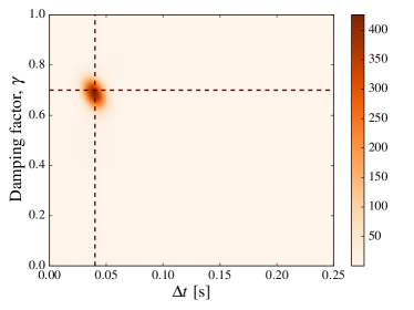
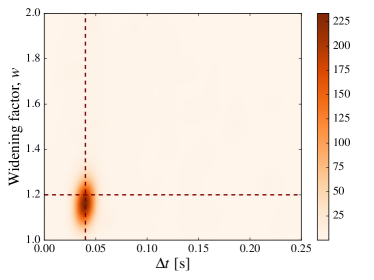
Figure 3: The distribution of samples for the case where the injected signal is a comb of sine-Gaussians. Top: Damping factor $\gamma$ against the time $\Delta t$ between echoes. Bottom: The widening factor $w$ against $\Delta t$. The colors indicate the number of samples per pixel, while the dashed lines show the true values of the parameters.

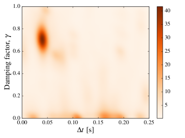
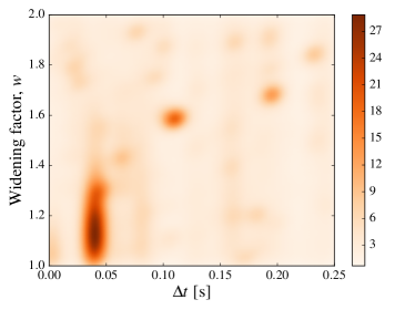
Figure 4: The distribution of samples for the case where the injected signal is the inspiral toy model. Again we show $\gamma$ versus $\Delta t$ (top) and $w$ versus $\Delta t$ (bottom).

Results. In order to test the algorithm we generate stationary, Gaussian noise for a network of two Advanced LIGO detectors at the predicted design sensitivity Abbott et al. (2013). In this we coherently inject (a) a single generalized wavelet as in Eq. (2), and (b) a train of echoes from a numerically solved toy model involving the inspiral of a particle in a Schwarzschild spacetime with Neumann reflective boundary conditions just outside the horizon, the mass ratio being $q=1000$ Price and Khanna (2017); Khanna and Price (2017). The signals are shown in Fig. 1. For case (a), one has $f_{0}=166.7$ Hz, $\tau=0.0095$ s, $\phi_{0}=0$, $\Delta t=0.04$ s, $\gamma=0.7$, and $w=1.2$. Both for cases (a) and (b), values for the amplitudes of the injected signals are chosen such that the combined (matched-filtering) signal-to-noise ratio (SNR) in all echoes is, respectively, 8, 12, 18, and 25. The higher values correspond to the SNR in the ringdown signal of a gravitational wave detection like GW150914 Abbott (2017) under the assumption that it would be seen in Advanced LIGO at final design sensitivity, whereas an SNR of 8 roughly equals the SNR that the ringdown actually had for GW150914 Abbott et al. (2016c).

For both types of simulated signals, 10 echoes are injected (in reality one would expect infinitely many), and the generalized wavelets used to characterize the simulated signals have 5 sine-Gaussians in them. Case (a) has a well-defined damping factor $\gamma$ and widening factor $w$, allowing us to establish that the method works as intended, by ascertaining that these parameters are recovered correctly. In case (b), $\gamma$ and $w$ may not have rigorous meaning, but the distributions on parameter space that are obtained should be indicative of the physics involved; moreover, the peaks of their distributions should correspond to what one estimates from a visual inspection of the signal. In the latter case, the stretch of data analyzed excludes the main signal, as one would also do in reality. In both cases the first echo is searched for in a window for $t_{0}$ that has a width of 0.5 s; for the other parameters the prior distributions are flat in $\Delta t\in[0,0.25]$ s, $\gamma\in[0,1]$, $w\in[1,2]$, and $\Delta\phi\in[0,2\pi]$.

In order to confidently detect echoes, the Bayes factors $B_{S/N}$ and $B_{S/G}$ must be compared with a background distribution for these quantities, computed on stretches of detector noise, e.g. at times immediately preceding the inspiral-merger-ringdown signal. These are shown in Fig. 2, together with the values obtained from the injection of echoes for the inspiral toy model. For all simulated signals considered here we find that, starting from SNR = 12, $\log B_{S/G}$ and $\log B_{S/N}$ are above their respective backgrounds; hence trains of echoes with this loudness would be detected with confidence. It is worth noting that very similar Bayes factors are obtained with the original BayesWave algorithm, which instead of the generalized wavelets of Eq. (2) uses the standard Morlet-Gabor wavelets consisting of single sine-Gaussians. Hence the use of generalized wavelets does not significantly improve detection. However, the generalized wavelets allow for the characterization of echoes, to which we now turn.

Fig. 3 shows the distribution of samples for case (a), for an SNR of 25 and injected echo-related parameters $\Delta t=0.04$ s, $\gamma=0.7$, and $w=1.2$. These are measured correctly, with peak values and standard deviations $\Delta t=0.040\pm 0.007$ s, $\gamma=0.69\pm 0.05$, and $w=1.16\pm 0.09$. In Fig. 4 we show the distribution of samples for case (b), again for an SNR of 25; visual inspection of the signal in Fig. 1 indicates similar values for $\Delta t$, $\gamma$, and $w$ as for case (a), and these are indeed the values where sample distributions have their main peaks. The peak values and standard deviations are $\Delta t=0.040\pm 0.007$ s, $\gamma=0.71\pm 0.11$, and $w=1.12\pm 0.12$. The distribution of $(w,\Delta t)$ samples also shows secondary peaks at $3\Delta t$ and $5\Delta t$. These correspond to secondary peaks with $\gamma\simeq 0$ in $(\gamma,\Delta t)$ space, which are cases where essentially only one echo was found. However, the secondary modes are considerably weaker than the main one. Finally, by looking at the injections with SNRs 18, 12, and 8, we checked that measurement uncertainties roughly increase with inverse SNR, as expected. We conclude that, given a sufficiently loud source, not only will we have the ability to detect the presence of echoes with high statstical confidence, we will also have a way to infer the properties of the exotic compact object.

Summary. We have constructed a method to search for, and characterize, gravitational wave echoes in a morphology-independent way. The algorithm decomposes the signal into generalized wavelets taking the form of “combs” of sine-Gaussians in order to capture the essence of echoes in the data. As in the original BayesWave, the evidences for three hypotheses are compared through a sampling over parameter space: signal, glitch, and Gaussian noise. We have shown that for a heuristic but physically motivated train of echoes, with plausible loudness given expected detector upgrades, the echoes signal can be confidently detected. We expect this to be the case for a wide variety of possible signal shapes corresponding to different types of compact objects, irrespective of an object’s detailed nature; in particular, no template waveforms are needed. Moreover, the distribution of samples over parameter space will reveal key characteristics of the echoes such as the time between successive bursts, as well as their widening and damping. This information can in turn be used to identify the nature of the potentially horizon-less merger remnant.

References

- Aasi et al. (2015) J. Aasi et al. (LIGO Scientific), Class.Quant.Grav. 32, 074001 (2015), eprint 1411.4547.
- Abbott (2017) B. P. Abbott (2017), pp. 291–311.
- Abbott et al. (2016a) B. P. Abbott et al. (Virgo, LIGO Scientific), Phys. Rev. Lett. 116, 241103 (2016a), eprint 1606.04855.
- Abbott et al. (2016b) B. P. Abbott et al. (Virgo, LIGO Scientific), Phys. Rev. X6, 041015 (2016b), eprint 1606.04856.
- Abbott et al. (2017a) B. P. Abbott et al. (VIRGO, LIGO Scientific), Phys. Rev. Lett. 118, 221101 (2017a), eprint 1706.01812.
- Abbott et al. (2017b) B. P. Abbott et al. (Virgo, LIGO Scientific), Astrophys. J. 851, L35 (2017b), eprint 1711.05578.
- Acernese et al. (2015) F. Acernese et al. (Virgo), Class. Quant. Grav. 32, 024001 (2015), eprint 1408.3978.
- Abbott et al. (2017c) B. P. Abbott et al. (Virgo, LIGO Scientific), Phys. Rev. Lett. 119, 141101 (2017c), eprint 1709.09660.
- Abbott et al. (2017d) B. Abbott et al. (Virgo, LIGO Scientific), Phys. Rev. Lett. 119, 161101 (2017d), eprint 1710.05832.
- Abbott et al. (2016c) B. P. Abbott et al. (Virgo, LIGO Scientific), Phys. Rev. Lett. 116, 221101 (2016c), eprint 1602.03841.
- Almheiri et al. (2013) A. Almheiri, D. Marolf, J. Polchinski, and J. Sully, JHEP 02, 062 (2013), eprint 1207.3123.
- Lunin and Mathur (2002) O. Lunin and S. D. Mathur, Nucl. Phys. B623, 342 (2002), eprint hep-th/0109154.
- Giudice et al. (2016) G. F. Giudice, M. McCullough, and A. Urbano, JCAP 1610, 001 (2016), eprint 1605.01209.
- Mazur and Mottola (2004) P. O. Mazur and E. Mottola, Proc. Nat. Acad. Sci. 101, 9545 (2004), eprint gr-qc/0407075.
- Liebling and Palenzuela (2012) S. L. Liebling and C. Palenzuela, Living Reviews in Relativity 15, 6 (2012), eprint 1202.5809.
- Cardoso et al. (2016a) V. Cardoso, E. Franzin, and P. Pani, Phys. Rev. Lett. 116, 171101 (2016a), [Erratum: Phys. Rev. Lett.117,no.8,089902(2016)], eprint 1602.07309.
- Cardoso et al. (2016b) V. Cardoso, S. Hopper, C. F. B. Macedo, C. Palenzuela, and P. Pani, Phys. Rev. D94, 084031 (2016b), eprint 1608.08637.
- Cardoso and Pani (2017) V. Cardoso and P. Pani, Nat. Astron. 1, 586 (2017), eprint 1709.01525.
- Abbott et al. (2016d) B. P. Abbott et al. (Virgo, LIGO Scientific), Phys. Rev. Lett. 116, 241102 (2016d), eprint 1602.03840.
- Abedi et al. (2017) J. Abedi, H. Dykaar, and N. Afshordi, Phys. Rev. D96, 082004 (2017), eprint 1612.00266.
- Westerweck et al. (2017) J. Westerweck, A. Nielsen, O. Fischer-Birnholtz, M. Cabero, C. Capano, T. Dent, B. Krishnan, G. Meadors, and A. H. Nitz (2017), eprint 1712.09966.
- Maselli et al. (2017) A. Maselli, S. H. Voelkel, and K. D. Kokkotas, Phys. Rev. D96, 064045 (2017), eprint 1708.02217.
- Mark et al. (2017) Z. Mark, A. Zimmerman, S. M. Du, and Y. Chen, Phys. Rev. D96, 084002 (2017), eprint 1706.06155.
- Cornish and Littenberg (2015) N. J. Cornish and T. B. Littenberg, Class. Quant. Grav. 32, 135012 (2015), eprint 1410.3835.
- Littenberg and Cornish (2015) T. B. Littenberg and N. J. Cornish, Phys.Rev. D91, 084034 (2015), eprint 1410.3852.
- Kanner et al. (2016) J. B. Kanner, T. B. Littenberg, N. Cornish, M. Millhouse, E. Xhakaj, F. Salemi, M. Drago, G. Vedovato, and S. Klimenko, Phys. Rev. D 93, 022002 (2016), eprint 1509.06423.
- Littenberg et al. (2016) T. B. Littenberg, J. B. Kanner, N. J. Cornish, and M. Millhouse, Phys. Rev. D94, 044050 (2016), eprint 1511.08752.
- Bécsy et al. (2017) B. Bécsy, P. Raffai, N. J. Cornish, R. Essick, J. Kanner, E. Katsavounidis, T. B. Littenberg, M. Millhouse, and S. Vitale, Astrophys. J. 839, 15 (2017), [Astrophys. J.839,15(2017)], eprint 1612.02003.
- Chatziioannou et al. (2017) K. Chatziioannou, J. A. Clark, A. Bauswein, M. Millhouse, T. B. Littenberg, and N. Cornish, Phys. Rev. D96, 124035 (2017), eprint 1711.00040.
- Millhouse et al. (2018) M. Millhouse, N. Cornish, and T. Littenberg (2018), in preparation.
- Abbott et al. (2013) B. P. Abbott et al. (VIRGO, LIGO Scientific) (2013), [Living Rev. Rel.19,1(2016)], eprint 1304.0670.
- Price and Khanna (2017) R. H. Price and G. Khanna, Class. Quant. Grav. 34, 225005 (2017), eprint 1702.04833.
- Khanna and Price (2017) G. Khanna and R. H. Price, Phys. Rev. D95, 081501 (2017), eprint 1609.00083.