Infinite dimensional adaptive MCMC for Gaussian processes

ABSTRACT. Latent Gaussian processes are widely applied in many fields like, statistics, inverse problems and machine learning. A popular method for inference is through the posterior distribution, which is typically carried out by Markov Chain Monte Carlo (MCMC) algorithms. Most Gaussian processes can be represented as a Gaussian measure in a infinite dimensional space. This is an issue for standard algorithms as they break down in an infinite dimensional setting, thus the need for appropriate infinite dimensional samplers for implementing probabilistic inference in such framework. In this paper, we introduce several adaptive versions of the preconditioned Crank–Nicolson Langevin (pCNL) algorithm, which can be viewed as an infinite dimensional version of the well known Metropolis-adjusted Langevin algorithm (MALA) algorithm for Gaussian processes. The basic premise for all our proposals lies in the idea of implementing change of measure formulation to adapt the algorithms to greatly improve their efficiency. A gradient–free version of pCNL is introduced, which is a hybrid of an adaptive independence sampler and an adaptive random walk sampler, and is shown to outperform the standard preconditioned Crank–Nicolson (pCN) scheme. Finally, we demonstrate the efficiency of our proposed algorithm for three different statistical models.

Key words: MCMC, Gaussian processes, preconditioned Crank–Nicolson, preconditioned Crank–Nicolson Langevin, infinite dimension, AMCMC, online estimation

1 Introduction

Sampling methods, particularly ones involving the Monte Carlo approach have been the subject of intense research activity for the past few decades. Markov Chain Monte Carlo (MCMC) method, a specific class of sampling approach, is used in sampling from intricate probability distributions, and is widely applicable in areas ranging from statistics, probability and many other areas.

In recent years, there has been considerable development of MCMC algorithms in the setting of infinite dimensional spaces (see [3, 19] ) where the classical, finite dimensional, MCMC algorithms fail to work. These algorithms can potentially be applied to various Bayesian inverse problems [18], and large class of problems in data assimilation (see Special Issue of Phys. D, Vol. 230, Issue 1–2 dedicated to data assimilation, and [1], in particular, for non-Gaussian data assimilation), and more recently in geostatistical models [9]. The distribution of interest in such applications is the posterior distribution, which has the cumulative information of the prior, and observations (data) emanating from the model under consideration. In practice, the posterior $\mu_{1}$ is specified as a density (the likelihood) with respect to a specific prior measure $\mu_{0}$:

$$\mu_{1}(du)=\exp(-\Phi(u,Y))\mu_{0}(du),$$ (1)

where $Y$ is the observations.

The state of the art infinite dimensional MCMC samplers are applicable whenever the target (posterior) distribution is assumed to be absolutely continuous with respect to a base Gaussian distribution, typically the prior distribution. Specifically, a class of MCMC algorithms (see [4]) use a clever Crank-Nicolson discretisation of an appropriate stochastic partial differential equation (SPDE), which forms the basis of underlying Markov chain, together with preconditioning which helps in tuning the efficiency of algorithm. This choice of SPDE leads to two major algorithms: the preconditioned Crank–Nicolson (pCN), which is the infinite dimensional analog of the Metropolis–Hastings random walk (MHRW), and the preconditioned Crank–Nicolson Langevin (pCNL), which is the infinite dimensional analog of Metropolis adjusted Langevin algorithm (MALA) (cf. [2]).

Since the emergence of [4], there have been many suggested modifications of the algorithms, in order to improve the mixing. As is the case with any MCMC sampler, the choice of dynamics for generation of new steps is crucial for mixing. Although the dynamics involved in pCN has the base Gaussian distribution as the invariant distribution, the Metropolis–Hastings acceptance/rejection step ensures that the algorithm has the correct target distribution. In [11] the author presents an approach which adapts the usual pCN to an operator version, and chooses the operator in an appropriate fashion so as to improve the efficacy of the proposed algorithm.

As can be seen from the vast literature concentrating on modifications of (Metropolis–Hastings adjusted) MCMC algorithms, many of the proposals centre around the theme of adaptation. Meaning, to learn the proposal distribution in either the first few steps of the algorithm, or during the entire run of the algorithm. The later version destroys the Markov property of the MCMC algorithm, however it is often the case that the limiting distribution of the algorithm is still the target density. We refer interested readers to [8] for one of the earliest implementation of adaptive schemes in MCMC, and [7] for a general summary and overview of results on adaptive MCMC schemes.

We shall focus on three specific adaptive schemes relevant to this paper. In [6] the authors consider infinite dimensional independence sampler MCMC algorithm, and propose a scheme to optimise the proposal parameters to achieve greater efficiency. The optimisation step involves searching for the Gaussian distribution which minimises its Kullback–Leibler divergence from the target distribution. Continuing on similar theme, the authors in [23] propose a hybrid MCMC adaptive scheme, which builds on [6] and addresses a specific drawback, that of dealing with the computational difficulty of evaluating square root of a given positive operator. The authors implement adaptive Metropolis scheme on an appropriately chosen finite dimensional subspace of the state space, and apply the usual pCN scheme on the complement. Recently in [21] the authors developed an elegant MCMC algorithm, the auxiliary sampler, which has the regular pCNL as a special case. In a series of applications, they showed great improvement in performance for the auxiliary gradient sampler compared to the standard infinite dimensional samplers.

The contribution of this paper, is three fold. We first note that one can reformulate (1) as

$$d\mu_{1}(u)=\exp(-\widetilde{\Phi}(u,Y))\,d\Psi(u),$$ (2)

where $\Psi$ is a Gaussian distribution which is equivalent to $\mu_{0}$, and $\widetilde{\Phi}(u,Y)=\Phi(u,Y)+\log\left(\frac{d\Psi}{d\mu_{0}}(u)\right)$. Using this reformulation, the pCN and pCNL algorithms are modified, while keeping the same target distribution. The extra degree of freedom, gained by choosing $\Psi$, allows us to create more efficient algorithms. Specifically, the algorithms proposed in [11, 23] can be related to (2) by choosing $\Psi$, in an appropriate fashion. Second, in the case when the gradient (of the log–likelihood) is not available, we propose an alternative for pCNL method. Instead of using the usual pCN, we use pCNL where the gradient is replaced by its expected value (under the posterior distribution). Incidentally, by the Fisher identity, the expected value equals the scaled posterior mean, i.e., ${\bf\mathsf{E}}[{\nabla}(-\Phi(u))]={\cal C}^{-1}{\bf\mathsf{E}}(u)$, where ${\cal C}^{-1}$ is the precision operator corresponding to $\mu_{0}$. We note here that the regular independence sampler is a special case of our proposed method (cf. [6]). Finally, we also discuss adapting our schemes to cases when the gradient and the Hessian of the log-likelihood are available.

We conclude the discussion about the proposals by comparing the efficiency of our algorithms against some known infinite dimensional sampler for three statistical problems. We show that the adaptive versions of the pCNL clearly outperform all the other algorithms.

Organisation of the paper: In Section 2, we first present some results related to Gaussian analysis which form the basis for all the discussion which follows. Subsequently, in Section 2.2 we discuss the existing MCMC based infinite dimensional samplers which form the foundation of our proposal schemes presented in later sections. We present some primary observations related to using the Kullback–Leibler divergence in Section 2.3, and integrate the findings with our proposals listed in Section 3. The analysis corresponding to listed proposals forms the crux of Section 4, where we furnish the related mathematical details. After presenting the practical aspect of implementing our proposals in Section 5, we finally demonstrate the experimental implication of our proposals in Section 6, and record our findings of comparative study with other known infinite dimensional samplers.

Finally, code for reproducing all the experiments are available at:
https://github.com/JonasWallin/Infinite_dimensional_adaptive_MCMC

2 Background

2.1 Gaussian measures in infinite dimensions

For the models studied in this paper, we shall restrict our attention only to Gaussian priors defined on appropriate Hilbert space. We shall now report relevant results from the literature concerning equivalence of Gaussian distributions in infinite dimensions.

As in the case of finite dimensions, a Gaussian measure in infinite dimensions is also characterised by its mean and covariance. We shall denote a Gaussian measure with mean $m$ and covariance ${\cal C}$ by ${\cal N}(m,{\cal C})$. For ${\cal N}(m,{\cal C})$ to be supported on a given Hilbert space, it is necessary that ${\cal C}$ be a trace class linear operator defined on the Hilbert space. For further analysis, we shall write $\|\cdot\|$ and $\langle\cdot,\cdot\rangle$ for the canonical norm and inner product on ${\cal H}$, We shall also define a weighted inner product $\langle\cdot,\cdot\rangle_{{\cal C}}=\langle{\cal C}^{-1/2}\cdot\,\,,{\cal C}^{-1/2}\cdot\rangle$, and the corresponding norm $\|\cdot\|_{{\cal C}}=\|{\cal C}^{-1/2}\cdot\|$. With these definitions, one can define the Cameron–Martin space corresponding to the covariance operator ${\cal C}$ as ${\cal H}_{{\cal C}}=\{x\in{\cal H}:\,\|{\cal C}^{-1/2}x\|<\infty\}$.

It is well known that two Gaussian measures defined on the same finite dimensional space are always absolutely continuous to one another. However, the statement is not true for Gaussian measures on infinite dimensional spaces. We shall present the following well known result concerning equivalence of Gaussian measures on Hilbert spaces (cf. [10, Theorem 3.4]).

Lemma 2.1 (Feldman–Hajek).

Two Gaussian measures ${\cal N}(m_{1},{\cal C}_{1})$ and ${\cal N}(m_{2},{\cal C}_{2})$ on the Hilbert space ${\cal H}$ are either equivalent, or orthogonal. They are equivalent if and only if,

• $\left(m_{1}-m_{2}\right)\in{\cal H}_{{\cal C}_{1}}$, and

• the linear operator $\left({\cal C}_{1}^{-1/2}{\cal C}_{2}{\cal C}_{1}^{-1/2}-{\cal I}\right)$ is Hilbert–Schmidt.

Remark 2.2.

The conditions stated above to check for equivalence of two Gaussian measures can further be simplified for specific cases. For instance, consider ${\cal N}(0,\Lambda_{1})$ and ${\cal N}(0,\Lambda_{2})$, where $\Lambda_{1}$ and $\Lambda_{2}$ are diagonal, with $\{\lambda_{i,1}\}_{i\geq 1}$ and $\{\lambda_{i,2}\}_{i\geq 1}$ as the diagonal entries, respectively. Then the condition for equivalence of ${\cal N}(0,\Lambda_{1})$ and ${\cal N}(0,\Lambda_{2})$ simplifies to checking $\sum_{i\geq 1}\left(\frac{\lambda_{i,1}}{\lambda_{i,2}}-1\right)^{2}<\infty$.

2.2 Overview of MCMC methods in infinite dimensions

As stated earlier, our interested lies in MCMC methods for sampling from measure $\mu_{1}$ on infinite dimensional Hilbert space, say ${\cal H}$. Characterising measures in infinite dimensions is often an intricate problem, and it is often desirable to define the concerned measure in infinite dimensions via another well defined measure on the same space, called the base measure. Mostly, the base measure is taken to be a Gaussian distribution with known mean and covariance. We, therefore, set $\mu_{0}$ to be a known, mean zero Gaussian measure with covariance ${\cal C}$ as the base measure, such that target measure $\mu_{1}$ satisfies

$$\frac{d\mu_{1}}{d\mu_{0}}(u)=\exp\left(-\Phi(u)\right).$$ (3)

Remark 2.3.

(Notational remark) In what follows, we shall set $\{\varphi_{k}\}_{k\geq 1}$ to be the canonical basis of the Hilbert space ${\cal H}$, and $\{(\sigma_{k},e_{k})\}_{k\geq 1}$ to be the ordered set of eigen pairs of the covariance operator ${\cal C}$, such that $\sigma_{1}\geq\sigma_{2}\geq\sigma_{3}\geq\ldots$. Thus enabling us to write ${\cal C}=\sum_{k\geq 1}\sigma_{k}\langle\cdot,e_{k}\rangle e_{k}$.

Further borrowing notation and inspiration from [4], we reiterate that all the algorithms and methods discussed in this paper are derived from discretisation of an appropriate SPDE. Setting $B$ as the standard Brownian motion, ${\cal K}$ and ${\cal L}$ for linear operators chosen appropriately in relation to the prior (base) measure $\mu_{0}$, the SPDE is given by

$$\frac{\partial u}{\partial s}=-{\cal K}\left({\cal L}u+\gamma{\nabla}\Phi(u)\right)+\sqrt{2{\cal K}}\frac{dB}{ds},$$ (4)

where, ${\nabla}\Phi:X\to X$ is the Nemitski operator (cf. [3]), and $\gamma$ is a tuning parameter which is indicative of the invariant measure of the SPDE. In particular, with ${\cal L}={\cal C}^{-1}$, and any positive linear operator ${\cal K}$, the above dynamics has

• $\mu_{0}$ as the invariant measure whenever $\gamma=0$;

• $\mu_{1}$ as the invariant measure whenever $\gamma=1$.

In [4], the authors discussed and analysed MCMC methods based on discretisation of (4). Here we give a short review of the methods used for sampling from infinite dimensional Gaussian processes, which will form the foundation for our methods.

A Metropolis–Hastings sampler involves two steps: a proposal step, followed by an adjustment. The first step to generate a proposal, uses a discrete time approximation of an appropriate dynamics, say (4) in the infinite dimensional setup. Subsequently, the proposal is then accepted, or rejected, based on evaluation of certain likelihood to rule out any inherent bias in the proposal. For instance, one can choose to ignore the drift terms in (4), and thus generate samples in the MCMC step which have absolutely no information about the target measure. The adjustment step then ensures that the process eventually mimics the target distribution.

It is not difficult to notice that one can generate a $1$-parameter family of discretisations of (4) by writing (cf.[3, 4])

$$v=u-\delta\theta{\cal K}{\cal L}\,u-\delta(1-\theta){\cal K}{\cal L}\,v-\gamma\delta{\cal K}{\nabla}\Phi(u)+\sqrt{2{\cal K}\,\delta}\,\xi,$$ (5)

where $\theta\in[0,1]$, $\xi$ is a (spatial) white noise. The above can be rewritten as

$$v=\left({\cal I}+\delta(1-\theta){\cal K}{\cal L}\right)^{-1}\,\left[\left({\cal I}-\delta\theta{\cal K}{\cal L}\right)\,u-\gamma\delta{\cal K}{\nabla}\Phi(u)+\sqrt{2{\cal K}\,\delta}\,\xi\right].$$ (6)

In this paper, we shall restrict our attention to a specific case, that of $\theta=\frac{1}{2}$, and discuss some known, and introduce some new methods to generate proposals, given the initial state.

After specifying the proposal step, we invoke the Metropolis–Hastings step, for which we write $q(u,dv)$ for the conditional distribution of $v|u$. Then writing $\nu$ for the joint distribution of $(u,v)$ given by $\nu(du,dv)=q(u,dv)\,\mu(du)$, and $\nu^{\perp}$ for the measure obtained by reversing the roles of $u$ and $v$ when defining $\nu(du,dv)$, the proposal $v$ is accepted with probability

$$\alpha(v,u)=\min\left(1,\frac{d\nu^{\perp}}{d\nu}(u,v)\right),$$ (7)

where $\frac{d\nu^{\perp}}{d\nu}(u,v)$ denotes the Radon–Nikodym derivative of $\nu^{\perp}$ with respect to $\nu$. To this end, we note that the Radon–Nikodym derivative in (7) is obtained via a third measure, say $\nu_{\star}$ on $X\times X$, as

$$\frac{d\nu^{\perp}}{d\nu}(u,v)=\frac{d\nu^{\perp}}{d\nu_{\star}}(u,v)\left(\frac{d\nu}{d\nu_{\star}}(u,v)\right)^{-1}.$$ (8)

Throughout the rest of this paper, we shall assume that the potential $\Phi$ introduced in (3) satisfies the following regularity conditions.

• There exist $p,K>0$ such that

  $$0\leq\Phi(u)\leq K\left(1+\|u\|^{p}\right)\,\,\,\,\,\forall u\in X;$$

• $\forall r>0$, there exists $K(r)>0$ such that

  $$\sup_{\|u\|,\|v\|<r}\frac{|\Phi(u)-\Phi(v)|}{\|u-v\|}\leq K(r),\,\,\,\,\,\text{and }\,\,\,\,\,\,\,0<K(r)<\left(1+r^{q}\right)$$

  for some $q>0$.

• For the eigen basis $\{e_{k}\}$ of ${\cal C}$, and a random variable $\zeta\sim\mu_{1}$, let $\zeta_{k}=\langle\zeta,e_{k}\rangle$, then we assume that

  $$\sum_{k\geq 1}\left(\frac{\text{var}(\zeta_{k})}{\sigma_{k}}-1\right)^{2}<\infty,$$

These assumptions are necessary for various measures and densities to be well defined later in our analysis. Assumptions (A1)–(A2) are natural, and can be found to be rooted in the context of Bayesian inverse problems (see [18, Assumption 2.6]), and the last assumption (A3) is needed to incorporate the Kullback–Leibler optimisation within the proposed MCMC algorithms.

2.2.1 Preconditioned Crank–Nicolson proposal (pCN)

Using (6) as a template for generating proposals, it was proposed in [4] to set ${\cal L}={\cal C}^{-1}={\cal K}^{-1}$, and $\gamma=0$, with $\theta=\frac{1}{2}$. The MCMC proposal is then stated as

$$v=(1-\beta^{2})^{1/2}u+\beta\mathcal{C}^{1/2}\xi,$$ (9)

where $\xi\sim N(0,\mathcal{I})$, and $\beta^{2}=8\delta/(2+\delta)^{2}$. Let us denote $q_{pCN}(u,dv)$ for the Gaussian measure ${\cal N}\left((1-\beta^{2})^{1/2}u,\,\,\beta^{2}{\cal C}\right)$, and set $\nu_{\star}$ as the Gaussian measure corresponding to $q_{pCN}(u,dv)\mu_{0}(du)$. Then, the Radon–Nikodym derivative of $\nu$ with respect to $\nu_{\star}$ is given by

$$\frac{d\nu}{d\nu_{\star}}(u,v)=\exp\left(-\Phi(u)\right).$$ (10)

In order to also incorporate the effect of $v$, it is customary to write

$$\frac{d\nu}{d\nu_{\star}}(u,v)=\exp\left(-\rho(u,v)\right),$$ (11)

implying that $\rho(u,v)=\Phi(u)$ for the pCN scheme.

Reversing the roles of $u$ and $v$, we set $\nu^{\perp}_{\star}(du,dv)=q_{pCN}(v,du)\mu_{0}(dv)$. However, notice that $\nu^{\perp}_{\star}=\nu_{\star}$. Therefore,

$$\frac{d\nu^{\perp}}{d\nu^{\perp}_{\star}}(u,v)=\frac{d\nu^{\perp}}{d\nu_{\star}}(u,v)=\exp\left(-\Phi(v)\right),$$ (12)

implying

$$\frac{d\nu^{\perp}}{d\nu}(u,v)=\exp\left({\cal J}_{pCN}(u,v)\right).$$ (13)

where ${\cal J}_{pCN}(u,v)=\Phi(u)-\Phi(v)$. Thus, in this method, the acceptance probability given by

$$\alpha_{pCN}(v,u)=\min\left(1,\exp\left({\cal J}_{pCN}(u,v)\right)\right)$$ (14)

depends solely on the potential $\Phi$.

2.2.2 Preconditioned Crank–Nicolson Langevian propsal (pCNL)

As noted earlier, by setting $\gamma=0$, the samplers thus generated use dynamics which keep the noise measure invariant. However, heuristically it is desirable to use the dynamics which keeps the target measure invariant, which then points at setting a nonzero $\gamma$ in (6), leading to what are known as the Crank–Nicolson Langevin (CNL), and preconditioned Crank–Nicolson Langevin (pCNL) proposals, corresponding to ${\cal K}={\cal I}$ and ${\cal K}={\cal C}$, respectively.

We shall focus on pCNL proposals, which can be expressed as

$$v=(1-\beta^{2})^{1/2}u-(1-(1-\beta^{2})^{1/2}){\cal C}{\nabla}\Phi(u)+\beta\mathcal{C}^{1/2}\xi,$$ (15)

where $\xi\sim N(0,\mathcal{I})$, and $\beta^{2}=\frac{8\delta}{(2+\delta)^{2}}\in[0,1]$. Again setting $\nu_{\star}(du,dv)=q_{pCN}(u,dv)\mu_{0}(du)$, and using the notation set forth in (11), we obtain

$$\rho(u,v)=\Phi(u)+\frac{\delta}{4}\|{\cal C}^{1/2}{\nabla}\Phi(u)\|^{2}+\frac{1}{2}\langle v-u,{\nabla}\Phi(u)\rangle+\frac{\delta}{4}\langle v+u,{\nabla}\Phi(u)\rangle,$$ (16)

where, for the equivalence of $\nu$ and $\nu_{\star}$, we need $\|{\cal C}^{1/2}{\nabla}\Phi(u)\|<\infty$, $\mu$ almost surely, which is clearly satisfied under the assumptions (A1) and (A2).

Again, by the symmetry of $\nu_{\star}$, we have $\nu^{\perp}_{\star}=\nu_{\star}$, thus

$$\frac{d\nu^{\perp}}{d\nu^{\perp}_{\star}}(u,v)=\frac{d\nu^{\perp}}{d\nu_{\star}}(u,v)$$ (17)

Thus, the acceptance probability is given by

$$\alpha_{pCNL}(v,u)=\min\left(1,\exp\left({\cal J}_{pCNL}(u,v)\right)\right),$$

where

$${\cal J}_{pCNL}(u,v) = \Phi(u)-\Phi(v)+\frac{\delta}{4}\left(\|{\cal C}^{1/2}{\nabla}\Phi(u)\|^{2}-\|{\cal C}^{1/2}{\nabla}\Phi(v)\|^{2}\right)$$

$$+\frac{1}{2}\Big{\langle}v-u,{\nabla}\Phi(u)+{\nabla}\Phi(v)\Big{\rangle}+\frac{\delta}{4}\Big{\langle}v+u,{\nabla}\Phi(u)-{\nabla}\Phi(v)\Big{\rangle}.$$

2.3 Kullback–Leibler divergence

As stated earlier, our goal is to amalgamate the standard infinite dimensional sampler discussed above with adaptive schemes. The idea of implementing adaptive schemes centres around the heuristic that adaptive schemes work very well when incorporating the knowledge of the target measure.

In the pCN approach discussed in Section 2.2.1, setting $\beta=1$ in (9) defines what is commonly known as the independence sampler. In the infinite dimensional setup, every new proposal in independence sampler is chosen to be Gaussian. However, since every Gaussian measure is characterised by its mean and covariance, one could choose these parameters optimally so as to achieve better efficiency. A natural measure for optimality is the Kullback–Leibler (KL) divergence, which is also referred to as the relative entropy in information theoretic parlance. This precise idea of optimally choosing parameters of the Gaussian measure involved in generating proposals has been studied in [13, 14]. As can be seen in the stated literature, the problem is difficult, theoretically and computationally. Playing on the asymmetry of KL divergence, the authors in [6] propose a slight modification of [14] by swapping the arguments involved in the KL divergence. Although, in [14] the authors present an argument in favour of their choice of KL divergence, however, due to the computational complexity involved in making such choice, we shall choose to optimise the KL divergence as in [6].

We note here that the choice of parameterisation of Gaussian measure is critical to the analysis that follows. Recall that we have chosen $\{\varphi_{k}\}_{k\geq 1}$ to be the canonical orthonormal basis of ${\cal H}$, and $\{(\sigma_{k},e_{k})\}_{k\geq 1}$ as the ordered set of eigen pairs of the covariance ${\cal C}$. Further for the ease of notation, we shall define $\Sigma$ to be the self adjoint linear operator defined by

$$\langle\varphi_{i},\Sigma\varphi_{j}\rangle=\sigma_{i}\delta^{i}_{j},$$ (18)

where $\delta^{i}_{j}$ is the Kronecker delta, and finally, we set ${\cal P}$ as the unitary operator defined by ${\cal P}^{T}\varphi_{i}=e_{i}$, for all $i\geq 1$. Therefore, with these notations, we can write

$${\cal C}={\cal P}\Sigma{\cal P}^{T}.$$ (19)

As suggested earlier, we shall choose to optimise the KL divergence over the set of Gaussian measures with mean $m$, an arbitrary element in ${\cal H}_{{\cal C}}$, and covariance given by ${\cal S}\Lambda{\cal S}^{T}$, where ${\cal S}={\cal P}\Sigma^{1/2}$, and $\Lambda$ is a self adjoint positive operator which is diagonalisable in the canonical basis $\{\varphi_{k}\}_{k\geq 1}$. Note that in this notation, we could write ${\cal C}={\cal S}{\cal S}^{T}$, and the covariance ${\cal S}\Lambda{\cal S}^{T}$ can be seen to be simply a multiplicative perturbation of the eigen values of ${\cal C}$. A multiplicative perturbation appears to be a natural choice for the purposes of this paper, however, there are other ways of introducing covariance operators in relation to the prior covariance. The authors in [6], for instance, consider instead an additive perturbation of the precision operator ${\cal C}^{-1}$, such that the perturbation is diagonalisable in the same basis as that of ${\cal C}$. With regards to computational complexity, and efficiency of algorithms, the additive and multiplicative perturbative schemes are equivalent in the case when the perturbation and ${\cal C}$ are simultaneously diagonalisable.

Specifically, writing $\Psi$ for Gaussian measure with mean $m$ and covariance ${\cal S}\Lambda{\cal S}^{T}$, the Kullback–Leibler divergence, denoted by $\delta$ between the target measure $\mu_{1}$ and $\Psi$ can be expressed as

$$\delta(\mu_{1}\|\Psi) = \int\log\left(\frac{d\mu_{1}}{d\Psi}\right)\,d\mu_{1}=\int\left(\log\left(\frac{d\mu_{1}}{d\mu_{0}}\right)-\log\left(\frac{d\Psi}{d\mu_{0}}\right)\right)\,d\mu_{1}$$

$$= \int\left(-\Phi(x)-\log\left(\frac{d\Psi}{d\mu_{0}}\right)\right)\,d\mu_{1},$$

where $\frac{d\Psi}{d\mu_{0}}$ is given by the Feldman–Hajek Theorem. Using the notation of [10, Chapter 2, Theorem 3.3] we can write $\frac{d\Psi}{d\mu_{0}}$ as

$$\frac{d\Psi}{d\mu_{0}}(x) = \exp\left[\langle({\cal K}^{-1}x,m\rangle-\frac{1}{2}\langle{\cal K}^{-1}m,m\rangle\right]\times\left(\prod_{k\geq 1}\frac{1}{\sqrt{d_{k+1}}}\right)\exp\left[\frac{1}{2}\langle({\cal C}^{-1}-{\cal K}^{-1})x,x\rangle\right]$$

where $\{d_{k}\}$ are the eigen values of $\Lambda$, and we have inherently assumed that the Gaussian measures with covariances ${\cal S}\Lambda{\cal S}^{T}$ and ${\cal S}{\cal S}^{T}$ are equivalent. Therefore, the KL divergence can be rewritten as

$$\delta(\mu_{1}\|\Psi) = -\int\Phi(x)\,d\mu_{1}(x)+\frac{1}{2}\sum_{k\geq 1}\log d_{k+1}$$

$$-\int\sum_{i\geq 1}\left(\frac{\langle x,e_{i}\rangle^{2}}{2}\left(\frac{1}{\sigma_{i}}-\frac{1}{d_{i}\sigma_{i}}\right)-\frac{\langle m,e_{i}\rangle\langle x,e_{i}\rangle}{d_{i}\sigma_{i}}-\frac{1}{2}\frac{\langle m,e_{i}\rangle^{2}}{d_{i}\sigma_{i}}\right)\,d\mu_{1}(x)$$

Minimising the above over the parameters $m$ and $\{d_{k}\}$, for $k\geq 1$, we shall obtain the minimisers,

$$m_{\star}={\bf\mathsf{E}}[u],$$ (20)

and

$$d_{\star,k}=\frac{1}{\sigma_{k}}\int\langle x-m_{\star},e_{k}\rangle^{2}\,d\mu_{1},$$ (21)

Therefore, as in the finite dimensional case, the best Gaussian approximation to the target measure is one which has the same mean and variance as that of target measure.

As noted earlier in Lemma 2.1, for $\Psi$ to be equivalent to $\mu_{0}$, it is necessary (and sufficient) that $m$ belongs to ${\cal H}_{{\cal C}}$, and that $\{d_{k}\}$ satisfy $\sum_{k\geq 1}\left(d_{k}-1\right)^{2}<\infty$. Therefore, in order for us to use the optimal parameters found in (20) and (21), we must ensure that $\{m_{\star,k}\}$ and $\{d_{\star,k}\}$ satisfy the same set of assumptions. Notice, however, that ${\bf\mathsf{E}}\left[{\nabla}\Phi(u)\right]=-{\cal C}^{-1}\,m_{\star}$, which can be obtained using Fisher’s identity in infinite dimensions. Now recall that $\|{\nabla}\Phi(u)\|^{2}<\infty$ for all $u\in{\cal H}$, therefore, ${\cal C}^{-1}m_{\star}\in{\cal H}$, implying that $m_{\star}\in{\cal H}_{{\cal C}}$. With regards the regularity condition on $\{d_{\star,k}\}$, assumption (A3) ensures that it is satisfied.

Remark 2.4.

We note here that the assumption (A3) concerning the directional variances of the target measure is well founded. Specifically, if the target measure were Gaussian, then the most basic assumption regarding equivalence of the target and the base measure implies that the above assumptions concerning the directional variance of the target measure are unconditionally satisfied.

In the following sections, we shall incorporate the above findings with the proposals discussed in Sections 2.2.1 and 2.2.2.

3 Our proposals and results

In this section, we shall introduce our main adaptive proposals, which originate from changing the underlying measure as mentioned in the introduction. A modulated version of the usual pCNL is obtained by replacing ${\cal K}={\cal C}$ with ${\cal K}={\cal S}\Lambda_{\star}{\cal S}^{T}$, where $\Lambda_{\star}$ is a self adjoint operator with its eigen pairs given by $\{(d_{\star,k},\varphi_{k})\}_{k\geq 1}$, with $d_{\star,k}$ as defined in the previous section.

As can be observed from our discussion in Section 2.2, not only that the choice of ${\cal L}$ dictates the base measure $\mu_{0}$, but choosing ${\cal L}={\cal K}^{-1}$ simplifies the computations considerably. The change of measure step corresponds to choosing ${\cal L}={\cal K}^{-1}=({\cal S}^{T})^{-1}\Lambda^{-1}_{\star}{\cal S}^{-1}$. By choosing ${\cal L}$ to be so, the base measure changes to Gaussian measure with covariance ${\cal S}\Lambda_{\star}{\cal S}^{T}$, which in turn changes the “target measure” related to the dynamics of the SPDE, since the target measure is known via the base measure. Thus, in order to keep the target measure firmly in our sight, we need to keep the base measure unchanged, which thus warrants appropriate modification of the potential, as hinted at in the introduction. Here, we present the resulting algorithms, and we shall defer the related analysis to later subsections.

For each algorithm stated below, the acceptance probability of a proposal $v$ given $u$ is denoted by $\alpha(v,u)=\min(1,\exp({\cal J}(v,u)))$, where we suffix $\alpha$ and ${\cal J}$ with appropriate acronyms to differentiate various algorithms. We now state the algorithms with a note that we set $\xi\sim N(0,\mathcal{I})$ in all the following algorithms.

Next, as stated in the introduction, when ${\nabla}\Phi(u)$ is not available, we replace it with ${\bf\mathsf{E}}[{\nabla}\Phi(u)]=-{\cal C}^{-1}{\bf\mathsf{E}}[u]$. This results in MCMC proposals which appear very similar to the regular pCN, and thus we denote our proposals as such with appropriate suffixes.

The last proposal deals with changing the base measure using the Hessian

We also incorporated another elementary adaptation technique, which is to modify the preconditioner ${\cal K}$, without changing the measure. This rather straightforward adaptation of algorithms presented in [4] has been implemented and the experimental results stated in Section 6. The corresponding analysis is documented in Appendix A.

4 Changing the base measure

As has been pointed earlier in the introduction, when using (6) for generating new proposals, we could set ${\cal L}$ to be different from ${\cal C}^{-1}$, as against the usual pCN. However, since ${\cal L}$ is closely related to the base Gaussian measure, changing ${\cal L}$ implies that we shall need to adjust the potential $\Phi$ appropriately so as to retain the same target measure.

Let us begin with setting ${\cal L}={\cal K}^{-1}=({\cal S}^{T})^{-1}\Lambda_{\star}^{-1}{\cal S}^{-1}$, allowing us to retain the same coefficients for $u$ as in pCN or pCNL in the discretization step. As indicated earlier, since ${\cal L}$ relates to the base Gaussian measure, choosing such ${\cal L}$ as above, changes the target measure to $d\mu^{*}_{1}=\exp\left(-\Phi(u)\right)\,d\mu^{*}_{0},$ where $\mu^{*}_{0}$ is ${\cal N}(0,{\cal S}\Lambda_{\star}{\cal S}^{T})$.

Nevertheless, the desired target measure $\mu_{1}$ can also be expressed in terms of $\mu^{*}_{0}$, but with a modified potential. In particular,

$$\frac{d\mu_{1}}{d\mu^{*}_{0}}(u)=\frac{d\mu_{1}}{d\mu_{0}}(u)\,\frac{d\mu_{0}}{d\mu^{*}_{0}}(u)=\exp\left(-\Phi(u)\right)\frac{d\mu_{0}}{d\mu^{*}_{0}}(u).$$

It is not difficult to notice

$$\frac{d\mu_{0}}{d\mu^{*}_{0}}(u)=\text{constt.}\,\exp\left(-\frac{1}{2}\left\langle({\cal S}^{T})^{-1}\left({\cal I}-\Lambda_{\star}^{-1}\right){\cal S}^{-1}u,u\right\rangle\right)$$

where the summability condition of $\{d_{\star,k}\}_{k\geq 1}$ discussed earlier ensures that $\mu_{0}$ is equivalent to $\mu^{*}_{0}$. Subsequently, the potential with respect to the new base measure is given by

$$\widetilde{\Phi}(u)=\Phi(u)+\frac{1}{2}\left\langle({\cal S}^{T})^{-1}\left({\cal I}-\Lambda_{\star}^{-1}\right){\cal S}^{-1}u,u\right\rangle.$$

Therefore, the $\text{pCNL}_{\text{AM}}$ proposal then can be written as

$$v=(1-c_{\beta})\,u+c_{\beta}m(u)+\beta\,{\cal S}z,$$ (22)

where $c_{\beta}=1-(1-\beta^{2})^{1/2}$ and $m(u)=u-{\cal S}\Lambda_{\star}({\cal S}^{T}{\nabla}\Phi(u)+{\cal S}^{-1}u)$ and $z\sim{\cal N}(0,\Lambda_{\star})$. The corresponding Metropolis–Hasting ratio is

$${\cal J}_{\text{pCNL}_{\text{AM}}}(v,u) = \Phi(u)-\Phi(v)+\frac{1}{2}\langle{\cal S}^{-1}v,(\Lambda^{-1}_{\star}-{\cal I}){\cal S}^{-1}v\rangle-\frac{1}{2}\langle{\cal S}^{-1}u,(\Lambda^{-1}_{\star}-{\cal I}){\cal S}^{-1}u\rangle$$

$$-\frac{c_{\beta}}{\beta^{2}}\langle m(u),v-(1-c_{\beta})u-\frac{1}{2}c_{\beta}m(u)\rangle_{{\cal K}}$$

$$+\frac{c_{\beta}}{\beta^{2}}\langle m(v),u-(1-c_{\beta})v-\frac{1}{2}c_{\beta}m(v)\rangle_{{\cal K}}.$$

Notice that in order to implement the above scheme, we needed to ensure that $\delta\{-u+\Lambda_{\star}({\cal C}{\nabla}\Phi(u)+u)\}$ be in the Cameron–Martin space of ${\cal S}\Lambda_{\star}{\cal S}^{T}$ almost surely with respect to the target measure $\mu_{1}$. However, this condition can be shown to be satisfied without invoking anymore assumptions. First, recall that $\|{\nabla}\Phi(u)\|^{2}<\infty$ almost surely $\mu_{1}$, then observe that ${\bf\mathsf{E}}\left({\nabla}\Phi(u)\right)=-{\cal C}^{-1}{\bf\mathsf{E}}(u)$, which assures that the aforementioned condition is indeed satisfied.

In the example below we illustrate that proposal distributions for pCN with changed measure contains some, trivial, posterior distribution. We will in the next section show how one can extend the pCN algorithm so it contains non trivial posterior distributions of non trivial examples.

Remark 4.1.

If in a finite dimensional case we have a prior for $u$ of the form $\mathcal{N}(0,{\cal P}^{T}\Sigma{\cal P})$, and a likelihood of the form $\exp(-\frac{1}{2}\left(y-u\right)^{T}\left(y-u\right))$. Then in the special case that $y=0$, the posterior distribution is contained in the pCN proposal by setting $\Lambda^{-1}_{\star}=\Sigma+\mathcal{I}$.

We next proceed towards further computational simplicity of implementing the above scheme. Often in many applications, one can only evaluate the potential $\widetilde{\Phi}$, however, the algorithm for proposal generation requires the evaluation of the gradient of the potential, leading us to investigate various methods to replace, or approximate ${\nabla}\widetilde{\Phi}$. We shall marry the above observations with the findings discussed in the beginning of Section 3 to appropriately modulate $\widetilde{\Phi}$.

4.1 Expectation approximation of gradient

The first method we propose is an adaptive version of the sampler discussed above where we replace the gradient part with its zeroth order approximation, i.e., its expectation with respect to the target measure. This is the method we denoted $\text{pCN}_{\text{AM}}$ above. Recall that the optimal mean of the Gaussian step/proposal evaluated earlier is precisely the mean of the target measure. One can see, from simple calculations, that

$${\bf\mathsf{E}}\left({\nabla}\widetilde{\Phi}(u)\right)={\bf\mathsf{E}}\left({\nabla}\Phi(u)+({\cal S}^{T})^{-1}\left({\cal I}-\Lambda_{\star}^{-1}\right){\cal S}^{-1}u\right)$$

where ${\bf\mathsf{E}}$ denotes expectation with respect to the target measure. Since ${\nabla}\Phi$, being a Nemitski operator, is a natural extension of finite dimensional gradient, we have that ${\bf\mathsf{E}}\left({\nabla}\Phi(u)\right)=-{\cal C}^{-1}m$, and thus

$${\bf\mathsf{E}}\left({\nabla}\widetilde{\Phi}(u)\right)=-\,({\cal S}^{T})^{-1}\Lambda_{\star}^{-1}{\cal S}^{-1}m.$$

Thus we now replace $m(u)$ with $m$ resulting in a Crank Nicolson like proposal:

$$v=(1-\beta^{2})^{1/2}u+(1-(1-\beta^{2})^{1/2})m+\beta{\cal S}z,$$

where $z\sim\mathcal{N}(0,\Lambda_{\star})$ Since $m$ is invariant under $u$ the Metropolis Hasting ratio simplifies to

$${\cal J}_{\text{pCN}_{\text{AM}}}(v,u) = \Phi(u)-\Phi(v)+\frac{1}{2}\langle S^{-1}v,(\Lambda^{-1}_{\star}-{\cal I})S^{-1}v\rangle-\frac{1}{2}\langle S^{-1}u,(\Lambda^{-1}_{\star}-{\cal I})S^{-1}u\rangle$$

$$-\langle(v-u),m\rangle_{{\cal K}}.$$

Remark 4.2.

If in a finite dimensional case we have a prior for $u$ on the form $\mathcal{N}(0,{\cal P}^{T}\Sigma{\cal P})$ and a likelihood of the form $\exp(-\frac{1}{2}\left(y-u\right)^{T}\left(y-u\right))$. Then the posterior distribution is contained in the $\text{pCN}_{\text{AM}}$ proposal by setting $\Lambda^{-1}_{\star}=\Sigma+\mathcal{I}$ and setting $m_{\star}=S^{T}\Lambda_{\star}S\frac{y}{\sigma^{2}}$.

4.1.1 Changing the base measure using Hessian

In case the Hessian, $H(u)=-\nabla\nabla\Phi(u)$, of the potential, $\Phi(u)$, is available (and computationally feasible) one can use this for a one can generate an adaptive base measure with covariance operator $\left({\cal C}^{-1}+H(u)\right)^{-1}$. This results in second order $\text{pCNL}_{\text{HM}}$ algorithm. We omit the tedious details, and just state the proposal and Metropolis–Hastings proposal given by

$$v=(1-c_{\beta})u+c_{\beta}m(u)+\beta(\mathcal{C}^{-1}+H(u))^{-1/2}\xi,$$ (23)

where $\xi\sim N(0,\mathcal{I})$ and

$$m(u)=(\mathcal{C}^{-1}+H(u))^{-1}(\nabla\Phi(u)-\mathcal{C}^{-1}u).$$

The corresponding Metropolis–Hasting ratio is given by

$${\cal J}_{\text{pCNL}_{\text{HM}}}(v,u) =\Phi(v)-\Phi(u)$$ (24)

$$+\frac{0.5}{\beta^{2}}\langle v-c_{\beta}u,v-c_{\beta}u\rangle_{H(u)}-\frac{0.5}{\beta^{2}}\langle u-c_{\beta}v,u-c_{\beta}v\rangle_{H(u)}$$

$$+\frac{c_{\beta}}{\beta^{2}}\langle m(v),u-(1-\beta^{2})^{1/2}v-0.5c_{\beta}m(v)\rangle_{C^{-1}+H(v)}$$

$$-\frac{c_{\beta}}{\beta^{2}}\langle m(u),v-(1-\beta^{2})^{1/2}u-0.5c_{\beta}m(u)\rangle_{C^{-1}+H(u)}.$$

We will explore this algorithm in one experiment below, where the Hessian can be computed efficiently. We omit the preconditioned version, $\text{pCNL}_{\text{HP}}$, due the fact that it includes computing a series matrix inverses that are computationally infeasible in our experiments..

5 Infinite dimensional estimation

As discussed in Section 2.3, there are two sets of parameters to be estimated for implementing our proposals. We used the mean $m_{\star}$ of the target distribution as a replacement for the gradient term in pCNL for our proposals in Section 4.1. In this section, we estimate the two sets of parameters, $\{m_{\star,k}\}$ and $\{d_{\star,k}\}$ which are the $\{e_{k}\}$-directional mean and variances of the target distribution $\mu_{1}$, respectively.

Below, we shall only update $k$-th coefficients of the estimates in the basis $\{e_{k}\}$. The online update at the $j$-th iteration of the MCMC algorithm, is then given by

$$\widehat{m}^{(j)}_{k} =w_{j}u_{k}+(1-w_{j})\widehat{m}^{(j-1)}_{k},$$

$$\widehat{d}_{k}^{(j)} =\frac{w_{j}}{\sigma_{k}}(u_{k}-\widehat{m}_{k}^{(j)})^{2}+(1-w_{j})\widehat{d}_{k}^{(j-1)},$$

where $w_{j}=\frac{1}{j}$. These estimators do not, in general, satisfy the properties required to generate proposals which satisfy the assumptions concerning the absolute continuity, i.e., $\widehat{m}^{(j)}\in{\cal H}_{{\cal C}}$, and $\sum_{k\geq 1}\left(\widehat{d}_{k}^{(j)}-1\right)^{2}<\infty$. Instead we use truncated version of the estimates, which automatically satisfy the required conditions. Choosing $\{N_{j}\}$ as a slowly increasing sequence of positive integers, we define

$$\widetilde{m}_{k}^{(j)}=\begin{cases}\widehat{m}_{k}^{(j)}&\mbox{ if }k<N_{j},\\ 0&\mbox{ otherwise,}\end{cases}$$

and

$$\widetilde{d}_{k}^{(j)}=\begin{cases}\widehat{d}_{k}^{(j)}&\mbox{ if }k<N_{j},\\ 1&\mbox{ otherwise.}\end{cases}$$

For the following experiments we set $N_{j}=N_{j-1}+5\,\mathbb{I}\left(j\,(\text{mod}\,1000)=0\right)$, i.e., $N_{j}$ increases by $5$ for every $1000$th iteration.

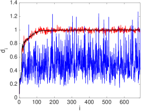
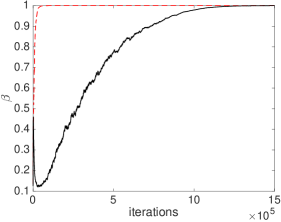
Discussion: A common criticism faced by infinite dimensional samplers is that for the purpose of applications, one must revert to a finite dimensional approximation, thus possibly defeating the purpose of proposing an infinite dimensional sampler. We counter this criticism by showing the convergence of $\beta$, and the estimate of $d$, in $\text{pCN}_{\text{AM}}$ for the truncated and the untruncated methods in Figure 1. For a fixed acceptance rate, larger value of $\beta$ implies better mixing (see [21] for instance)

Note that the final proposal distribution is almost an independence sampler, i.e., $\beta\approx 1$ which the truncated (infinite dimensional) estimator reaches in approximately $10^{4}$ iterations, and the untruncated (finite dimensional) estimator reaches in $1.5\times 10^{5}$.

Figure 1: The figure to the left shows the estimates of $d$ using the truncated estimation method (red), the untruncated estimates (blue) at the $10^{4}$th iteration, and the truncated estimates at the $10^{6}$th iteration (black). The figure at the right shows the development of $\beta$ at a fixed acceptance rate of $0.234$, for the truncated estimation method (red dashed), and the untruncated estimation method (black full).

6 Experiments

In this section, we compare many different MCMC algorithms, for three different statistical problems. The algorithms, shown in Table 1 are either developed in this article, or have been previously implemented on the problems studied here. The methods pCN_AP and pCNL_AP correspond to adapting the preconditioner by the target measure precision operator (see Section A for more details). The three examples discussed in this section are:

• A binary Gaussian classifier: This first example is taken from [21], where it was shown that the marginal auxiliary gradient sampler (mGrad) scheme preformed the best compared to a long list of other MCMC algorithms.

• Binomial likelihood with latent Matérn field: We choose this example for two specific reasons: First, using the SPDE method for the latent field allows testing the second order method involving the Hessian. Second, it allows for sparsely observed data (fewer observations compared to the dimensionality of the prior), and choosing varying number of samples in each binomial observation. Observational sparsity implies that the hessian of log-likelihood is poorly approximated by a scaled diagonal operator, which is what the mGrad algorithm builds upon. Thus we are interested to see how the adaptive method proposed here works in this situation.

• Log-Gaussian Cox process: We choose this example since it is often used in statistics, and is difficult to make inference on. In this example we also took the chance to examine how well our proposed algorithm would work when there are unknown hyperparameters that also need to be sampled.

For all three experiments we use effective sample size (ESS), see for details [15], to compare the performance of the algorithms. We also scale $\beta$ such that the acceptance rate of the Metropolis–Hastings algorithm is $0.2$ for the methods not relying on the gradient, and $0.5$ for the other methods.

$\begin{array}[]{r!{\quad\vline\quad}rlc}\text{Method}&\lx@intercol\hfil\text{second set}\hfil\lx@intercol&\text{reference }\\ \hline\cr\text{pCN}&v&=(1-c_{\beta})u+\beta\mathcal{C}^{1/2}\xi&\text{\cite[cite]{[\@@bibref{}{cotter2013mcmc}{}{}]}}\\ \text{pCN}_{\text{AM}_{0}}&v&=(1-c_{\beta})u+\beta{\cal S}\hat{\Lambda}^{1/2}_{\star}\xi&\\ \text{pCN}_{\text{AM}}&v&=(1-c_{\beta})u+c_{\beta}\hat{m}+\beta{\cal S}\hat{\Lambda}^{1/2}_{\star}\xi&\text{Sec \ref{sec:proposals-results}}\\ \text{pCNL}_{\text{AM}}&v&=(1-c_{\beta})u+c_{\beta}\left(u-{\cal S}\hat{\Lambda}_{\star}({\cal S}^{T}{\nabla}\Phi(u)+{\cal S}^{-1}u)\right)+\beta{\cal S}\hat{\Lambda}^{1/2}_{\star}\xi&\text{Sec \ref{sec:proposals-results}}\\ \text{pCNL}_{\text{AP}}&v&={\cal S}(\mathcal{I}+C_{\beta}){\cal S}^{-1}u+{\cal S}C_{\beta}{\cal S}^{T}{\nabla}\Phi(u)+{\cal S}D_{\beta}\xi&\text{Sec \ref{sec:precondprop}}\\ \text{pCN}_{\text{AP}}&v&={\cal S}(\mathcal{I}-C_{\beta}){\cal S}^{-1}u+{\cal S}C_{\beta}{\cal S}^{-1}\hat{m}+{\cal S}D_{\beta}\xi&\text{Sec \ref{sec:precondprop}}\\ \text{pCNL}_{\text{HM}}&v&=(1-c_{\beta})u+c_{\beta}B(u)(\nabla\Phi(u)-\mathcal{C}^{-1}u)+\beta B^{1/2}(u)\xi&\text{Sec \ref{sec:proposals-results}}\\ \text{MALA}&v&=u+\frac{1}{2}\beta^{2}{\cal S}\Lambda_{\star}{\cal S}^{T}(\nabla\Phi(u)-\mathcal{C}^{-1}u)+\beta{\cal S}\hat{\Lambda}^{1/2}_{\star}\xi&\text{\cite[cite]{[\@@bibref{}{grenander1994representations}{}{}]}}\\ \text{mGrad}&v&=\frac{\delta}{2}A\left(u+\frac{\delta}{2}\nabla\Phi(u)\right)+\left(\frac{2}{\delta}A^{2}+A\right)^{1/2}\xi&\text{\cite[cite]{[\@@bibref{}{titsias2016auxiliary}{}{}]}}\\ \end{array}$

Table 1: The MCMC methods used in the experiment section. The operator $A=\left(\mathcal{C}^{-1}+\frac{2}{\delta}\mathcal{I}\right)^{-1}$ and $B(u)=(\mathcal{C}^{-1}+H(u))^{-1}$. Recall that $\beta$ and $\delta$ are scaling parameters. Here $\hat{m}$ and $\hat{\Lambda}$ are estimated as shown in the reference section. The method $pCN_{AM_{0}}$ is just the adaptive measure without the posterior expectation.

Method	$\min\text{(ESS)}/s$	$\min\text{(ESS)}/\text{iter}$	$\text{median(ESS)}/s$	$\text{median(ESS)}/\text{iter}$	$\beta$
Zeroth order method
pCN	2.5	0.0004	5.0	0.0009	0.13
$\text{pCN}_{\text{AM}_{0}}$	2.5	0.0005	4.5	0.0010	0.13
$\text{pCN}_{\text{AP}}$	52.3	0.0114	66.3	0.0144	0.96
$\text{pCN}_{\text{AM}}$	215.3	0.0446	273.2	0.0565	1.00
First order method
$\text{pCNL}_{\text{AP}}$	285.9	0.0874	300.3	0.0918	0.96
$\text{pCNL}_{\text{AM}}$	341.7	0.1013	499.0	0.1479	0.92
mGrad	112.0	0.0463	254.8	0.0983	0.96

Table 2: Result of various samplers for the Australian data set. The results are generated through $300k$ iteration after $20k$ burnin. The dimension of the data is $n=690$ and $D=14$

Method	$\min\text{(ESS)}/s$	$\min\text{(ESS)}/\text{iter}$	$\text{median(ESS)}/s$	$\text{median(ESS)}/\text{iter}$	$\beta$
Zeroth order method
pCN	1.6	0.0005	3.12	0.0009	0.13
$\text{pCN}_{\text{AM}_{0}}$	0.8	0.0003	2.0	0.0007	0.11
$\text{pCN}_{\text{AP}}$	17.9	0.0073	22.1	0.0090	0.97
$\text{pCN}_{\text{AM}}$	120.7	0.0403	151.8	0.0507	1.00
First order method
$\text{pCNL}_{\text{AP}}$	162.0	0.0867	171.8	0.0917	0.97
$\text{pCNL}_{\text{AM}}$	238.7	0.1230	348.6	0.1796	0.97
mGrad	71.8	0.0475	155.4	0.1026	0.93

Table 3: Result of various samplers for the German credit dataset. The results are generated through $100k$ iteration after $20k$ burnin. The dimension of the data is $n=1000$ and $D=24$

Method	$\min\text{(ESS)}/s$	$\min\text{(ESS)}/\text{iter}$	$\text{median(ESS)}/s$	$\text{median(ESS)}/\text{iter}$	$\beta$
Zeroth order method
pCN	24.4	0.0031	31.2	0.004	0.29
$\text{pCN}_{\text{AM}_{0}}$	3.7	0.0006	8.0	0.0013	0.17
$\text{pCN}_{\text{AP}}$	216.9	0.0347	259.8	0.0416	0.97
$\text{pCN}_{\text{AM}}$	1226.1	0.1964	1646.9	0.2638	1.00
First order method
$\text{pCNL}_{\text{AP}}$	552.5	0.1364	566.1	0.1393	0.96
$\text{pCNL}_{\text{AM}}$	874.7	0.2048	1368.1	0.3203	1.00
mGrad	344.8	0.0887	841.3	0.1026	0.97

Table 4: Result of various samplers for the Pima Indian dataset. The results are generated through $100k$ iteration after $20k$ burnin. The dimension of the data is $n=532$ and $D=7$

Method	$\min\text{(ESS)}/s$	$\min\text{(ESS)}/\text{iter}$	$\text{median(ESS)}/s$	$\text{median(ESS)}/\text{iter}$	$\beta$
Zeroth order method
pCN	14.8	0.0008	22.4	0.0012	0.16
$\text{pCN}_{\text{AM}_{0}}$	11.3	0.0007	46.9	0.0029	0.26
$\text{pCN}_{\text{AP}}$	80.0	0.0049	190.0	0.0117	0.94
$\text{pCN}_{\text{AM}}$	125.5	0.0075	306.3	0.182	0.63
First order method
$\text{pCNL}_{\text{AP}}$	275.1	0.0232	535.8	0.0453	0.94
$\text{pCNL}_{\text{AM}}$	275.4	0.0232	642.7	0.054	0.62
mGrad	86.4	0.0887	508.9	0.055	0.98

Table 5: Result of various samplers for the Ripley dataset. The results are generated through $100k$ iteration after $20k$ burnin. The dimension of the data is $n=250$ and $D=2$

6.1 Binary Gaussian classification

In this example we explore the performance of different algorithms on a binary Gaussian process classification model. The target density is the posterior distribution of the following model:

$$U \sim{\cal N}(0,\mathcal{C})$$

$$Y_{i} =\text{Ber}(g^{-1}(U({\boldsymbol{\mathrm{s_{i}}}}))),\,i=1,\ldots,N,$$

where $g$ is the logistic function, ${\boldsymbol{\mathrm{s}}}_{i}\in\mathbb{R}^{d}$ the location, and $\mathcal{C}$ is the Gaussian covariance operator, i.e. $\text{cov}[u({\boldsymbol{\mathrm{s_{i}}}}),u({\boldsymbol{\mathrm{s_{j}}}})]=\sigma^{2}_{x}\exp\left(-\frac{1}{2l^{2}}||{\boldsymbol{\mathrm{s_{i}}}}-{\boldsymbol{\mathrm{s_{j}}}}||\right)$. Here we test the performance of our algorithms specifically against mGrad, which was the best algorithm from the set of algorithms discussed in [21] with the target density defined above. In [21] the model was explored on a series of data sets, for instance the “Australian Credit dataset”, where $n=690$ and the input dimension (the dimension of ${\boldsymbol{\mathrm{s}}}$) is $D=14$. We fixed the latent parameters, $(\sigma_{x},l)$ to the same values as in [21].

The results of our tests are summarized in the tables 2, 3, 4 and 5 for $300k$ iterations and a burnin of $20k$. The algorithm that preforms best is clearly $\text{pCN}_{\text{AM}}$. However, it is interesting to see that $\text{pCN}_{\text{AM}}$ performs at par with the algorithms using the gradient, and even out preform them in one of the data sets. The importance of contracting to the posterior mean is clear since the $\text{pCN}_{\text{AM}_{0}}$ performed worse then the regular pCN. That $\beta$ is almost one, for $\text{pCN}_{\text{AM}}$, in many of the experiments means that the algorithm is almost equivalent to an independence sampler.

6.2 Binomial random field

In this simulated example, we explore a posterior distribution where the Gaussian prior has a sparse precision matrix and sparse Hessian. For these types of models one can use the Hessian to construct an location dependent change of measures. This gives the $\text{pCNL}_{\text{HM}}$ method that one can compare the adaptive method towards.

The model explored in this section is

$$U \sim{\cal N}(0,\sigma^{2}(\kappa^{2}-\Delta)^{\alpha})),$$

$$Y_{i} \sim\text{Bin}(n_{i},g^{-1}(U({\boldsymbol{\mathrm{s}}}_{i}))),i=1,\ldots,N,$$

where $g$ is the logit function, and each ${\boldsymbol{\mathrm{s}}}_{i}\in\mathbb{R}^{2}$. In this study, we generate $(n_{i}-1)$ from a Poisson distribution.

The latent field $U({\boldsymbol{\mathrm{s}}})$, for $s$ in a domain $D$, is a Matérn field which can be produced as the solution of the stochastic differential equation $(\kappa^{2}-\Delta)^{\frac{\alpha}{2}}U({\boldsymbol{\mathrm{s}}})=\mathcal{W}({\boldsymbol{\mathrm{s}}})$, where $\mathcal{W}({\boldsymbol{\mathrm{s}}})$ is Gaussian white noise. A numerically efficient approximation of the field, on an irregular domain $D$, is the finite element discretization method (FEM) of the field. This consists of approximating $U$ in terms of (appropriately chosen) basis functions. We use the piecewise linear basis functions $\{\phi_{i}\}$ induced by a triangulation of the domain $D$, thus enabling us to write

$$U({\boldsymbol{\mathrm{s}}})\approx\sum_{i=1}^{d}\phi_{i}({\boldsymbol{\mathrm{s}}})U_{i},$$

where, the weights, $\left(U_{1},\ldots,U_{d}\right)$, is zero mean Gaussian random variable vector with sparse precision matrix (see [12]) for further details. For this approximation scheme, the cost of computing $({\cal C}^{-1}+H(u))^{-1/2}\xi$ and $m(\cdot)$ (used in the MCMC algorithm involving the Hessian) is $\mathcal{O}(d^{3/2})$ (see [16]). Thus in this case the algorithm will scale better than the adaptive method presented here given that the matrix multiplication involves a complexity of $\mathcal{O}(d^{2})$.

Again we use ESS as the principal measure of performance, and here compare the proposed methods. From the result we observe that the $\text{pCNL}_{\text{AM}}$ outperformed the other schemes. However, $\text{pCNL}_{\text{HM}}$ has the best performance per iteration, and since it scales better then the other methods as a function of $d$ it is likely to outperform the other methods for a larger $d$. Further $\text{pCNL}_{\text{HM}}$ would work better if we also sampled the hyperparameters ($\sigma$, $\kappa$ and $\alpha$).

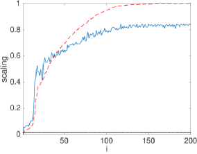
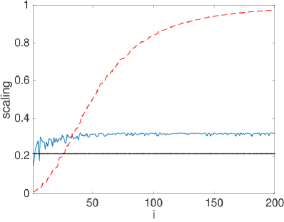
It is worth noting that the mGrad sampler performed very poorly for this model. To understand why mGrad perform so poorly, we examine what covariance operator is used to generate proposals for pCN, $\text{pCNL}_{\text{AM}}$ and mGrad. The covariance operators all have the eigenbasis of ${\cal C}$ while the scaling of the eigenvalues varies: The $i$th eigenvalue of $C$ is scaled with $\beta^{2}$ for pCN , $\delta\frac{(\delta+4\sigma_{i})}{(\delta+2\sigma^{2}_{i})}$ for mGrad and $\beta^{2}\hat{d}_{i}^{2}$ for $\text{pCNL}_{\text{HM}}$. In Figure 2, we show the scaling both for the first experiment (the Binary Gaussian process classification), where mGrad worked well, and the current examples. In the first example the mGrad eigenvalue scaling is quite similar to the scaling of $\text{pCNL}_{\text{AM}}$ which is estimated from the actual target. Whereas in the current example the mGrad and the $\text{pCNL}_{\text{AM}}$ are very different which explains the poor performance of the mGrad.

Figure 2: The figure to the left is the scaling of the eigenvalues of the proposal for Binary Classification and the Binomial distribution to the right. The red dashed line is the scaling for the auxiliary marginal, the blue full line is the scaling for $\text{pCNL}_{\text{AM}}$ and the dotted black line is for the pCN. Both figures are generated by sampling 100k samples.

Method	$\min\text{(ESS)}/s$	$\min\text{(ESS)}/\text{iter}$	$\text{median(ESS)}/s$	$\text{median(ESS)}/\text{iter}$	$\beta$
Zeroth order method
pCN	0.5	0.0001	2.0	0.0005	0.10
$\text{pCN}_{\text{AM}}$	1.5	0.004	4.5	0.0014	0.18
First order method
$\text{pCNL}_{\text{AM}}$	5.4	0.0024	14.5	0.006	0.24
mGrad	0.3	0.0006	4.3	0.009	0.70
Second order method
$\text{pCNL}_{\text{HM}}$	5.2	0.024	6.0	0.028	0.49

Table 6: Result of various samplers for the binomial Gaussian processes data. The results are generated through $10^{5}$ iteration after $20k$ burnin.

6.3 Log–Gaussian Cox processes

In this experiment we examine the performance of our algorithms within a Metropolis Hastings within Gibbs algorithm. The model is a log-Gaussian Cox process, with two hyperparameters. The data is taken from [20] and is about cases of definite or probable primary bilary cirrhosis (PBC) alive between 1987 and 1994 in Newcastle. The model is defined as follows:

$$\log(\sigma) \sim{\cal N}(0,1.5),$$

$$\log(\tau) \sim{\cal N}(10,1.5),$$

$$U({\boldsymbol{\mathrm{s}}}) \sim{\cal N}(0,\mathcal{C}_{\sigma,\tau}),$$

$$Y({\boldsymbol{\mathrm{s}}}_{i}) \sim\text{Poisson}(\exp(U({\boldsymbol{\mathrm{s}}}_{i})))\,\,\,\,\,\,\text{for}\,\,\,i=1,\ldots,N$$

Here $\mathcal{C}_{\sigma,\tau}$ is an exponential covariance operator, where $\sigma$ is the standard deviation of the field and $\tau$ the length-scale parameter. The choice of prior is identical to the one used in [20].

We are interested in examining the sampling of $\theta=\{\sigma,\tau\}$ and $U$. Although we tested both, Gibbs sampling and joint sampling, since using Gibbs sampling was computationally more efficient, we shall focus on the Gibbs sampling approach, and choose not to report the other approach. We compare three different algorithms $\text{pCNL}_{\text{AM}}$, $\text{pCN}_{\text{AM}}$ and MALA. The reason we included the regular MALA, even though it does not work in an infinite dimensional setting, is that this is what is used in the lgcp package and thus in [20]. We don’t use the package lgcp MCMC method directly due to that is an R package and thus an performance comparison would not be fair. Further, it should also be noted that in the package they are using a different scaling matrix and joint sampling (of $\theta$ and $U$) so the method can not be compared directly.

One interesting point in this experiment is that we use discrete cosine transform [17] to calculate all vector matrix product involving $\mathcal{C}_{\theta}$ which allows for efficient sampling and evaluation of the random fields. The proposed adaptive MCMC algorithms fit perfectly in here and they can be applied without compromising computational complexity.

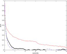
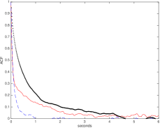
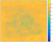
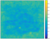
In order to test the algorithm we run them for $10^{5}$ iterations, and through Figure 4 we summarise our findings about the autocorrelation function for the entire field, $U({\boldsymbol{\mathrm{s}}})$. Here we see that the gradient methods outperform $\text{pCN}_{\text{AM}}$, however not by much. In Figure 3 we plot autocorrelation as a function of time, and it is clearly seen that the $\text{pCNL}_{\text{AM}}$ outperforms the other methods.

Figure 3: The figures shows the auto correlation as a function of run time of the algorithm. The figure to the left is for $\sigma$, and to the right is for $\tau$. The full red line is $\text{pCN}_{\text{AM}}$ , the dashed blue line is $\text{pCNL}_{\text{AM}}$ , and the dotted black line is for $MALA$.

$ACF(50)$

$\text{pCN}_{\text{AM}}$

$MALA$

$\text{pCNL}_{\text{AM}}$

$ACF(250)$

Figure 4: The top figures is the $ACF(50)$ (the autocorrelation function) for the entire latent field, the bottom figures is the same $ACF(250)$. The two figures on the left is the $\text{pCN}_{\text{AM}}$, the middle figures are the MALA and the figures to the right is $\text{pCNL}_{\text{AM}}$.The average $ACF(50)$ for the methods where $0.78$ for $\text{pCN}_{\text{AM}}$, $0.38$ for MALA, and $0.08$ for $\text{pCNL}_{\text{AM}}$.

7 Discussion

In this article we studied how several adaptive Monte Carlo Markov chain methods based on Crank-Nicolson methods greatly improve performance of their non adaptive counterparts for Gaussian processes. We have further shown that regular estimation method used in finite dimensional setting can not be used in the infinite dimensional adaptive MCMC schemes. We have also shown that using the posterior mean as a replacement for the gradient when it is not available can bring immense improvement in convergence of sampling schemes, and sometimes even outperforms the methods employing the gradient.

We would like to point at few interesting research direction that we feel are worth exploring.

• The first is extending the method here to allow choosing ${\cal K}$ from a more general class of operators, possibly not diagonalisable in the same basis as that of ${\cal C}$, thereby introducing dependence between the Karhunen–Loéve coefficients, and thus widening the applicability of our schemes. It seems likely that estimating a few correlation coefficient or some partial correlations (like in [22]) could greatly improve mixing, and the ordering of the eigenvalues give a natural path to choose which correlation coefficient that could be allowed to be non-zero. One type of model where this would be epically interesting is level sets models [9, 5]. For these models the gradient does not contribute towards convergence of the MCMC sampler, and thus the samplers which do no include the gradient, like $\text{pCN}_{\text{AM}}$ should have great potential if one can find the appropriate basis (it is not the Karhunen–Loéve basis).

• The second direction is the scaling of various block of parameters in the joint proposal. We were unable to get the performance of the joint sampling to work satisfactorily in the final experiment due to this precise issue, however it seems that in many situations the joint sampling should outperform the Gibbs sampling.

• Finally, as discussed in Section 2.3, the specific choice of ordering in the Kullback–Leibler divergence allowed for ready implementability of the optimisation scheme for choosing the parameters involved in the proposal step. It is worth investigating the optimality criterion when using the alternate ordering in the KL divergence as suggested in [14].

Appendix A Preconditioning

An alternative to change the base measure is to just adapt the preconditioner, $\mathcal{K}$, used for pCN and pCNL. That results in setting ${\cal K}={\cal S}\Lambda_{\star}{\cal S}^{T}$ while keeping ${\cal L}={\cal C}^{-1}$. For these two algorithm we get the algorithms described below.

A.1 The proposals

A.2 Preconditioning: the analysis

Here we shall present the details of the analysis involved in putting forth the proposals mentioned above. Starting with pCNL , we replace the gradient in the term with the scaled mean of target distribution, and thus generate two more algorithms bearing striking resemblance to the regular pCN .

Recall, in the SPDE (4) one can choose ${\cal K}$ to be any positive linear operator, and the usual discretization of the above SPDE with $\gamma=1$, yielded

$$v=\left(2{\cal I}+\delta{\cal K}{\cal L}\right)^{-1}\,\left[\left(2{\cal I}-\delta{\cal K}{\cal L}\right)\,u-2\delta{\cal K}{\nabla}\Phi(u)+\sqrt{8{\cal K}\,\delta}\,\xi\right]$$ (25)

As stated earlier, ${\cal L}$ is set to equal ${\cal C}^{-1}$ when discussing pCN and pCNL. We shall incorporate the Gaussian parameters as discussed in the previous section into the proposal distribution of thus generated Markov chain.

Notice now that the operator ${\cal K}$ is a free parameter, and thus can be modulated to reflect the information gained from the previous section. In particular, we could set ${\cal K}={\cal C}^{1/2}\Lambda_{\star}{\cal C}^{T/2}$, where $\Lambda_{\star}$ is as defined earlier. Such a choice of ${\cal K}$ enables Thus, in the eigenbasis of ${\cal C}$, the proposal (25) can be restated as

$$v_{i}=\left(1-\beta^{2}_{i}\right)^{1/2}u_{i}-\left(1-\left(1-\beta^{2}_{i}\right)^{1/2}\right)\sigma_{i}\,\left[{\nabla}\Phi(u)\right]_{i}+\beta_{i}\sigma_{i}^{1/2}\xi_{i}$$

where $\xi\sim{\cal N}(0,1)$; $\{\sigma_{i}\}_{i\geq 1}$ and $\{d_{\star,i}\}_{i\geq 1}$ are the eigen values of ${\cal C}$ and $\Lambda_{\star}$, respectively, and $\beta^{2}_{i}=\frac{8\delta\,d_{\star,i}}{(2+\delta d_{\star,i})^{2}}$.

One can derive that the corresponding Metropolis hasting ratio for the proposal is given by

$$\mathcal{J}(v,u)= \Phi(u)-\Phi(v)+\frac{\delta}{4}\sum_{i\geq 1}(v_{i}+u_{i})\left(\left[{\nabla}\Phi(u)\right]_{i}-\left[{\nabla}\Phi(v)\right]_{i}\right)+$$

$$\frac{\delta}{4}\sum_{i\geq 1}d_{\star,i}\left(\left[{\nabla}\Phi(u)\right]^{2}_{i}-\left[{\nabla}\Phi(v)\right]^{2}_{i}\right)+\frac{1}{2}\sum_{i\geq 1}(v_{i}-u_{i})\left(\left[{\nabla}\Phi(u)\right]_{i}+\left[{\nabla}\Phi(v)\right]_{i}\right).$$

Appendix B Karhunen–Loéve Implementing the schemes

In practice, when writing code, it is easier to encode the algorithms in terms of the Karhunen–Loéve coefficients, $z_{u}={\cal S}^{-1}u$. If using a fixed prior with no hyper parameters, it is equivalent to use $z_{u}$ or $u$ in sampling. As a template, we shall state the algorithm for sampling the Karhunen–Loéve components for $\text{pCNL}_{\text{AM}}$ only, and leave the Karhunen–Loéve component versions of other proposals to the reader.

References

- [1] A. Apte, M. Hairer, A. M. Stuart, and J. Voss. Sampling the posterior: an approach to non-Gaussian data assimilation. Phys. D, 230(1-2):50–64, 2007.
- [2] J. E. Besag. Comments on ”representations of knowledge in complex systems”, by U. Grenander and M. I. Miller. J. Roy. Statist. Soc. Ser. B Stat. Methodol., 56(4):591–592, 1994.
- [3] A. Beskos, G. Roberts, A. M. Stuart, and J. Voss. MCMC methods for diffusion bridges. Stochastics and Dynamics, 8(3):319–350, 2008.
- [4] S. L. Cotter, G. O. Roberts, A. M. Stuart, D. White, et al. MCMC methods for functions: modifying old algorithms to make them faster. Statistical Science, 28(3):424–446, 2013.
- [5] M. M. Dunlop, M. A. Iglesias, and A. M. Stuart. Hierarchical Bayesian level set inversion. Statistics and Computing, 27(6):1555–1584, 2017.
- [6] Z. Feng and J. Li. An adaptive independence sampler MCMC algorithm for infinite dimensional bayesian inferences. SIAM J. Sci. Comput., In press.
- [7] P. J. Green, K. Ł atuszyński, M. Pereyra, and C. P. Robert. Bayesian computation: a summary of the current state, and samples backwards and forwards. Stat. Comput., 25(4):835–862, 2015.
- [8] H. Haario, E. Saksman, and J. Tamminen. An adaptive Metropolis algorithm. Bernoulli, 7(2):223–242, 2001.
- [9] A. Hildeman, D. Bolin, J. Wallin, and J. B. Illian. Level set cox processes. to appear in Spatial statistics, 2018.
- [10] H.-H. Kuo. Gaussian Measures in Banach Spaces. Number 463 in Lecture Notes in Mathematics. Springer-Verlag, 1970.
- [11] K. J. H. Law. Proposals which speed up function-space MCMC. J. Comput. Appl. Math., 262:127–138, 2014.
- [12] F. Lindgren, H. Rue, and J. Lindström. An explicit link between Gaussian fields and Gaussian Markov random fields: the stochastic partial differential equation approach. Journal of the Royal Statistical Society: Series B (Statistical Methodology), 73(4):423–498, 2011.
- [13] F. J. Pinski, G. Simpson, A. M. Stuart, and H. Weber. Algorithms for Kullback–Leibler approximation of probability measures in infinite dimensions. SIAM J. Sci. Comput., 37(6):2733–2757, 2015.
- [14] F. J. Pinski, G. Simpson, A. M. Stuart, and H. Weber. Kullback–Leibler approximation for probability measures on infinite dimensional spaces. SIAM J. Mathematical Analysis, 47(6):4091–4122, 2015.
- [15] C. Robert and G. Casella. Monte Carlo Statistical Methods. Springer Texts in Statistics. Springer New York, 2013.
- [16] H. Rue and L. Held. Gaussian Markov Random Fields: Theory and Applications. London: Chapman and Hall-CRC Press, 2005.
- [17] G. Strang. The discrete cosine transform. SIAM review, 41(1):135–147, 1999.
- [18] A. M. Stuart. Inverse problems: a Bayesian perspective. Acta Numerica, 19:451–559, 2010.
- [19] A. M. Stuart, J. Voss, and P. Wiberg. Fast communication conditional path sampling of SDEs and the Langevin MCMC method. Commun. Math. Sci., 2(4):685–697, 2004.
- [20] B. Taylor, T. Davies, B. Rowlingson, and P. Diggle. Bayesian inference and data augmentation schemes for spatial, spatiotemporal and multivariate log-Gaussian Cox processes in r. Journal of Statistical Software, 63:1–48, 2015.
- [21] M. K. Titsias and O. Papaspiliopoulos. Auxiliary gradient-based sampling algorithms. arXiv preprint arXiv:1610.09641, 2016.
- [22] J. Wallin and D. Bolin. Efficient adaptive mcmc through precision estimation. to appear in journal of computational and statistical graphics, 2018.
- [23] Q. Zhou, Z. Hu, Z. Yao, and J. Li. A hybrid adaptive MCMC algorithm in function spaces. SIAM J. Uncertainty Quantification, 5:621–639, 2017.