Semileptonic $B_{(s)}\to a_{1}(K_{1})\ell^{+}\ell^{-}$ decays via the light-cone sum rules with $B$-meson distribution amplitudes

Abstract

The form factors of semileptonic $B_{(s)}\to a_{1}(K_{1})\,\ell^{+}\ell^{-}$, $\ell=\tau,\mu,e$ transitions are investigated in the framework of the light-cone sum rules with $B$-meson distribution amplitudes, which play an important role in exclusive $B$ decays. The $B$-meson distribution amplitudes, $\varphi_{\pm}(\omega)$ are a model-dependent form, so we consider four different parameterizations which can provide a reasonable description of $\varphi_{\pm}(\omega)$ from QCD corrections. The branching fractions of these transitions are calculated. For a better analysis, a comparison of our results with the prediction of other models is provided.

I Introduction

Inclusive and exclusive decays of $B$-meson play a perfect role in determination of fundamental parameters used in the standard model (SM) and improve our studies in understanding the dynamics of quantum chromo dynamics (QCD). Among of all $B$ decays, the semileptonic decays occupy a special place since their theoretical description is relatively simple. In this field, reliable calculations of heavy-to-light transition form factors of semileptonic $B$ decays are very important in particle physics. These form factors are also used to determine the amplitude of non-leptonic $B$ decays applied to evaluate the CKM parameters as well as to test various properties of the SM.

In the region of large momentum transfer squared, ($q^{2}$) heavy-to-light form factors are successfully investigated via the Lattice QCD. But in small $q^{2}$, other approaches are used such as the light-cone sum rules (LCSR) Kolesnichenko ; Halperin ; Zhitnitsky . In the usual LCSR method, the correlation function is inserted between the vacuum and light meson. As a result of this calculation, the long distance dynamics is described by light-cone distribution amplitudes (LCDA’s) of light meson Ruckl ; Simma ; Belyaev ; Weinzierl ; Bagan ; Ball ; Zwicky ; BZwicky ; BBraun . Still, there is very limited knowledge of the nonperturbative parameters determining these LCDA’s. Therefore, the main uncertainty in estimating the form factors comes from the limited accuracy of the LCDA parameters.

As the direct analogue of the LCDA’s of light mesons, the $B$-meson distribution amplitudes (DA’s) were introduced to describe generic exclusive $B$ decays with the contribution of the hard gluon exchange Brodsky . Based on the local OPE and condensate expansion, the classical two-point sum rules was used for the $B$-meson DA’s already in the original study Grozin . The $B$-meson DA’s emerge as universal nonperturbative objects in many studies of exclusive $B$-meson decays (for instance see Beneke ). An estimate of the inverse moment of two-particle DA, $\varphi_{+}$ was also obtained by matching the factorization formula to the LCSR for $B\to\gamma\ell\nu$ Kou . The shapes of the $B$-meson DA, $\varphi_{+}$ depends on the model and our knowledge of the behaviors of $\varphi_{+}$ is still rather limited due to the poor understanding of nonperturbative QCD dynamics.

Using the LCSR technique and relating the $B$-meson DA’s to the $B\to\pi$ form factor, a new approach was suggested in Offen . In this new LCSR, correlation function was taken between the vacuum and $B$-meson and it was expanded in terms of $B$-meson DA’s near the light-cone region. Therefore, the link was established between the $B$-meson DA’s and transition form factors, which provide an independent dynamical information on the $B$-meson DA’s. The new LCSR has been derived for $B\to\pi,K$ and $B\to\rho,K^{*}$ form factors in the leading order including the contributions of two- and three-particle DA’s in Mannel . Moreover, in this reference the $B$-meson three-particle DA’s have been investigated and their form have been established at small momenta of light-quark and gluon.

In this paper the heavy-to-light decays, $B_{(s)}\to a_{1}(K_{1})\,\ell^{+}\ell^{-},\ell=e,\mu,\tau$ are described by the flavor changing neutral current (FCNC) processes via $b\to d\,\ell^{+}\ell^{-}$ transition at quark level which proceed through the electroweak penguin and box diagrams. The exclusive FCNC $B$ decays are important for development of new physics and flavor physics beyond the SM. The main purpose of this paper is to consider the form factors of the FCNC $B_{(s)}\to a_{1}(K_{1})$ transition with LCSR approach, using the $B$-meson DA’s, and comparing these form factors with those of other approaches, especially the usual LCSR. Comparing form factor results between two independent methods establish input parameters and assumptions as well as predictions of the conventional LCSR.

It should be noted that the physical state of $K_{1}(1270)$ meson is consider as a mixture of two $|^{3}P_{1}\rangle$ and $|^{1}P_{1}\rangle$ states and can be parameterized in terms of a mixing angle $\theta_{K}$, as follows Hatanaka :

$$|K_{1}(1270)\rangle = \sin\theta_{K}|^{3}P_{1}\rangle~{}+\cos\theta_{K}|^{1}P_{1}\rangle,$$ (1)

where $|^{3}P_{1}\rangle\equiv|K_{1A}\rangle$ and $|^{1}P_{1}\rangle\equiv|K_{1B}\rangle$ with different masses and decay constants. Also $\theta_{K}$ is the mixing angle and can be determined by the experimental data. There are various approaches to estimate the mixing angle. In Burakovsky the result $35^{\circ}<|\theta_{K}|<55^{\circ}$ was found while in  Suzuki , two possible solutions with $|\theta_{K}|\approx 33^{\circ}$ and $57^{\circ}$ were obtained.

The contents of this paper are as follows: In section II, the effective weak Hamiltonian of the $b\to d~{}\ell^{+}\ell^{-}$ transition are presented. In section III, we derive the $B_{(s)}\to a_{1}(K_{1})\,\ell^{+}\ell^{-}$ form factors with the LCSR method using the $B$-meson DA’s. To achieve a better analysis, we consider four different parameterizations for the shapes of the $B$-meson DA’s, $\varphi_{\pm}$. The form factors of the $B_{(s)}\to a_{1}(K_{1})\,\ell^{+}\ell^{-}$ decays are basic parameters in studying the exclusive non-leptonic two-body decays and semileptonic decays. Our numerical analysis of the form factors as well as branching ratio values and their comparison with the prediction of other approaches is provided in section IV.

II The effective weak Hamiltonian of the $b\to d~{}\ell^{+}\ell^{-}$ transition

In the SM, the $B_{(s)}\to a_{1}(K_{1})\,\ell^{+}\ell^{-}$ decay amplitude is reduced to the matrix element defined as $\langle a_{1}(K_{1})\,\ell^{+}\ell^{-}|\mathcal{H}^{b\to d}_{\rm eff}|B_{(s)}\rangle.$ The effective weak Hamiltonian of the $b\to d~{}\ell^{+}\ell^{-}$ transition has the following form in the SM:

$$H^{b\to d}_{\rm eff}=-\frac{G_{F}}{\sqrt{2}}\left(V_{ub}V_{ud}^{*}\sum_{i=1}^{2}C_{i}(\mu)O^{u}_{i}(\mu)+V_{cb}V_{cd}^{*}\sum_{i=1}^{2}C_{i}(\mu)O^{c}_{i}(\mu)-V_{tb}V_{td}^{*}\sum_{i=3}^{10}C_{i}(\mu)O_{i}(\mu)\right),$$ (2)

where $V_{jk}$ and $C_{i}(\mu)$ are the CKM matrix elements and Wilson coefficients, respectively. The local operators are current-current operators $O^{u,c}_{1,2}$, QCD penguin operators $O_{3-6}$, magnetic penguin operators $O_{7,8}$, and semileptonic electroweak penguin operators $O_{9,10}$. The explicit expressions of these operators for $b\to d\ell^{+}\ell^{-}$ transition are written as Buras0

$$\begin{array}[]{ll}O_{1}=(\bar{d}_{i}c_{j})_{V-A},(\bar{c}_{j}b_{i})_{V-A},&O_{2}=(\bar{d}c)_{V-A}(\bar{c}b)_{V-A},\\ O_{3}=(\bar{d}b)_{V-A}\sum_{q}(\bar{q}q)_{V-A},&O_{4}=(\bar{d}_{i}b_{j})_{V-A}\sum_{q}(\bar{q}_{j}q_{i})_{V-A},\\ O_{5}=(\bar{d}b)_{V-A}\sum_{q}(\bar{q}q)_{V+A},&O_{6}=(\bar{d}_{i}b_{j})_{V-A}\sum_{q}(\bar{q}_{j}q_{i})_{V+A},\\ O_{7}=\frac{e}{8\pi^{2}}m_{b}(\bar{d}\sigma^{\mu\nu}(1+\gamma_{5})b)F_{\mu\nu},&O_{8}=\frac{g}{8\pi^{2}}m_{b}(\bar{d}_{i}\sigma^{\mu\nu}(1+\gamma_{5}){T}_{ij}b_{j}){G}_{\mu\nu},\\ O_{9}=\frac{e}{8\pi^{2}}(\bar{d}b)_{V-A}(\bar{l}l)_{V},&O_{10}=\frac{e}{8\pi^{2}}(\bar{d}b)_{V-A}(\bar{l}l)_{A},\end{array}$$ (8)

where ${G}_{\mu\nu}$ and $F_{\mu\nu}$ are the gluon and photon field strengths, respectively; ${T}_{ij}$ are the generators of the $SU(3)$ color group; $i$ and $j$ denote color indices. Labels $(V\pm A)$ stand for $\gamma^{\mu}(1\pm\gamma^{5})$. The magnetic and electroweak penguin operators $O_{7}$, and $O_{9,10}$ are responsible for the short distance (SD) effects in the FCNC $b\to d$ transition, but the operators $O_{1-6}$ involve both SD and long distance (LD) contributions in this transition. In the naive factorization approximation, contributions of the $O_{1-6}$ operators have the same form factor dependence as $C_{9}$ which can be absorbed into an effective Wilson coefficient $C^{\rm eff}_{9}$. Therefore, the matrix element for the $b\rightarrow d\ell^{+}\ell^{-}$ transition can be written as:

$$\cal{M} = \frac{G_{F}\alpha}{2\sqrt{2}\pi}V_{tb}V_{td}^{*}\Bigg{[}C_{9}^{\rm eff}\overline{d}\gamma_{\mu}(1-\gamma_{5})b~{}\overline{l}\gamma_{\mu}l+C_{10}\overline{d}\gamma_{\mu}(1-\gamma_{5})b~{}\overline{l}\gamma_{\mu}\gamma_{5}\l$$ (9)

$$- 2C_{7}^{\rm eff}\frac{m_{b}}{q^{2}}\overline{d}~{}i\sigma_{\mu\nu}q^{\nu}(1+\gamma_{5})b~{}\overline{l}\gamma_{\mu}l\Bigg{]},$$

where $\bar{d}\gamma_{\mu}(1-\gamma_{5})b$ and $\bar{d}\,i\sigma_{\mu\nu}q^{\nu}(1+\gamma_{5})b$ are the transition currents denoted with $J^{V-A}_{\mu}$ and $J^{T}_{\mu}$ respectively, in this work. Eq. (9) also contains two effective Wilson coefficients $C_{7}^{\rm eff}$ and $C_{9}^{\rm eff}$, where $C_{7}^{\rm eff}=C_{7}-C_{5}/3-C_{6}$. The effective Wilson coefficient $C_{9}^{\rm{eff}}$ includes both the SD and LD effects as

$$C^{\rm eff}_{9}=C_{9}+Y_{SD}(q^{2})+Y_{LD}(q^{2}),$$ (10)

where $Y_{SD}(q^{2})$ describes the SD contributions from four-quark operators far away from the resonance regions, which can be calculated reliably in perturbative theory as Buras0 ; Aliev0 :

$$Y_{SD}(q^{2}) = 0.138~{}\omega(s)+h(\hat{m_{c}},s)C_{0}-\frac{1}{2}h(1,s)(4C_{3}+4C_{4}+3C_{5}+C_{6})$$ (11)

$$- \frac{1}{2}h(0,s)(2\lambda_{u}[3C_{1}+C_{2}]+C_{3}+4C_{4})+\frac{2}{9}(3C_{3}+C_{4}+3C_{5}+C_{6}),$$

where $s=q^{2}/m_{b}^{2}$, $\hat{m_{c}}=m_{c}/m_{b}$, $C_{0}=-\lambda_{c}(3C_{1}+C_{2})+3C_{3}+C_{4}+3C_{5}+C_{6}$, $\lambda_{c}=\frac{V_{cb}V^{*}_{cd}}{V_{tb}V^{*}_{td}}$, $\lambda_{u}=\frac{V_{ub}V^{*}_{ud}}{V_{tb}V^{*}_{td}}$, and

$$\omega(s) = -\frac{2}{9}\pi^{2}-\frac{4}{3}{\rm Li}_{2}(s)-\frac{2}{3}\ln(s)\ln(1-s)-\frac{5+4s}{3(1+2s)}\ln(1-s)-\frac{2s(1+s)(1-2s)}{3(1-s)^{2}(1+2s)}\ln(s)$$ (12)

$$+ \frac{5+9s-6s^{2}}{3(1-s)(1+2s)},$$

represents the ${\cal O}(\alpha_{s})$ correction coming from one gluon exchange in the matrix element of the operator $O_{9}$ Jezabek , while $h(\hat{m}_{c},s)$ and $h(0,s)$ represent one-loop corrections to the four-quark operators $O_{1-6}$ Misiak . The functional form of the $h(\hat{m_{c}},s)$ and $h(0,s)$ are as:

$$h(\hat{m}_{c},s) = -\frac{8}{9}\ln\frac{m_{b}}{\mu}-\frac{8}{9}\ln\hat{m}_{c}+\frac{8}{27}+\frac{4}{9}x$$ (15)

$$- \frac{2}{9}(2+x)|1-x|^{1/2}\left\{\begin{array}[]{ll}\left(\ln\left|\frac{\sqrt{1-x}+1}{\sqrt{1-x}-1}\right|-i\pi\right),&\mbox{for }x\equiv\frac{4\hat{m}_{c}^{2}}{s}<1\\ &\\ 2\arctan\frac{1}{\sqrt{x-1}},&\mbox{for }x\equiv\frac{4\hat{m}_{c}^{2}}{s}>1,\end{array}\right.$$

$$h(0,s) = \frac{8}{27}-\frac{8}{9}\ln\frac{m_{b}}{\mu}-\frac{4}{9}\ln\ s+\frac{4}{9}i\pi.$$ (16)

The LD contributions, $Y_{LD}(q^{2})$ from four-quark operators near the $u\bar{u}$, $d\bar{d}$ and $c\bar{c}$ resonances can not be calculated from the first principles of QCD and are usually parameterized in the form of a phenomenological Breit-Wigner formula as Buras0 ; Aliev0 :

$$Y_{LD}(q^{2}) = \frac{3\pi}{\alpha^{2}}\left\{\sum_{V_{i}=\psi(1s),\psi(2s)}\frac{\Gamma(V_{i}\to l^{+}l^{-})m_{V_{i}}}{m_{V_{i}}^{2}-q^{2}-im_{V_{i}}\Gamma_{V_{i}}}-\lambda_{u}h(0,s)(3C_{1}+C_{2})\sum_{V_{i}=\rho,\omega}\frac{\Gamma(V_{i}\to l^{+}l^{-})m_{V_{i}}}{m_{V_{i}}^{2}-q^{2}-im_{V_{i}}\Gamma_{V_{i}}}\right\}.$$

III $B_{(s)}\to a_{1}(K_{1})\,\ell^{+}\ell^{-}$ form factors with the LCSR

First, we start with the two-point correlation function to compute the form factors of the $B\to a_{1}\ell^{+}\ell^{-}$ via the LCSR and then explain how to extract the $B\to K_{1}$ transition form factors. The correlation function is constructed from the transition currents $J^{V-A}_{\nu}$ and $J^{T}_{\nu}$ as follows:

$$\Pi_{\mu\nu}^{V-A~{}(T)}(p,q)=i\int{d^{4}x}~{}e^{ip.x}\langle 0|\mathcal{T}\left\{J_{\mu}^{a_{1}}(x)J_{\nu}^{V-A~{}(T)}(0)\right\}|B(P)\rangle.$$ (18)

In this definition for the correlation function, $\mathcal{T}$ is the time ordering operator, $|0\rangle$ is an appropriate ground state (usually vacuum), $J_{\mu}^{a_{1}}=\bar{u}\gamma_{\mu}\gamma_{5}d$ is the interpolating current of the axial-vector meson $a_{1}$. The external momenta of the interpolating and transition currents, $J_{\mu}^{a_{1}}$ and $J_{\nu}^{V-A~{}(T)}$, are $p$ and $q$, respectively, and $P^{2}=(p+q)^{2}=m^{2}_{B}$. The leading-order diagram for $B\rightarrow a_{1}\ell^{+}\ell^{-}$ decays is depicted in Fig. 1.

Figure 1: leading-order diagram for $B\rightarrow a_{1}\ell^{+}\ell^{-}$ decays.

According to the general philosophy of the QCD sum rules and its extension, (light-cone sum rules), the above correlation function should be calculated in two different ways. In phenomenological or physical representation, it is calculated in terms of hadronic parameters. In QCD side, it is obtained in terms of DA’s and QCD degrees of freedom. The LCSR for the physical quantities like form factors are acquired equating coefficient of the sufficient structures from both representations of the same correlation function through the dispersion relation and applying Borel transformation and continuum subtraction to suppress the contributions of the higher states and continuum.

To obtain the phenomenological representation of the correlation function, a complete set of intermediate states with the same quantum number as the current $J^{a_{1}}_{\mu}$ is inserted in Eq. (18). Isolating the pole term of the lowest axial vector $a_{1}$ meson and applying Fourier transformation, we get

$$\Pi^{V-A~{}(T)}_{\mu\nu}(p,q) = \frac{1}{p^{2}-m_{a_{1}}^{2}}\langle 0|J^{a_{1}}_{\mu}(p)|a_{1}(p)\rangle\langle a_{1}(p)|J^{V-A~{}(T)}_{\nu}|B(P)\rangle+\mbox{higher states\,.}$$ (19)

The matrix element, $\langle 0|J^{a_{1}}_{\mu}(p)|a_{1}(p)\rangle$ is defined as

$$\langle 0|J_{\mu}^{a_{1}}(0)|a_{1}(p)\rangle=f_{a_{1}}m_{a_{1}}\varepsilon_{\mu},$$ (20)

where $f_{a_{1}}$ and $\varepsilon_{\mu}$ are the leptonic decay constant and polarization vector of the axial vector meson $a_{1}$, respectively. The transition matrix element, $\langle a_{1}(p)|J^{V-A~{}(T)}_{\nu}|B(P)\rangle$, can be parameterized via Lorentz invariance and parity considerations as Colangelo :

$$\langle a_{1}(p)|J_{\mu}^{V-A}|B(P)\rangle = \epsilon_{\mu\nu\alpha\beta}\varepsilon^{*\nu}P^{\alpha}p^{\beta}\;\frac{2A(q^{2})}{m_{B}-m_{a_{1}}}-~{}i\varepsilon^{\ast}_{\mu}(m_{B}-m_{a_{1}})V_{1}(q^{2})$$

$$+ i\frac{\varepsilon^{\ast}\cdot P}{m_{B}-m_{a_{1}}}(P+p)_{\mu}V_{2}(q^{2})+~{}2im_{a_{1}}\frac{\varepsilon^{\ast}\cdot P}{q^{2}}q_{\mu}[V_{3}(q^{2})-V_{0}(q^{2})],$$

$$\langle a_{1}(p)|J_{\mu}^{T}|B(P)\rangle = 2i\epsilon_{\mu\nu\alpha\beta}\varepsilon^{*\nu}P^{\alpha}p^{\beta}\;T_{1}(q^{2})+[\varepsilon^{*}_{\mu}(m_{B}^{2}-m^{2}_{a_{1}})-~{}(\varepsilon^{*}\cdot P)(P+p)_{\mu}]\;T_{2}(q^{2})$$ (21)

$$+ (\varepsilon^{*}\cdot P)[q_{\mu}-{q^{2}\over m_{B}^{2}-m^{2}_{a_{1}}}(P+p)_{\mu}]\;T_{3}(q^{2}),$$

$q^{2}$ is the momentum transfer squared of the $Z$ boson (photon). It should be noted that $V_{0}(0)=V_{3}(0)$ and the identity $\sigma_{\mu\nu}\gamma_{5}=\frac{-i}{2}\epsilon_{\mu\nu\alpha\beta}\sigma^{\alpha\beta}(\epsilon_{0123}=1)$ implies that $T_{1}(0)=T_{2}(0)$Colangelo . Moreover, $V_{3}$ can be written as a linear combination of $V_{1}$ and $V_{2}$:

$$V_{3}(q^{2})=\frac{m_{B}-m_{a_{1}}}{2m_{a_{1}}}V_{1}(q^{2})-\frac{m_{B}+m_{a_{1}}}{2m_{a_{1}}}V_{2}(q^{2}).$$ (22)

Using Eqs. (20) and (III) in Eq. (19), and performing summation over the polarization of $a_{1}$ meson, we obtain

$$\Pi_{\mu\nu}^{V-A} = \frac{f_{a_{1}}m_{a_{1}}}{p^{2}-m_{a_{1}}^{2}}\times\left[\frac{2{A}}{m_{B}-m_{a_{1}}}(q^{2})\,\epsilon_{\mu\nu\alpha\beta}P^{\alpha}p^{\beta}-i~{}{V}_{1}(q^{2})\,(m_{B}-m_{a_{1}})\,g_{\mu\nu}\right.$$

$$+i \left.\frac{{V}_{2}(q^{2})}{m_{B}-m_{a_{1}}}\,(P+p)_{\mu}P_{\nu}-i~{}\frac{2m_{a_{1}}{V}_{0}(q^{2})}{q^{2}}\,q_{\mu}P_{\nu}\right]+\mbox{higher states}\,,$$

$$\Pi_{\mu\nu}^{T} = \frac{f_{a_{1}}m_{a_{1}}}{p^{2}-m_{a_{1}}^{2}}\times\left[2\,{T}_{1}(q^{2})\,\epsilon_{\mu\nu\alpha\beta}P^{\alpha}p^{\beta}-i~{}{T}_{2}(q^{2})\,(m_{B}^{2}-m_{a_{1}}^{2})\,g_{\mu\nu}\right.$$ (23)

$$-i \left.{T}_{3}(q^{2})\,q_{\mu}P_{\nu}\right]+\mbox{higher states}\,.$$

To calculate the form factors $A$, $V_{i}(i=0,1,2)$ and ${T}_{j}(j=1,2,3)$, we will choose the structures $\epsilon_{\mu\nu\alpha\beta}P^{\alpha}p^{\beta}$, $g_{\mu\nu}$, $(P+p)_{\mu}P_{\nu}$, $q_{\mu}P_{\nu}$, from $\Pi_{\mu\nu}^{V-A}$ and $\epsilon_{\mu\nu\alpha\beta}P^{\alpha}p^{\beta}$, $g_{\mu\nu}$, and $q_{\mu}P_{\nu}$ from $\Pi_{\mu\nu}^{T}$, respectively. For simplicity, the correlations are written as

$$\Pi_{\mu\nu}^{V-A}(p,q) = \Pi_{1}~{}g_{\mu\nu}+\Pi_{2}~{}\epsilon_{\mu\nu\alpha\beta}P^{\alpha}p^{\beta}+\Pi_{3}~{}(P+p)_{\mu}P_{\nu}+\Pi_{4}~{}q_{\mu}P_{\nu}+.....,$$

$$\Pi_{\mu\nu}^{T}(p,q) = \Pi_{1}^{{}^{\prime}}~{}g_{\mu\nu}+\Pi_{2}^{{}^{\prime}}~{}\epsilon_{\mu\nu\alpha\beta}P^{\alpha}p^{\beta}+\Pi_{3}^{{}^{\prime}}~{}q_{\mu}P_{\nu}+...~{}.$$ (24)

Now, we consider the QCD part of the correlation functions in Eq. (18) based on light-cone OPE in the heavy quark effective theory (HQET). After the transition to HQET, the correlation functions are written as Mannel :

$$\Pi_{\mu\nu}^{V-A(T)}(p,q) = \widetilde{\Pi}_{\mu\nu}^{V-A(T)}(p,\widetilde{q})+\mathcal{O}(1/m_{b}),$$ (25)

where $\widetilde{q}=q-m_{b}v$, and $v$ is the four-velocity of $B$-meson. Also up to $1/m_{b}$ corrections in HQET, the state of $B$-meson $|B(P)\rangle$, and the $b$-quark field $b(x)$ are substituted by the state $|B(v)\rangle$ and the effective field $e^{-im_{b}vx}h_{v}(x)$, respectively. Therefore, the correlation functions in the heavy quark limit, ($m_{b}\to\infty$), become:

$$\widetilde{\Pi}_{\mu\nu}^{V-A}(p,\widetilde{q}) = i\int d^{4}x~{}e^{ip.x}\langle 0|\mathcal{T}\{\bar{u}(x)\gamma_{\mu}\gamma_{5}~{}iS_{d}(x)~{}\gamma_{\nu}(1-\gamma_{5})h_{v}(0)\}|B(v)\rangle,$$

$$\widetilde{\Pi}_{\mu\nu}^{T}(p,\widetilde{q}) = i\int d^{4}x~{}e^{ip.x}\langle 0|\mathcal{T}\{\bar{u}(x)\gamma_{\mu}\gamma_{5}~{}iS_{d}(x)~{}\sigma_{\nu\eta}q^{\eta}(1+\gamma_{5})h_{v}(0)\}|B(v)\rangle.$$ (26)

From Eq. (III) a convolution of a short-distance part with the matrix element of the bilocal operator is obtained between the vacuum and $B(v)$-state as:

$$\widetilde{\Pi}_{\mu\nu}^{V-A}(p,\widetilde{q}) = i\int d^{4}x~{}e^{ip.x}\times{\left\{\gamma_{\mu}\gamma_{5}~{}iS_{d}(x)~{}\gamma_{\nu}(1-\gamma_{5})\right\}}_{\alpha\beta}\langle 0|\bar{u}_{\alpha}(x)h_{v\beta}(0)|B(v)\rangle,$$

$$\widetilde{\Pi}_{\mu\nu}^{T}(p,\widetilde{q}) = i\int d^{4}x~{}e^{ip.x}\times{\left\{\gamma_{\mu}\gamma_{5}~{}iS_{d}(x)~{}\sigma_{\nu\eta}q^{\eta}(1+\gamma_{5})\right\}}_{\alpha\beta}\langle 0|\bar{u}_{\alpha}(x)h_{v\beta}(0)|B(v)\rangle.$$ (27)

The full-quark propagator, $S_{d}(x)$ of a massless quark in the external gluon field in the Fock-Schwinger gauge is as follows:

$$S_{d}(x) = i\int\frac{d^{4}k}{(2\pi)^{4}}e^{-ik.x}\left\{\frac{\not\!k}{k^{2}}-\int^{1}_{0}dv~{}G_{\mu\nu}(vx)\left[\frac{1}{2k^{4}}\not\!k\sigma^{\mu\nu}-\frac{1}{k^{2}}vx^{\mu}\gamma^{\nu}\right]\right\}.$$ (28)

In addition, the DA’s of the $B$-meson are as Wang :

$$\langle 0|\bar{u}{{}_{\alpha}(x){h_{v\beta}(0)}}|B(v)\rangle = -\frac{if_{B}m_{B}}{4}\int^{\infty}_{0}d\omega~{}e^{-i\omega v.x}\left\{(1+\not\!v)\varphi_{{}_{+}}-\frac{\not\!x\gamma_{5}}{2vx}(\varphi_{{}_{+}}-\varphi_{{}_{-}})\right\}_{\beta\alpha},$$

$$\langle 0|\bar{u}_{\alpha}(x)G_{\lambda\rho}(ux)h_{v\beta}(0)|B(v)\rangle = \frac{f_{B}m_{B}}{4}\int_{0}^{\infty}d\omega\int_{0}^{\infty}d\xi e^{-i(\omega+u\xi)v.x}\left\{\left[(v_{\lambda}\gamma_{\rho}-v_{\rho}\gamma_{\lambda})\Big{(}\Psi_{A}-\Psi_{V}\Big{)}\right.\right.$$

$$\left.\left.-i\sigma_{\lambda\rho}\Psi_{V}-\frac{x_{\lambda}v_{\rho}-x_{\rho}v_{\lambda}}{vx}X_{A}+\frac{x_{\lambda}\gamma_{\rho}-x_{\rho}\gamma_{\lambda}}{vx}Y_{A}\right](1+\not\!v)\gamma_{5}\right\}_{\beta\alpha},$$

where Mannel :

$$\Psi_{A}(\omega,\xi) = \Psi_{V}(\omega,\xi)=\frac{\lambda_{E}^{2}}{6\omega_{0}^{4}}\,\xi^{2}\,e^{-\frac{\omega+\xi}{\omega_{0}}},$$

$$X_{A}(\omega,\xi) = \frac{\lambda_{E}^{2}}{6\omega_{0}^{4}}\,\xi(2\omega-\xi)\,e^{-\frac{\omega+\xi}{\omega_{0}}},$$

$$Y_{A}(\omega,\xi) = -\frac{\lambda_{E}^{2}}{24\omega_{0}^{4}}\,\xi(7\omega_{0}-13\omega+3\xi)\,e^{-\frac{\omega+\xi}{\omega_{0}}}.$$ (30)

Our knowledge of the behaviors of $\varphi_{\pm}(\omega)$ at small $\omega$ is still rather limited due to the poor understanding of non-perturbative QCD dynamics. To achieve a better understanding of the model dependence of $\varphi_{\pm}(\omega)$ in the sum rule analysis, we consider the following four different parameterizations for the shapes of the $B$-meson DA $\varphi_{+}$ Grozin ; Braun ; Faziophi ; Wangphi :

$$\varphi_{+,\rm I}(\omega) = \frac{\omega}{\omega_{0}^{2}}\,e^{-\omega/\omega_{0}}\,,$$

$$\varphi_{+,\rm II}(\omega) = \frac{1}{4\pi\,\omega_{0}}\,{k\over k^{2}+1}\,\left[{1\over k^{2}+1}-\frac{2(\sigma_{B}-1)}{\pi^{2}}\,\ln k\right]\,,\hskip 28.45274ptk=\frac{\omega}{1\,\,\rm GeV}\,,\,$$

$$\varphi_{+,\rm III}(\omega) = \frac{2\omega^{2}}{\omega_{0}\omega_{1}^{2}}\,e^{-(\omega/\omega_{1})^{2}}\,,\hskip 28.45274pt\omega_{1}={2\,\omega_{0}\over\sqrt{\pi}}\,,$$

$$\varphi_{+,\rm IV}(\omega) = \frac{\omega}{\omega_{0}\omega_{2}}\,{\omega_{2}-\omega\over\sqrt{\omega(2\omega_{2}-\omega)}}\,\,\theta(\omega_{2}-\omega)\,,\hskip 28.45274pt\omega_{2}={4\,\omega_{0}\over 4-\pi}\,.$$ (31)

The determination of coefficient $\omega_{0}$, which constitutes the most important theory uncertainty in the $B$-meson LCSR approach, will be discussed for each of the four models in the next section.

The corresponding expression of $\varphi_{-}(\omega)$ for each model is determined by:

$$\varphi_{-}(\omega)=\int_{0}^{1}\,{d\xi\over\xi}\,\varphi_{+}\left(\omega/\xi\right).$$ (32)

These parameterizations can provide a reasonable description of $\varphi_{\pm}(\omega)$ at small $\omega$ due to the radiative tail developed from QCD corrections.

Inserting the full propagator and $B$-meson DA’s presented in Eqs. (28) and (III), respectively, in the correlation functions (Eq. (III)), traces and then integrals should be calculated. To estimate these calculations, we have used $x_{\mu}\rightarrow i\frac{\partial}{\partial{k_{\mu}}}$. In addition to this, for terms containing a factor of $vx$ in the denominator, we have used the following trick: in order not to have any singularity at $v.x=0$, the integral of these wave functions in the absence of the exponential should cancel. Hence, for these terms only, one can write:

$$e^{i\alpha v.x}\rightarrow e^{i\alpha v.x}-1=iv.x\int_{0}^{\alpha}dk~{}e^{ikv.x},$$ (33)

and the rest of the calculation is similar to the presented one. Note that the subtracted $1$ does not contribute.

After completing the integrals and matching them with the hadronic representation below the continuum threshold $s_{0}$, through the dispersion relation and applying Borel transform with respect to the variable $p^{2}$ as:

$$B_{p^{2}}(M^{2})(\frac{1}{p^{2}-m^{2}})^{n} = \frac{(-1)^{n}}{\Gamma(n)}\frac{e^{-\frac{m^{2}}{M^{2}}}}{(M^{2})^{n}},$$ (34)

in order to suppress the contributions of the higher states, the form factors are obtained via the LCSR. For instance, the form factor $V_{1}$ is presented here:

$$V_{1}(q^{2}) = -\frac{f_{B}m_{B}}{f_{a}m_{a_{1}}(m_{B}-m_{a_{1}})}e^{\frac{m_{a_{1}}^{2}}{M^{2}}}\left\{\int_{0}^{\sigma_{0}}d\sigma\left[\frac{M^{2}}{2}\varphi_{{}_{+}}(\omega^{{}^{\prime}})\frac{d}{d\sigma}e^{-\frac{s}{M^{2}}}\right]\right.+\hat{\mathcal{L}}\left[(1-u)\Psi_{{}_{V}}~{}\frac{d}{d\sigma}e^{-\frac{s}{M^{2}}}\right.$$ (35)

$$- \frac{2u-1}{2M^{2}}(\Psi_{{}_{A}}-\Psi_{{}_{V}})~{}\frac{d}{d\sigma}e^{-\frac{s}{M^{2}}}+\frac{m_{B}^{2}(1-2u)}{\bar{\sigma}^{2}{M^{2}}}(3\widetilde{X}_{{}_{A}}-\widetilde{Y}_{{}_{A}})~{}e^{-\frac{s}{M^{2}}}+\frac{1}{\bar{\sigma}^{3}M^{2}}\widetilde{X}_{{}_{A}}~{}e^{-\frac{s}{M^{2}}}$$

$$\times \left.\left.\left(m_{B}^{2}(1+3\sigma)-2\widetilde{m}{{}_{B}^{2}}+\frac{\mathcal{M}^{4}}{2M^{2}}\right)\right]\right\},$$

The explicit expressions for the other form factors are presented in Appendix.

Finally, with a little bit of change in the previous steps, such as the change in the quark spectator ($u\to s$), we can easily find similar results for the form factors of the $B_{s}\to K_{1A}$, and $B_{s}\to K_{1B}$ decays.

The form factors of $B_{s}\to K_{1}(1270)\ell^{+}\ell^{-}$ transitions with the mixing angle $\theta_{K}$ are defined as Hua

$$f^{K_{1}(1270)} = C_{1}\,\sin\theta_{K}\,f^{K_{1A}}+C_{2}\,\cos\theta_{K}\,f^{K_{1B}},$$ (36)

where $f^{K_{1}(1270)},f^{K_{1A}}$ and $f^{K_{1B}}$ stand for the form factors $A,V_{i}(i=0,1,2),T_{j}(j=1,2,3)$ of $B_{s}\to K_{1}(1270),B_{s}\to K_{1A}$ and $B_{s}\to K_{1B}$ decays, respectively. The coefficients $C_{1}$ and $C_{2}$ related to each form factor of $B_{s}\to K_{1}(1270)$ decay are given in Table 1.

Table 1: The coefficients $C_{1}$ and $C_{2}$ for each form factor of $B_{s}\to K_{1}(1270)$ .

Form factors	$C_{1}$	$C_{2}$
$A,V_{1},V_{2}$	$\frac{m_{B_{s}}-m_{K_{1}}}{m_{B_{s}}-m_{K_{1A}}}$	$\frac{m_{B_{s}}-m_{K_{1}}}{m_{B_{s}}-m_{K_{1B}}}$
$V_{0}$	$\frac{m_{K_{1A}}}{m_{K_{1}}}$	$\frac{m_{K_{1B}}}{m_{K_{1}}}$
$T_{1},T_{3}$	$1$	$1$
$T_{2}$	$\frac{{m_{B_{s}}^{2}}-m_{K_{1A}}^{2}}{m_{B_{s}}^{2}-m_{K_{1}}^{2}}$	$\frac{m_{B_{s}}^{2}-m_{K_{1B}}^{2}}{m_{B_{s}}^{2}-m_{K_{1}}^{2}}$

IV Numerical Analysis

In this section, our numerical analysis of the form factors $A$, $V_{i}$ and $T_{j}$ are presented for the $B_{(s)}\to a_{1}(K_{1})\ell^{+}\ell^{-}$ decays. The values are chosen for masses in GeV as $m_{B}=(5.27\pm 0.01)$, $m_{a_{1}}=(1.23\pm 0.04)$, $m_{K_{1}}=(1.27\pm 0.01)$, $m_{\mu}=0.11$ and $m_{\tau}=1.77$ pdg , $m_{K_{1A}}=(1.31\pm 0.06)$, $m_{K_{1B}}=(1.34\pm 0.08)$ Yang . The leptonic decay constants are taken as: $f_{a_{1}}=(0.24\pm 0.01)\,\mbox{GeV}$, $f_{K_{1A}}=(0.25\pm 0.01)\,\mbox{GeV}$, $f_{K_{1B}}=(0.19\pm 0.01)\,\mbox{GeV}$ Yang , $f_{B}=(0.18\pm 0.02)\,\mbox{GeV}$ Wan , and $f_{B_{s}}=(0.23\pm 0.03)\,\mbox{GeV}$ Li2 . Moreover, $s_{0}=(2.55\pm 0.15)\,\mbox{GeV}^{2}$ is used for the continuum threshold Yang . The values of the parameters $\lambda_{E}^{2}$ and $\sigma_{B}$ of the $B$-meson DA’s are chosen as $\lambda_{E}^{2}=(0.11\pm 0.06)\,\mbox{GeV}^{2}$ Grozin and $\sigma_{B}=1.4\pm 0.4$ Braun . The Borel parameter in this article is taken as $1.5~{}\rm GeV^{2}\leq M^{2}\leq 4~{}\rm GeV^{2}$. In this region, the values of the form factors $A$, $V_{i}$ and $T_{j}$ are stable enough. The uncertainties which originated from the Borel parameter $M^{2}$ in this interval, are about $1\%$.

Having all these input values and parameters at hand, we proceed to carry out numerical calculations. As can be seen in Eq. (III), the $B$-meson DA’s, $\varphi_{\pm}$ in the four cases are related to the parameter $\omega_{0}$ whose value is depend on the model. In order to determine the parameter $\omega_{0}$ for $B\to a_{1}\ell^{+}\ell^{-}$ decay, we match the values of the form factor $A^{B\to a_{1}}$ in $q^{2}=0$, estimated with the four models of the $B$-meson DA’s $\varphi_{\pm}$, with $A^{B\to a_{1}}(0)=0.26\pm 0.09$ computed from the PQCD as a different method Li2 , and derive the values of the coefficient $\omega_{0}$ for each model. Also, taking $A^{B_{s}\to K_{1A}}(0)=0.25\pm{0.10}$ and $A^{B_{s}\to K_{1B}}(0)=0.18\pm{0.08}$ evaluated via the PQCD Li2 , and performing the same procedure as $B\to a_{1}$ decay for $B_{s}\to K_{1A}$ and $B_{s}\to K_{1B}$ transitions, the values of the parameter $\omega_{0}$ are calculated for these decays. The values of the parameter $\omega_{0}$ for three aforementioned decays are given in Table 2.

Table 2: The values of $\omega_{0}$ for each model in MeV .

Model	I	II	III	IV
$\omega_{0}\,({\rm for}~{}B\to a_{1})$	$235^{+25}_{-19}$	$246^{+28}_{-21}$	$259^{+29}_{-22}$	$217^{+20}_{-16}$
$\omega_{0}\,({\rm for}~{}B_{s}\to K_{1A})$	$254^{+27}_{-20}$	$267^{+29}_{-22}$	$281^{+33}_{-25}$	$234^{+23}_{-17}$
$\omega_{0}\,({\rm for}~{}B_{s}\to K_{1B})$	$282^{+33}_{-22}$	$298^{+34}_{-26}$	$313^{+37}_{-28}$	$259^{+23}_{-20}$

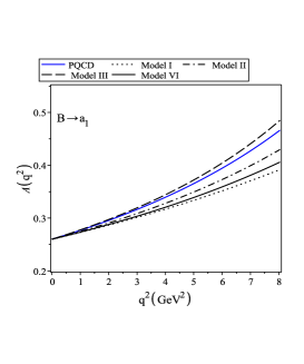
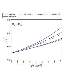
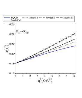
Fig. 2 shows the form factors $A^{B\to a_{1}}$, $A^{B_{s}\to K_{1A}}$ and $A^{B_{s}\to K_{1B}}$ with the four models of the $B$-meson DA’s $\varphi_{\pm}$ whose values at zero momentum transfer have been fixed to the predictions from the PQCD. In this figure, blue lines show the form factors predicted by the PQCD method.

Figure 2: Dotted, dot-dashed, dashed, solid (black) curves show the form factors $A$, calculated with the $B$-meson DA’s, whose values at $q^{2}=0$ have been fixed to the prediction from the PQCD (blue).

Now, by inserting the values of the masses, leptonic decay constants, continuum threshold, Borel mass, the parameters of the $B$-meson DA’s such as $\omega_{0}$ and other quantities that appear in the form factors, we can calculate the form factors of $B_{(s)}\to a_{1}(K_{1A},K_{1B})$ decays at zero momentum transfer. Taking into account all the uncertainties, the numerical values of the form factors $A$, $V_{i}$ and $T_{j}$ for aforementioned decays in $q^{2}=0$ are presented in Table 3 for the four models of the $B$-meson DA’s, $\varphi_{\pm}$. The main uncertainty comes from $\omega_{0}$, the decay constant $f_{a_{1}}$ $(f_{K_{1A}},f_{K_{1B}}$), and $B$-meson mass.

Table 3: The $B_{(s)}\to a_{1}(K_{1A},K_{1B})$ form factors at zero momentum transfer in the four models of $B$-meson DA’s, $\varphi_{\pm}$.

	Model	${A^{B\to a_{1}}}$	${V}^{B\to a_{1}}_{1}$	$V^{B\to a_{1}}_{2}$	$V^{B\to a_{1}}_{0}$	$T^{B\to a_{1}}_{1}=T^{B\to a_{1}}_{2}$	$T^{B\to a_{1}}_{3}$
	I	${0.26}{\pm 0.09}$	${0.42}{\pm 0.13}$	${0.22}{\pm 0.07}$	${0.11}{\pm 0.03}$	${0.25}{\pm 0.08}$	${0.22}{\pm 0.06}$
	II	${0.26}{\pm 0.09}$	${0.51}{\pm 0.16}$	${0.25}{\pm 0.08}$	${0.13}{\pm 0.04}$	${0.30}{\pm 0.09}$	${0.25}{\pm 0.07}$
	III	${0.26}\pm{0.09}$	${0.54}\pm{0.17}$	${0.28}\pm{0.09}$	${0.27}\pm{0.08}$	${0.34}\pm{0.11}$	${0.29}\pm{0.09}$
	VI	${0.26}\pm{0.09}$	${0.40}\pm{0.13}$	${0.20}\pm{0.06}$	${0.11}\pm{0.03}$	${0.24}\pm{0.07}$	${0.21}\pm{0.06}$
	Model	${A^{B_{s}\to K_{1A}}}$	${V}^{B_{s}\to K_{1A}}_{1}$	$V^{B_{s}\to K_{1A}}_{2}$	$V^{B_{s}\to K_{1A}}_{0}$	$T^{B_{s}\to K_{1A}}_{1}=T^{B_{s}\to K_{1A}}_{2}$	$T^{B_{s}\to K_{1A}}_{3}$
	I	${0.25}{\pm 0.10}$	${0.35}{\pm 0.12}$	${0.15}{\pm 0.05}$	${0.12}{\pm 0.04}$	${0.27}{\pm 0.09}$	${0.24}{\pm 0.08}$
	II	${0.25}{\pm 0.10}$	${0.37}{\pm 0.13}$	${0.18}{\pm 0.05}$	${0.11}{\pm 0.03}$	${0.32}{\pm 0.11}$	${0.27}{\pm 0.09}$
	III	${0.25}\pm{0.10}$	${0.45}\pm{0.15}$	${0.22}\pm{0.07}$	${0.12}\pm{0.04}$	${0.39}\pm{0.13}$	${0.33}\pm{0.12}$
	VI	${0.25}\pm{0.10}$	${0.33}\pm{0.11}$	${0.13}\pm{0.04}$	${0.11}\pm{0.03}$	${0.25}\pm{0.09}$	${0.21}\pm{0.07}$
	Model	${A^{B_{s}\to K_{1B}}}$	${V}^{B_{s}\to K_{1B}}_{1}$	$V^{B_{s}\to K_{1B}}_{2}$	$V^{B_{s}\to K_{1B}}_{0}$	$T^{B_{s}\to K_{1B}}_{1}=T^{B_{s}\to K_{1B}}_{2}$	$T^{B_{s}\to K_{1B}}_{3}$
	I	$0.18\pm 0.08$	$0.28\pm 0.10$	$0.12\pm 0.04$	$0.07\pm 0.02$	$0.22\pm 0.08$	$0.19\pm 0.07$
	II	$0.18\pm 0.08$	$0.33\pm 0.12$	$0.15\pm 0.05$	$0.10\pm 0.03$	$0.28\pm 0.10$	$0.25\pm 0.09$
	III	$0.18\pm 0.08$	$0.38\pm 0.14$	$0.20\pm 0.07$	$0.12\pm 0.03$	$0.33\pm 0.11$	$0.30\pm 0.11$
	VI	$0.18\pm 0.08$	$0.27\pm 0.08$	$0.11\pm 0.03$	$0.09\pm 0.02$	$0.21\pm 0.07$	$0.18\pm 0.05$

So far, several authors have calculated the form factors of the $B_{(s)}\to a_{1}(K_{1A},K_{1B})\ell^{+}\ell^{-}$ decays via differen frameworks. To compare the results, we should rescale them according to the form factor definitions in Eq. (III). Table 4 shows the values of the rescaled form factors at $q^{2}=0$ from different approaches.

Table 4: Transition form factors of the $B_{(s)}\to a_{1}(K_{1A},K_{1B})\ell^{+}\ell^{-}$ at $q^{2}=0$ in various methods.

Approaches	$A^{B\to a_{1}}$	$V^{B\to a_{1}}_{1}$	$V^{B\to a_{1}}_{2}$	$V^{B\to a_{1}}_{0}$	$T^{B\to a_{1}}_{1}=T^{B\to a_{1}}_{2}$	$T^{B\to a_{1}}_{3}$
PQCD Li2	$0.26\pm 0.09$	$0.43\pm 0.16$	$0.13\pm 0.04$	$0.34\pm 0.16$	$0.34\pm 0.13$	$0.30\pm 0.17$
LCSR mo	$0.42\pm 0.16$	$0.68\pm 0.13$	$0.31\pm 0.16$	$0.30\pm 0.18$	$0.44\pm 0.28$	$0.41\pm 0.18$
3PSR kh	$0.51$	$0.52$	$0.25$	$0.76$	$0.37$	$0.41$
	${A^{B_{s}\to K_{1A}}}$	${V}^{B_{s}\to K_{1A}}_{1}$	$V^{B_{s}\to K_{1A}}_{2}$	$V^{B_{s}\to K_{1A}}_{0}$	$T^{B_{s}\to K_{1A}}_{1}=T^{B_{s}\to K_{1A}}_{2}$	$T^{B_{s}\to K_{1A}}_{3}$
PQCD Li2	$0.25\pm 0.10$	$0.43\pm 0.19$	$0.11\pm 0.05$	$0.36\pm 0.18$	$0.34\pm 0.15$	$0.30\pm 0.13$
	${A^{B_{s}\to K_{1B}}}$	${V}^{B_{s}\to K_{1B}}_{1}$	$V^{B_{s}\to K_{1B}}_{2}$	$V^{B_{s}\to K_{1B}}_{0}$	$T^{B_{s}\to K_{1B}}_{1}=T^{B_{s}\to K_{1B}}_{2}$	$T^{B_{s}\to K_{1B}}_{3}$
PQCD Li2	$0.18\pm 0.08$	$0.33\pm 0.14$	$0.03\pm 0.03$	$0.42\pm 0.16$	$0.26\pm 0.11$	$0.17\pm 0.08$

Considering the uncertainties, our results for the form factors of these decays are in a good agreement with those of the PQCD in most cases (except $V_{2}$ and $V_{0}$). However, there is not good agreement between our results with the LCSR with $a_{1}$-meson DA’s mo .

The LCSR calculations for the form factors are truncated at about $0\leq q^{2}\leq 8{\rm GeV}^{2}$. To extend the $q^{2}$ dependence of the form factors to the full physical region, where the LCSR results are not valid, we find that the sum rules predictions for the form factors are well fitted to the following function:

$$F_{i}(q^{2})=\frac{F_{i}(0)}{1-\alpha(q^{2}/m_{B_{(s)}}^{2})+\beta{(q^{2}/m_{B_{(s)}}^{2})}^{2}},$$ (37)

where $F_{i}(0)$, $\alpha$ and $\beta$ are the constant fitted parameters. The values of the parameters $[\alpha,\beta]$ are presented in Tables 5, 6 and 7 for $B\to a_{1}$, $B_{s}\to K_{1A}$ and $B_{s}\to K_{1B}$, respectively. The values of parameter $F_{i}(0)$ expressed the form factor results at $q^{2}=0$ were listed in Table 3, before.

Table 5: The parameters $[\alpha,\beta]$ obtained for the form factors of the $B\to a_{1}$ transition in the four models.

Model	${A}(q^{2})$	${V}_{1}(q^{2})$	${V}_{2}(q^{2})$	${V}_{0}(q^{2})$	$T_{1}(q^{2})$	$T_{2}(q^{2})$	$T_{3}(q^{2})$
I	$[1.33,0.57]$	$[0.87,0.38]$	$[1.01,0.53]$	$[1.04,0.29]$	$[1.11,0.21]$	$[1.25,0.48]$	$[1.13,1.10]$
II	$[1.51,0.50]$	$[1.15,0.36]$	$[1.38,0.54]$	$[1.28,0.26]$	$[1.29,0.47]$	$[1.23,0.29]$	$[1.29,0.94]$
III	$[1.70,0.64]$	$[1.20,0.46]$	$[1.28,0.73]$	$[1.15,0.31]$	$[1.36,0.52]$	$[1.30,0.35]$	$[1.62,0.87]$
IV	$[1.34,0.46]$	$[0.88,0.30]$	$[1.03,0.42]$	$[1.08,0.22]$	$[1.41,0.17]$	$[1.31,0.38]$	$[1.14,0.88]$

Table 6: The same as Table 5 but for $B_{s}\to K_{1A}$ transition.

Model	${A}(q^{2})$	${V}_{1}(q^{2})$	${V}_{2}(q^{2})$	${V}_{0}(q^{2})$	$T_{1}(q^{2})$	$T_{2}(q^{2})$	$T_{3}(q^{2})$
I	$[1.16,0.53]$	$[0.98,0.24]$	$[1.14,0.39]$	$[0.96,0.34]$	$[1.30,0.17]$	$[1.09,0.46]$	$[0.95,1.17]$
II	$[1.44,0.56]$	$[1.31,0.32]$	$[1.20,0.49]$	$[1.25,0.34]$	$[1.34,0.28]$	$[1.33,0.35]$	$[1.08,0.91]$
III	$[1.56,0.72]$	$[1.52,0.31]$	$[1.37,0.76]$	$[1.32,0.43]$	$[1.46,0.50]$	$[1.38,0.39]$	$[1.12,0.98]$
VI	$[1.18,0.42]$	$[1.01,0.45]$	$[1.15,0.31]$	$[0.99,0.27]$	$[1.33,0.13]$	$[1.11,0.36]$	$[0.96,1.03]$

Table 7: The same as Table 5 but for $B_{s}\to K_{1B}$ transition.

Model	${A}(q^{2})$	${V}_{1}(q^{2})$	${V}_{2}(q^{2})$	${V}_{0}(q^{2})$	$T_{1}(q^{2})$	$T_{2}(q^{2})$	$T_{3}(q^{2})$
I	$[0.83,0.48]$	$[0.62,0.29]$	$[0.75,0.49]$	$[0.77,0.37]$	$[0.96,0.31]$	$[0.78,0.37]$	$[0.63,1.47]$
II	$[1.03,0.50]$	$[0.81,0.35]$	$[0.81,0.41]$	$[0.93,0.40]$	$[0.99,0.28]$	$[0.99,0.28]$	$[0.71,1.14]$
III	$[1.08,0.63]$	$[0.90,0.28]$	$[0.80,0.77]$	$[0.96,0.42]$	$[1.01,0.56]$	$[0.91,0.24]$	$[0.38,1.04]$
VI	$[0.87,0.37]$	$[0.66,0.22]$	$[0.81,0.39]$	$[0.82,0.29]$	$[0.98,0.23]$	$[0.84,0.28]$	$[0.66,1.18]$

By averaging the values of the form factors derived from the four models of the $B$-meson DA’s $\varphi_{\pm}$ at some points of $q^{2}$, and then extrapolating to the fit function in Eq. (37), we can investigate average form factors. The parameters $F_{i}(0)$, $\alpha$ and $\beta$ for the average form factors of $B_{(s)}\to a_{1}(K_{1})$ are given in Table 8. For $B_{s}\to K_{1}\ell^{+}\ell^{-}$ transition, the average form factors are calculated at $\theta_{K}=45^{\circ}$.

Table 8: The parameters $F_{i}(0),\alpha$, and $\beta$ obtained for the average form factors of the $B_{(s)}\to a_{1}(K_{1})$ transitions.

Form factor	$F_{i}(0)$	$\alpha$	$\beta$
$[A^{B\to a_{1}},A^{B_{s}\to K_{1}}]$	$[0.26,0.30]$	$[1.51,1.17]$	$[0.53,0.45]$
$[V_{1}^{B\to a_{1}},V_{1}^{B_{s}\to K_{1}}]$	$[0.46,0.48]$	$[1.05,1.43]$	$[0.36,0.16]$
$[V_{2}^{B\to a_{1}},V_{2}^{B_{s}\to K_{1}}]$	$[0.23,0.23]$	$[1.18,1.08]$	$[0.55,0.43]$
$[V_{0}^{B\to a_{1}},V_{0}^{B_{s}\to K_{1}}]$	$[0.25,0.15]$	$[1.17,1.01]$	$[0.28,0.30]$
$[T_{1}^{B\to a_{1}},T_{1}^{B_{s}\to K_{1}}]$	$[0.28,0.40]$	$[1.32,1.18]$	$[0.36,0.25]$
$[T_{2}^{B\to a_{1}},T_{2}^{B_{s}\to K_{1}}]$	$[0.28,0.40]$	$[1.29,1.08]$	$[0.38,0.27]$
$[T_{3}^{B\to a_{1}},T_{3}^{B_{s}\to K_{1}}]$	$[0.24,0.34]$	$[1.32,0.86]$	$[0.83,1.02]$

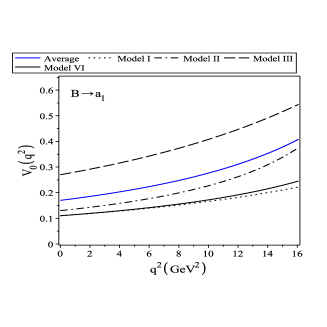
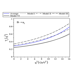
Fig. 3 show the form factors with the four models, for instance $V_{0}(q^{2})$ and $T_{1}(q^{2})$ with respect to $q^{2}$, on which blue lines display the average form factors.

Figure 3: The form factors ${V}_{0}$ and ${T}_{1}$ of $B_{(s)}\to a_{1}(K_{1})$ on $q^{2}$ with the four models (black color). Blue lines show the average form factors.

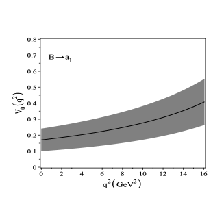
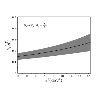
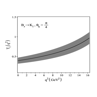
Considering the uncertainties, the average form factors $V_{0}(q^{2})$ and $T_{1}(q^{2})$ of the $B_{(s)}\to a_{1}(K_{1})$ decays with their uncertainty regions are displayed on $q^{2}$ in Fig. 4.

Figure 4: The average form factors ${V}_{0}$ and ${T}_{1}$ of $B_{(s)}\to a_{1}(K_{1})$ decays with their uncertainty regions.

Now, we are ready to evaluate the branching ratio values for the $B_{(s)}\to a_{1}(K_{1})\ell^{+}\ell^{-}$ decays. The expression of double differential decay rate ${d^{2}\Gamma}/{dq^{2}dcos\theta_{\ell}}$ for the $B_{(s)}\to a_{1}(K_{1})$ transitions can be found in Geng2 ; Colangelo . This expression contains the Wilson coefficients, the CKM matrix elements, the form factors related to the fit functions, series of functions and constants. The numerical values of the Wilson coefficients are taken from Ref. Ali . The corresponding values are listed in Table 9 in the scale $\mu=m_{b}$.

Table 9: Central values of the Wilson coefficients used in the numerical calculations.

$C_{1}$	$C_{2}$	$C_{3}$	$C_{4}$	$C_{5}$	$C_{6}$	$C_{7}^{\rm eff}$	$C_{9}$	$C_{10}$
-0.248	1.107	0.011	-0.026	0.007	-0.031	-0.313	4.344	$-4.669$

The other parameters can be found in Colangelo . After numerical analysis, the dependency of the differential branching ratios for $B\to a_{1}\ell^{+}\ell^{-}$ on $q^{2}$ using the average form factors, with and without LD effects is shown in Fig. 5 for charged lepton case.

Figure 5: The differential branching ratios of the semileptonic $B\to a_{1}(K_{1})\ell^{+}\ell^{-}$ for $\ell=\mu,\tau$ decays on $q^{2}$ with and without LD effects using the average form factors.

In Table 10, we present the branching ratio values for muon and tau without and with LD effects using the form factors derived in the four models of $\varphi_{\pm}$. We also estimate the branching ratio values with the average form factors (AFF). For $B_{s}\to K_{1}$ transitions, we have calculated the average value of branching ratios in the region $35^{\circ}<|\theta_{K}|<55^{\circ}$. Here, we should also stress that the results obtained for the electron are very close to those of the muon; and for this reason, we only present the branching ratios for muon in our table.

Table 10: Branching ratio values of the semileptonic $B_{(s)}\to a_{1}(K_{1})\ell^{+}\ell^{-}$ decays without and with LD effects using the form factors in the four models as well as the average form factors (AFF).

Only  SD  effects	model-I	model-II	model-III	model-VI	AFF
${\rm{BR}}(B\to a_{1}\mu^{+}\mu^{-})\times 10^{8}$	${2.46}\pm{0.54}$	${2.77}\pm{0.58}$	${2.96}\pm{0.62}$	${2.43}\pm{0.50}$	${2.82}\pm{0.62}$
${\rm{BR}}(B\to K_{1}\mu^{+}\mu^{-})\times 10^{8}$	${3.12}\pm{0.58}$	${3.41}\pm{0.82}$	${3.64}\pm{0.94}$	${3.09}\pm{0.57}$	${3.45}\pm{0.90}$
${\rm{BR}}(B\to a_{1}\tau^{+}\tau^{-})\times 10^{9}$	${0.23}\pm{0.05}$	${0.25}\pm{0.05}$	${0.29}\pm{0.06}$	${0.22}\pm{0.04}$	${0.27}\pm{0.06}$
${\rm{BR}}(B\to K_{1}\tau^{+}\tau^{-})\times 10^{9}$	${0.40}\pm{0.09}$	${0.44}\pm{0.10}$	${0.49}\pm{0.11}$	${0.39}\pm{0.08}$	${0.43\pm 0.10}$
SD + LD  effects	model-I	model-II	model-III	model-VI	AFF
${\rm{BR}}(B\to a_{1}\mu^{+}\mu^{-})\times 10^{8}$	${2.82}\pm{0.65}$	${3.18}\pm{0.74}$	${3.40}\pm{0.81}$	${2.79}\pm{0.64}$	${3.26}\pm{0.81}$
${\rm{BR}}(B\to K_{1}\mu^{+}\mu^{-})\times 10^{8}$	${3.80}\pm{0.83}$	${4.16}\pm{0.91}$	${4.44}\pm{0.97}$	${3.76}\pm{0.82}$	${4.24}\pm{0.95}$
${\rm{BR}}(B\to a_{1}\tau^{+}\tau^{-})\times 10^{9}$	${0.24}\pm{0.05}$	${0.26}\pm{0.05}$	${0.31}\pm{0.06}$	${0.23}\pm{0.04}$	${0.29}\pm{0.06}$
${\rm{BR}}(B\to K_{1}\tau^{+}\tau^{-})\times 10^{9}$	${0.45}\pm{0.10}$	${0.50}\pm{0.11}$	${0.54}\pm{0.12}$	${0.44}\pm{0.09}$	${0.49}\pm{0.11}$

In Ref. mo via the LCSR with $a_{1}$-meson DA’s, the branching ratio values of $B\to a_{1}\mu^{+}\mu^{-}$ and $B\to a_{1}\tau^{+}\tau^{-}$ decays by considering SD+ LD effects are predicted $(2.52\pm 0.62)\times 10^{-8}$ and $(0.31\pm 0.06)\times 10^{-9}$, respectively. Our results are in a good agreement with its prediction for tau case.

In summary, we calculated the transition form factors of the $B_{(s)}\to a_{1}(K_{1})\ell^{+}\ell^{-}$ decays via the LCSR with the $B$-meson DA’s, $\varphi_{\pm}$ in four models. The main uncertainty comes from the $\omega_{0}$ as a parameter of the $B$-meson DA’s. We estimated the branching ratio values for these decays. The dependence of the differential branching ratios on $q^{2}$ were investigated. The results for branching fraction of $B\to a_{1}\tau^{+}\tau^{-}$ are in a good agreement with the usual LCSR method in Ref. mo . However, there is not good agreement between our results for the form factors of $B\to a_{1}$ decays in $q^{2}=0$ with those of the LCSR method.