Spline Error Weighting for Robust Visual-Inertial Fusion

Abstract

In this paper we derive and test a probability-based weighting that can balance residuals of different types in spline fitting. In contrast to previous formulations, the proposed spline error weighting scheme also incorporates a prediction of the approximation error of the spline fit. We demonstrate the effectiveness of the prediction in a synthetic experiment, and apply it to visual-inertial fusion on rolling shutter cameras. This results in a method that can estimate 3D structure with metric scale on generic first-person videos. We also propose a quality measure for spline fitting, that can be used to automatically select the knot spacing. Experiments verify that the obtained trajectory quality corresponds well with the requested quality. Finally, by linearly scaling the weights, we show that the proposed spline error weighting minimizes the estimation errors on real sequences, in terms of scale and end-point errors.

1 Introduction

In this paper we derive and test a probability-based weighting that can balance residuals of different types in spline fitting. We apply the weighting scheme to inertial-aided structure from motion (SfM) on rolling shutter cameras, and test it on first-person video from handheld and body-mounted cameras. In such videos, parts of the sequences are often difficult to use due to excessive motion blur, or due to temporary absence of scene structure.

It is well known that inertial measurement units (IMUs) are a useful complement to visual input. Vision provides bias-free bearings-only measurements with high accuracy, while the IMU provides high-frequency linear acceleration, and angular velocity measurements albeit with an unknown bias [4]. Vision is thus useful to handle the IMU bias, while the IMU can handle dropouts of visual tracking during rapid motion, or absence of scene structure. In addition, the IMU makes metric scale observable, also for monocular video.

Figure 1: Rendered model estimated on the Handheld 1 dataset. Top: model rendered using Meshlab. Bottom: Sample frames from dataset.

Visual-inertial fusion using splines has traditionally balanced the sensor modalities using inverse noise covariance weighting [17, 21]. As we will show, this neglects the spline approximation error, and results in an inconsistent balancing of residuals from different modalities. In this paper, we propose spline error weighting (SEW), a method that incorporates the spline approximation error in the residual weighting. SEW makes visual-inertial fusion robust on real sequences, acquired with rolling shutter cameras. Figure 1 shows an example of 3D structure and continuous camera trajectory estimated on such a sequence.

1.1 Related work

Visual-inertial fusion on rolling shutter cameras has classically been done using Extended Kalman-filters (EKF). Hanning et al. [12] use an EKF to track cell-phone orientation for the purpose of video stabilization. Li et al. [16] extend this to full device motion tracking, and Jia et al. [14] add tracking of changes in relative pose between the sensors and changes in linear camera intrinsics.

Another line of work initiated in [9] is to define a continuous-time estimation problem that is solved in batch, by modelling the trajectory using temporal basis functions. This has been done using Gaussian process (GP) regression [9, 1], and adapted to use hierarchical temporal basis functions [2] and also a relative formulation [3] which generalizes the global shutter formulation of Sibley et al. [23].

The use of temporal basis functions for visual-inertial fusion can also be made in a spline fitting framework, as was done in SplineFusion [17, 21] for visual-inertial synchronization and calibration. SplineFusion can be seen as a direct generalization of bundle adjustment [24] to continuous-time camera paths. A special case of this is the rolling-shutter bundle adjustment work of Hedborg et al. [13] which linearly interpolates adjacent camera poses to handle rolling shutter effects. Although the formulation in [17, 21] is aesthetically appealing, we have observed that it lacks the equivalent of the process noise model (that defines the state trajectory smoothness) in filtering formulations. This makes it brittle on rolling-shutter cameras, unless the camera motion can be well represented under the chosen knot spacing (such as when the knot spacing is equal to the frame distance, as in [13]). A hint in this direction is also provided in the rolling-shutter camera calibration work of Oth et al. [19, 10], where successive re-parametrization of the spline (by adding knots in intervals with large residuals) was required to attain an accurate calibration. In this paper we amend the SplineFusion approach [17, 21] by making the trajectory approximation error explicit. This makes the approach more generally applicable in situations where the camera motion is not perfectly smooth, without requiring successive re-parametrization.

Also related to bundle adjustment is the factor graph approach. Forster et al. [8] study visual-inertial fusion with preintegration of IMU measurements between keyframes, with a global shutter camera model.

The method we propose is generally applicable to many spline-fitting problems, as it provides a statistically optimal way to balance residuals of different types. We apply the method to structure from motion on first-person videos. This problem has previously been studied for the purpose of geometry based video stabilization, which was intended for high speed-up playback of the video [15]. In such situations, a proxy geometry is sufficient, as significant geometric artifacts tend not to be noticed during high speed playback. We instead aim for accuracy of the reconstructed 3D models, and thus employ a continuous-time camera motion model, that can accurately model the rolling shutter present on most video cameras.

1.2 Contributions

• We derive expressions for spline error weighting (SEW) and apply these to the continuous-time structure from motion (CT-SfM) problem. We verify experimentally that the proposed weighting produces more accurate and stable trajectories than the previously used inverse noise covariance weighting.

• We propose a criterion to automatically set a suitable knot spacing, based on allowed approximation error. Previously knot spacing has been set heuristically, or iteratively using re-optimization. We also verify experimentally that the obtained approximation error is similar to the requested.

1.3 Notation

We denote signals by lower case letters indexed by a time variable, e.g. $x(t)$, and their corresponding Fourier transforms in capitals indexed by a frequency variable, e.g. $X(f)$. Bold lower case letters, e.g. ${\bf x}$, denote vectors of signal values, and the corresponding Discrete Fourier Transform is denoted by bold capital letters, e.g. ${\bf X}$. An estimate of a value, $q$, is denoted by $\hat{q}$.

2 Spline Error Weighting

Energy-based optimization is a popular tool in model fitting. It involves defining an energy function $J(\mathbf{\Theta})$ of the model parameters $\mathbf{\Theta}$, with terms for measurement residuals. Measurements from several different modalities are balanced by introducing modality weights $\gamma_{i}$ :

$$J(\mathbf{\Theta}) =\gamma_{x}\sum_{k}\|x_{k}-\hat{x}_{k}(\mathbf{\Theta})\|^{2}$$

$$+\gamma_{y}\sum_{l}\|y_{l}-\hat{y}_{l}(\mathbf{\Theta})\|^{2}$$

$$+\gamma_{z}\sum_{m}\|z_{m}-\hat{z}_{m}(\mathbf{\Theta})\|^{2}\,.$$ (1)

Here $x,y,$ and $z$ are three measurement modalities, that are balanced by the weights $\gamma_{x},\gamma_{y},\gamma_{z}$.

It is well known that the minimization of (1) can be expressed as the maximisation of a probability, by exponentiating and changing the sign. This results in:

$$p(\mathbf{\Theta})=\prod_{k}p_{k}(x_{k}|\mathbf{\Theta})\prod_{l}p_{l}(y_{l}|\mathbf{\Theta})\prod_{m}p_{m}(z_{m}|\mathbf{\Theta})\,.$$ (2)

For the common case of normally distributed measurement residuals, we have:

$$p_{k}(x_{k}|\mathbf{\Theta})\propto e^{\displaystyle-(x_{k}-\hat{x}_{k}(\mathbf{\Theta}))^{2}/2\sigma_{x}^{2}}\,,$$ (3)

where $\sigma_{x}^{2}=1/(2\gamma_{x})$ is the variance of the residual distribution.

In the context of splines, $\boldsymbol{\Theta}$ is a coefficient vector, and depending on the knot density, the predictions, $\hat{x}(t|\boldsymbol{\Theta})$ will cause an approximation error, $e(t)$, if the spline is too smooth to predict the measurements during rapid changes. We thus have a residual model:

$$r(t)=x(t)-\hat{x}(t|\boldsymbol{\Theta})=n(t)+e(t)\,,$$ (4)

where $n(t)$ is the measurement noise. In the SplineFusion approach [21], the variances that balance the optimization are set to the measurement noise variance, thereby neglecting $e(t)$. We will now derive a more accurate residual variance, based on signal frequency content.

2.1 Spline fitting in the frequency domain

Spline fitting can be characterized in terms of a frequency response function, $H(f)$, see [26, 18]. In this formulation, a signal $x(t)$ with the Discrete Fourier Transform (DFT) $X(f)$ will have the frequency content $(H\cdot X)(f)$ after spline fitting. In [18], closed form expressions of $H(f)$ are provided for B-splines of varying orders. By denoting the DFT of the frequency response function by the vector ${\bf H}$, and the DFT of the signal by ${\bf X}$, we can express the error introduced by the spline fit as:

$${\bf E}=(1-{\bf H})\cdot{\bf X}\,.$$ (5)

We now define the inverse DFT operator as an $N\times N$ matrix ${\bf M}$ with elements $M_{kn}=\frac{1}{\sqrt{N}}e^{{\bf i}2\pi kn/N}$, for which ${\bf M}^{T}{\bf M}={\bf I}$. Now we can compute the error signal $e(t)$, as ${\bf e}={\bf M}{\bf E}$, and its variance $\hat{\sigma}_{e}^{2}$ as:

$$\hat{\sigma}_{e}^{2}=\mathbb{E}\{{\bf E}\}/N=\mathbb{E}\{(1-{\bf H})\cdot{\bf X}\}/N\,,$$ (6)

where $\mathbb{E}\{{\bf X}\}=\|{\bf X}\|^{2}$. The variance expression above follows directly from the Parseval theorem, as is easy to show:

$$N\hat{\sigma}_{e}^{2}=\sum_{t=1}^{N}e(t)^{2}={\bf e}^{T}{\bf e}={\bf E}^{T}{\bf M}^{T}{\bf M}{\bf E}={\bf E}^{T}{\bf E}$$ (7)

Here we have used the fact that $H(0)=1$ for all spline fits (see [18]), and thus $e(t)$ is a zero-mean signal.

To obtain the final residual error prediction, our estimate of the approximation variance in (6), should be added to the noise variance that was used in [21]. However, the spline fit splits the noise in two parts ${\bf N}=(1-{\bf H})\cdot{\bf N}+{\bf H}\cdot{\bf N}$. Now, as (6) is estimated using the actual, noisy input signal ${\bf X}={\bf X}_{0}+{\bf N}$ it will already incorporate the part of the noise ${\bf N}$ that the spline filters out:

$${\bf E}=(1-{\bf H})\cdot{\bf X}=(1-{\bf H})\cdot{\bf X}_{0}+(1-{\bf H})\cdot{\bf N}\,.$$ (8)

We should thus add only the part of the noise that was kept. We denote this filtered noise term by ${\bf F}={\bf H}\cdot{\bf N}$, and its variance by $\hat{\sigma}_{f}^{2}$. We can now state the final expression of the residual noise prediction:

$$\hat{\sigma}_{r}^{2}=\hat{\sigma}_{e}^{2}+\hat{\sigma}_{f}^{2}\,.$$ (9)

For white noise, the filtered noise variance can be estimated from the measurement noise $\sigma_{n}$ and ${\bf H}$ as:

$$\hat{\sigma}_{f}^{2}=\sigma_{n}^{2}\mathbb{E}\{{\bf H}\}/N\,.$$ (10)

The final weight to use for each residual modality (see (1)) is the inverse of its predicted residual error variance:

$$\gamma=\frac{1}{\hat{\sigma}_{r}^{2}}\,.$$ (11)

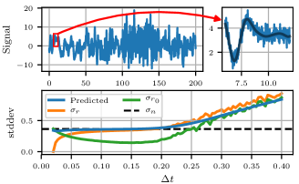
Figure 2: Top: 50Hz test signal and noise (right subplot is a detail). Bottom: standard deviations as functions of knot spacing. $\sigma_{r}$ is the empirical residual standard deviation, $\sigma_{n}$ is the noise standard deviation, which is used in [21] to predict $\sigma_{r}$, Predicted is the proposed residual noise prediction. $\sigma_{r_{0}}$ is the residual with respect to the noise-free signal $x_{0}(t)$.

2.2 A simple 1D illustration

In figure 2 we illustrate a simple experiment that demonstrates the behaviour of our proposed residual error prediction (9). In figure 2 top left, we show a test signal, $x(t)$, which is the sum of a true signal, $x_{0}(t)$, and white Gaussian noise $n(t)$ with variance $\sigma_{n}^{2}$. The true signal has been generated by filtering white noise to produce a range of different frequencies and amplitudes. In figure 2 top right, we show a detail of the signal, where the added noise is visible.

We now apply a least-squares spline fit to the signal $x(t)$, to obtain the spline $\hat{x}(t)$, with control points $\boldsymbol{\Theta}=(\theta_{1},\ldots,\theta_{K})^{T}$ and basis functions $B(t)$:

$$\hat{x}(t|\boldsymbol{\Theta})=\sum_{k=1}^{K}\theta_{k}B(t-k\Delta t)\,.$$ (12)

This is repeated for a range of knot spacings, $\Delta t$, each resulting in a different residual $r(t)=x(t)-\hat{x}(t)$. The residual standard deviation $\sigma_{r}$ is plotted in figure 2, bottom. We make the same plot for the residual $r_{0}(t)=x_{0}(t)-\hat{x}(t)$ which measures the error compared to the true signal. The resulting $\sigma_{r_{0}}$ curve has a minimum at approximately $\Delta t=0.15$, which is thus the optimal knot spacing. The fact that the actual residual $\sigma_{r}$ decreases for knot spacings below this value thus indicates overfitting. From the experiment, we can also see that the implicit assumption made in [21] that the noise standard deviation $\sigma_{n}$ can predict $\sigma_{r}$ is reasonable for knot spacings at or below the optimal value. However, for larger knot spacings (at the right side of the plot) this assumption becomes increasingly inaccurate.

2.3 Selecting the knot spacing

Instead of deciding on a knot spacing explicitly, a more convenient design criterion is the amount of approximation error introduced by the spline fit. To select a suitable knot spacing, $\Delta t$, we thus first decide on a quality value, $\hat{q}\in(0,1]$, that corresponds to the fraction of signal energy we want the approximation to retain. For a given signal, $x(t)$, with the DFT, ${\bf X}$, we define the quality value as the ratio between the energy, before and after spline fitting:

$$q(\Delta t)=\frac{\mathbb{E}\{{\bf H}(\Delta t)\cdot{\bf X}\}}{\mathbb{E}\{{\bf X}\}}$$ (13)

Here ${\bf H}(\Delta t)$ is the scaled frequency response of the spline approximation, see section 2.1. By constraining $H(f)$ to preserve the DC-component after a change of variables, i.e., $H(0)=1$, the change of variables simplifies to a scaling of the original frequency response, $H(f,\Delta t)=H(\Delta tf)$ .

To find a suitable knot spacing for the signal, we search for the largest knot spacing $\Delta t$ for which $q(\Delta t)\geq\hat{q}$. We do this by starting at the maximum allowed knot spacing, and then decrease $\Delta t$ until $q(\Delta t)\geq\hat{q}$. At this point we use the bounded root search method by Brent [6] to find the exact point, $\Delta t$, where $q(\Delta t)=\hat{q}$.

3 Visual-inertial fusion

We will use the residual error prediction introduced in section 2 to balance visual-inertial fusion on rolling shutter cameras. Our formulation is largely the same as in the SplineFusion method [21]. In addition to the improved balancing, we modify the SplineFusion method, as follows: (1) we interpolate in $\mathbb{SO}(3)\text{ and }\mathbb{R}^{3}$ instead of in $\mathbb{SE}(3)$, (2) we use a rolling shutter reprojection method based on observation time instead of performing Newton-optimization, and (3) we add a robust error norm for image residuals.

Given IMU measurements $\{\boldsymbol{\omega}_{n}\}_{1}^{N},\{{\bf a}_{l}\}_{1}^{L}$, and tracked image points, the objective is to estimate the trajectory ${\bf T}(t)$, and the 3D landmarks that best explain the data. This is done by minimizing a cost function $J(\boldsymbol{\theta},\boldsymbol{\rho})$ where $\boldsymbol{\theta}$ and $\boldsymbol{\rho}$ are trajectory and landmark parameters, respectively. We parameterize landmarks using the inverse depth relative to a reference observation, while the trajectory parameters are simply the spline control points for the cubic B-splines. We define our cost function as

$$J(\boldsymbol{\theta},\boldsymbol{\rho})= \sum_{k,m}\phi({\bf x}_{k,m}-\pi({\bf x}_{k,0},{\bf T}(t_{k,m}){\bf T}(t_{k,0})^{-1},\rho_{k}))$$

$$+ \sum_{n}||\boldsymbol{\omega}_{n}-\nabla_{\omega}{\bf T}(t_{n})||^{2}_{{\bf W}_{g}}$$ (14)

$$+ \sum_{l}||{\bf a}_{l}-\nabla^{2}_{a}{\bf T}(t_{l})||^{2}_{{\bf W}_{a}}\,.$$

Here, $\phi$ is a robust error norm. Each landmark observation ${\bf x}_{k,m}$ belongs to a track $\left\{{\bf x}_{k,m}\right\}_{m=0}^{M}$, and has an associated inverse depth $\rho_{k}$. The function $\pi(\cdot)$ reprojects the first landmark observation into subsequent frames using the trajectory and the inverse depth. The norm weight matrices ${\bf W}_{g}$ and ${\bf W}_{a}$ are in general matrices, but in our experiments they are assumed to be isotropic, which results in

$${\bf W}_{g}={\bf I}\frac{1}{\hat{\sigma}_{r,g}^{2}}\,,\text{ and }{\bf W}_{a}={\bf I}\frac{1}{\hat{\sigma}_{r,a}^{2}}\,,$$ (15)

where $\hat{\sigma}_{r,g}^{2}$ and $\hat{\sigma}_{r,a}^{2}$ are the predicted residual variances for the two modalities, see (11).

The operators $\nabla_{\omega}$ and $\nabla^{2}_{a}$ in (14) represent inertial sensor models which predict gyroscope and accelerometer readings given the trajectory model ${\bf T}(t)$, using analytic differentiation. The inertial sensor models should account for at least biases in the accelerometer and gyroscope, but could also involve e.g. axis misalignment.

The robust error norm $\phi$ is required for the image residuals since we expect the image measurements to contain outliers that, unless handled, will result in a biased result. We use the Huber error norm with a cut-off parameter $c=2$. The gyroscope and accelerometer measurements do not contain outliers, and thus no robust error norm is required here.

3.1 Quality measurement domains

In order to apply the method in section 2 on a spline defining a camera trajectory, we need to generalize estimation to vector-valued signals, and also to apply it in measurement domains that correspond to derivatives of the sought trajectory.

The gyroscope senses angular velocity, which is the derivative of the $\mathbb{SO}(3)$ part of the sought trajectory. From the derivative theorem of B-splines [25], we know that the derivative of a spline is a spline of degree one less, with knots shifted by half the knot spacing. Thus, as the knot spacing in the derivative domain is the same, we can impose a quality value $\hat{q}_{\text{g}}$ on the gyro signal to obtain a knot spacing $\Delta t_{\text{g}}$ for the $\mathbb{SO}(3)$ spline.

In order to apply (13) to the gyroscope signal, $\boldsymbol{\omega}(t)$, we need to convert it to a 1D spectrum $X_{g}(f)$. This is done by first applying the DFT along the temporal axis. We then compute a single scalar for each frequency component using the scaled $L_{2}$-norm:

$$X_{g}(f)=\sqrt{\frac{1}{3}}\|\boldsymbol{\Omega}(f)\|\,\;\text{where}\;\;\boldsymbol{\Omega}(f)=\begin{bmatrix}\Omega_{x}(f)\\ \Omega_{y}(f)\\ \Omega_{z}(f)\end{bmatrix}\,.$$ (16)

We also set $X_{g}(0)=0$ to avoid that a large DC component dominates (13). Conceptually this also makes sense as a spline depends only on the shape of the measurements, and not the choice of origin.

To find a knot spacing for the $\mathbb{R}^{3}$-spline, the connection is not as straightforward as for the $\mathbb{SO}(3)$ part of the trajectory. Here we employ the IMU data from the accelerometer, and use the same formulation as in (16) to compute a 1D spectrum $X_{a}(f)$, again with zero DC, $X_{a}(0)=0$.

In contrast to the gyroscope, however, the accelerometer measurements are induced by changes in both $\mathbb{R}^{3}$ and $\mathbb{SO}(3)$: the linear acceleration, and the current orientation of the gravity vector. Because of the gravitational part, the measurements are always in the order of $1g$, the standard gravity, which is very large compared to most linear accelerations. For a camera with small rotation in pitch and roll, most of the gravity component will end up in the DC component, and thus not influence the result. For large rotations, however, the accelerometer will have an energy distribution that is different from the position sequence of the final spline.

In the experiment section, we evaluate the effectiveness of the quality estimates for both gyroscope and accelerometer.

4 Experiments

Our experiments are mainly designed to verify the spline error weighting method (SEW), presented in sections 2 and 3. However, they also hint at some of the benefits of incorporating inertial measurements in SfM: metric scale, handling of visual dropout, and reduced need for initialization. The experiments are all based on real data, complementing the synthetic example already presented in section 2.2.

4.1 Datasets

We recorded datasets for two use-cases: Bodycam and Handheld. All sets were recorded outdoors using a GoPro Hero 3+ Black camera with the video mode set to 1080p at 30Hz. For the bodycam datasets the camera was strapped securely to the wearer’s chest using a harness, pointing straight forward. For the handheld datasets, the camera motion was less constrained but was mostly pointed forwards and slightly sideways.

To log IMU data we used a custom-made IMU logger based on the InvenSense MPU-9250 9-axis IMU. Data was captured at 1000 Hz, but was downsampled to 300 Hz for the experiments.

The camera was calibrated using the FOV model in [7]. An initial estimate of the time offset between the camera and IMU, as well as their relative orientation, was found using the software package Crisp [20]. Since Crisp does not handle accelerometer biases we refined the calibration using the same spline-based SfM pipeline as used in the experiments. Calibration was refined on a short time interval with IMU biases, time offset, and relative orientation as additional parameters to estimate.

When recording each dataset, we used a tripod with an indicator bar to ensure that each dataset ended with the camera returned to its starting position ($\pm 2$ cm). This enables us to use endpoint error (EPE) as a metric in the experiments, $\text{EPE}=\|{\bf p}(t_{0})-{\bf p}(t_{\text{end}})\|$, where ${\bf p}(t)$ is the positional spline. To gauge the scale error after reconstruction, we measured a few distances in each scene using a measuring tape.

Example frames and final reconstructions of the datasets can be seen in figures 1, 3, 4, and 5. To improve visualization the example figures have been densified by triangulating additional landmarks using the estimated trajectory.

Figure 3: Render of model estimated on Bodycam 1 dataset. Top: model rendered using Meshlab. Bottom: Sample frames from dataset.

Figure 4: Render of model estimated on Bodycam 2 dataset. Top: model rendered using Meshlab. Bottom: Sample frames from dataset.

4.2 Structure from motion pipeline

To not distract from the presented theory, we opted for a very simple structure from motion pipeline that can serve as a baseline to build on.

We generate visual observations by detecting FAST keypoints [22] with a regular spatial distribution enforced using ANMS [11]. These are then tracked in subsequent frames using the OpenCV KLT-tracker [5]. For added robustness, we performed backtracking and discarded tracks which did not return to within $0.5$ pixels of its starting point. Using tracking instead of feature matching means that landmarks that are detected more than once will be tracked multiple times by the system. In addition, the visual data does not contain any explicit loop closures, which in turn means that correct weighting of the IMU residuals become more important to successfully reconstruct the trajectory.

The trajectory splines are initialized with their respective chosen knot spacing, such that they cover all frames in the data. The spline control points are initialized to $\mathbf{0}\in\mathbb{R}^{3}$ and ${\bf I}\in\mathbb{SO}(3)$ respectively. All landmarks are placed at infinity, with inverse depths $\rho=0$. Note that we are not using any initialization scheme like essential matrix estimation and triangulation to give the system a reasonable starting point.

The pipeline consists of four phases:

Initial

Rough reconstruction using keyframes.

Cleanup ($\times 2$)

Reoptimize using only landmarks with a mean reprojection error below a threshold.

Final

Optimize over all frames.

We now describe the phases in more detail. To start the reconstruction we first select a set of keyframes. Starting with the first frame we insert a new keyframe whenever the number of tracked landmarks from the previous keyframe drops below $75\%$. To avoid generating too many keyframes we add the constraint that the distance between two keyframes must be at least 6 frames.

The starting set of observations are then chosen from the keyframes using ANMS [11], weighted by track lengths, such that each keyframe provides at most $n=100$ observations. After the initial phase is completed, we do two cleanup phases. During a cleanup phase we first determine the mean reprojection error for all landmarks that are visible in the keyframes. We then pick a new set of observations (at most $n$ per frame) from landmarks with mean reprojection errors below a threshold. These thresholds are set to $8$ and $5$ pixels, respectively.

For the final phase we select the landmarks with a mean reprojection error below $3$ pixels, and add observations for all frames.

Figure 5: Render of model estimated on Handheld 2 dataset. Top: model rendered using Meshlab. Bottom: Sample frames from dataset.

4.3 Prediction of quality

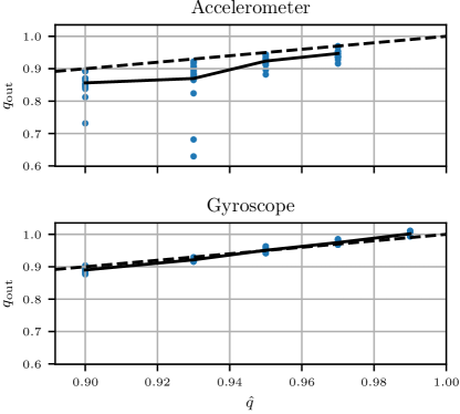
Figure 6: Actual quality ($q_{\text{out}}$) as a function of requested quality ($\hat{q}$) for both accelerometer and gyroscope. The blue markers are the individual data points, and the solid line their mean. The dashed line shows the ideal $q_{\text{out}}=\hat{q}$.

We now test how well the requested quality $\hat{q}$ corresponds to the obtained quality after spline fit. For each dataset we performed reconstructions with a range of different quality values for the accelerometer and gyroscope. The requested quality value then determines the knot spacing, and IMU weights used by the optimizer according to the theory presented in sections 2 and 3. All reconstructions for a dataset were initialized with the same set of keyframes and initial observations.

As we can see in figure 6 the obtained quality for the gyroscope corresponds well with the requested value. For the accelerometer however, the obtained quality is consistently slightly lower. The outliers in the accelerometer plot correspond to the lowest gyroscope quality values. Since the accelerometer measurements depend also on the orientation estimate, it is expected that a reduction in gyroscope quality would influence the accelerometer quality as well, see section 3.1.

4.4 Importance of correct weighting

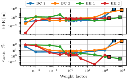
Figure 7: Endpoint error and scale error as functions of the IMU residual weights. The weight factor was multiplied with the base weights found using (15). The dashed line shows the weights selected by SEW. Measurements surrounded by a box represent the weighting used in SplineFusion. BC: Bodycam, HH: Handheld.

To investigate how well our method sets the IMU residual weights, we made several reconstructions using the same knot spacing but different weights. The knot spacing and base weights for the IMU residuals were first selected using the theory described in sections 2 and 3. We then performed multiple reconstructions with the IMU weights scaled by a common factor. All reconstructions for a given dataset used the same initial set of keyframes and observations. In figure 7 we plot the endpoint error and scale error as functions of this factor. The scale error is defined as $e_{\text{scale}}=|l_{\text{true}}-\hat{l}|/l_{\text{true}}$, where $l_{\text{true}}$ is the true length as measured in the real world, and $\hat{l}$ is a length that is triangulated, from manually selected points, using the reconstructed trajectory.

Figure 7 shows that SEW produces weights which are in the optimal band where both errors are low. In contrast, the inverse noise covariance weights used by SplineFusion (the right-most data points) are consistently a bad choice.

4.5 Visual dropout

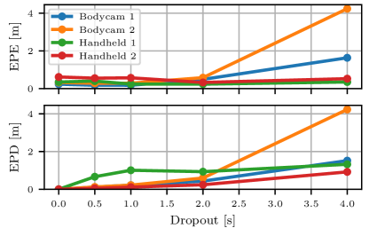
Figure 8: Endpoint error and endpoint distortion as functions of dropout time. The dropout is the number of seconds for which no visual observations were available.

One of the benefits of including IMU data in structure from motion is that we can handle short intervals of missing visual observations. These could be due to changes in lighting, or because the observed scenery has no visual features (white wall, clear sky, etc.).

To investigate visual dropout in a controlled manner we simulate dropouts by removing the last $n$ frames in each dataset. The trajectory estimate in this part will then depend on IMU measurements only. In figure 8 we show the endpoint error and endpoint distortion (EPD) for different lengths of dropout. The endpoint distortion is the distance from the estimated endpoint under dropout to the endpoint without dropout. It thus directly measures the drift caused by the dropout.

As expected the errors increase with the dropout time, but are quite small for dropout times below a second. The dropout error is sensitive to the IMU/camera calibration, and especially to correct modeling of the IMU biases. Given that these are accurately estimated, the IMU provides excellent support in case of brief visual dropout.

4.6 Comparison to SplineFusion

Finally we make an explicit comparison with SplineFusion as described in [21], but with the three modifications stated in section 3. The only difference between SEW and SplineFusion in the following comparison is with regards to knot spacing and IMU residual weights: For SplineFusion we set both spline knot spacings to $\Delta t=0.1$ seconds, and IMU residual weights to the inverse of the measurement noise covariances, as was done in [21]. For SEW (the proposed method) the knot spacings and residual weights were chosen using quality values $q_{\text{acc}}=0.97$ and $q_{\text{gyro}}=0.99$. This resulted in knot spacings averaging around $0.04$ seconds.

In figure 9 we show the reconstructed trajectories projected onto the XY-plane, and table 1 shows the corresponding endpoint and scale errors. A perfect reconstruction should have the trajectories start and end at exactly the same point, with zero endpoint error. It is clear that the SplineFusion settings work reasonably well in the handheld case, but completely fails for bodycams. However, even in one of the handheld sequences the scale error for SplineFusion is a magnitude larger than that of SEW. It is unsurprising that the SplineFusion settings work on the Handheld 2 dataset, as the motions in this dataset are relatively smooth compared to the others.

In figure 10 we plot the residual distributions after convergence on the Handheld 2 dataset. Ideally the IMU residuals should be normally distributed with mean $\mu=0$ and standard deviation $\sigma=1$. The image residuals could contain outliers, and are also mapped through the robust error norm $\phi$, and are thus not necessarily normally distributed. It is clear that SEW produces residuals which are close to standardized, while the inverse noise covariance weighting of SplineFusion does not.

	EPE [m]		$e_{\text{scale}}$ [%]
	SEW	SplineFusion	SEW	SplineFusion
Bodycam 1	0.22	37.95	3.4%	124.2%
Bodycam 2	0.40	27.86	8.7%	423.1%
Handheld 1	0.30	0.52	1.4%	19.0%
Handheld 2	0.56	0.94	2.0%	1.7%

Table 1: Comparison of SEW and SplineFusion

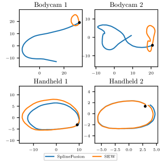
Figure 9: Comparison of obtained trajectories for SplineFusion and SEW. Trajectories have been aligned to share the starting point (black dot). All trajectories should ideally start and end at the same point.

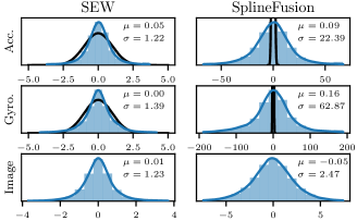
Figure 10: Blue: Residual distribution after convergence for the Handheld 2 dataset. Black: PDF of the standard normal distribution $\mathcal{N}(0,1)$ that is expected for the IMU residuals.

5 Conclusions and future work

We have introduced a method that balances residuals from different modalities. In the experiments we applied the method to continuous-time structure from motion, using measurements from KLT-tracking and an IMU. This simple setup was used to highlight the advantages with the proposed error weighting scheme. In order to further improve the robustness in this particular application, one could incorporate, by now classical ideas from SfM, such as invariant features, and loop-closure detection.

The proposed spline error weighting uses empirical spectra in the different measurement modalities. Such spectra are however often characteristic of specific types of motion, e.g. handheld and bodycam sequences have characteristic within group spectra, and these could be learned and applied directly to new sequences of the same type. Such learned characteristic spectra could be useful as a priori information when adapting spline error weighting to do on-line visual-inertial fusion.

Another potential improvement is to derive a better residual error prediction for the accelerometer, that properly accounts for the interaction with the sensor orientation changes. The quality experiment in figure 6 revealed a consistent underestimation of the approximation quality, and a better prediction should remedy this.

We plan to release our spline error weighting framework for visual-inertial fusion under an open source license.
Acknowledgements: This work was funded by the Swedish Research Council through projects LCMM (2014-5928) and and EMC2 (2014-6227). The authors also thank Andreas Robinson for IMU logger hardware design.

References

- [1] S. Anderson and T. D. Barfoot. Full STEAM ahead: Exactly sparse gaussian process regression for batch continuous-time trajectory estimation on SE(3). In IEEE International Conference on Intelligent Robots and Systems (IROS15), 2015.
- [2] S. Anderson, F. Dellaert, and T. D. Barfoot. A hierarchical wavelet decomposition for continuous-time SLAM. In IEEE International Conference on Robotics and Automation (ICRA14), 2014.
- [3] S. Anderson, K. MacTavish, and T. D. Barfoot. Relative continuous-time slam. The International Journal of Robotics Research, 34(12):1453–1479, 2015.
- [4] T. Bailey and H. Durrant-Whyte. Simultaneous localization and mapping (SLAM): part II. IEEE Robotics & Automation Magazine, 13(3):108–117, sep 2006.
- [5] J.-Y. Bouguet. Pyramidal implementation of the lucas kanade feature tracker. Intel Corporation, Microprocessor Research Labs, 2000.
- [6] R. P. Brent. Algorithms for Minimization without Derivatives, chapter Chapter 4: An Algorithm with Guaranteed Convergence for Finding a Zero of a Function. Englewood Cliffs, NJ: Prentice-Hall, 1973.
- [7] F. Devernay and O. Faugeras. Straight lines have to be straight: Automatic calibration and removal of distortion from scenes of structured environments. Machine Vision and Applications, 13(1):14–24, 2001.
- [8] C. Forster, L. Carlone, F. Dellaert, and D. Scaramuzza. IMU preintegration on manifold for efficient visual-inertial maximum-a-posteriori estimation. In Robotics: Science and Systems (RSS’15), Rome, Italy, July 2015.
- [9] P. Furgale, T. D. Barfoot, and G. Sibley. Continuous-time batch estimation using temporal basis functions. In IEEE International Conference on Robotics and Automation (ICRA12), 2012.
- [10] P. Furgale, C. H. Tong, T. D. Barfoot, and G. Sibley. Continuous-time batch trajectory estimation using temporal basis functions. International Journal of Robotics Research, 2015.
- [11] S. Gauglitz, L. Foschini, M. Turk, and T. Hollerer. Efficiently selecting spatially distributed keypoints for visual tracking. In 18th IEEE International Conference on Image Processing, 2011.
- [12] G. Hanning, N. Forslöw, P.-E. Forssén, E. Ringaby, D. Törnqvist, and J. Callmer. Stabilizing cell phone video using inertial measurement sensors. In The Second IEEE International Workshop on Mobile Vision, 2011.
- [13] J. Hedborg, P.-E. Forssén, M. Felsberg, and E. Ringaby. Rolling shutter bundle adjustment. In IEEE Conference on Computer Vision and Pattern Recognition, June 2012.
- [14] C. Jia and B. L. Evans. Online calibration and synchronization of cellphone camera and gyroscope. In IEEE Global Conference on Signal and Information Processing (GlobalSIP), December 2013.
- [15] J. Kopf, M. F. Cohen, and R. Szeliski. First-person hyper-lapse videos. In SIGGRAPH Conference Proceedings, 2014.
- [16] M. Li, B. H. Kim, and A. I. Mourikis. Real-time motion tracking on a cellphone using inertial sensing and a rolling-shutter camera. In IEEE International Conference on Robotics and Automation ICRA’13, 2013.
- [17] S. Lovegrove, A. Patron-Perez, and G. Sibley. Spline fusion: A continuous-time representation for visual-inertial fusion with application to rolling shutter cameras. In British Machine Vision Conference (BMVC). BMVA, September 2013.
- [18] Z. Mihajlovic, A. Goluban, and M. Zagar. Frequency Domain Analysis of B-Spline Interpolation. ISIE’99 - Bled, Slovenia, pages 193–198, 1999.
- [19] L. Oth, P. Furgale, L. Kneip, and R. Siegwart. Rolling shutter camera calibration. In IEEE Conference on Computer Vision and Pattern Recognition (CVPR13), pages 1360–1367, Portland, Oregon, June 2013.
- [20] H. Ovrén and P.-E. Forssén. Gyroscope-based video stabilisation with auto-calibration. In IEEE International Conference on Robotics and Automation ICRA’15, 2015.
- [21] A. Patron-Perez, S. Lovegrove, and G. Sibley. A spline-based trajectory representation for sensor fusion and rolling shutter cameras. International Journal on Computer Vision, 113(3):208–219, 2015.
- [22] E. Rosten, R. Porter, and T. Drummond. Faster and better: A machine learning approach to corner detection. IEEE Trans. Pattern Anal. Mach. Intell., 32(1), Jan. 2010.
- [23] G. Sibley, C. Mei, and I. Reid. Adaptive relative bundle adjustment. In Robotics: Science and Systems (RSS’09), 2009.
- [24] B. Triggs, P. Mclauchlan, R. Hartley, and A. Fitzgibbon. Bundle adjustment – a modern synthesis. In Vision Algorithms: Theory and Practice, LNCS, pages 298–375. Springer Verlag, 2000.
- [25] M. Unser. Splines – a perfect fit for signal and image processing. IEEE Signal Processing Magazine, 16(6):22–38, 1999.
- [26] M. Unser, A. Aldroubi, and M. Eden. B-spline signal processing. II. Efficiency design and applications. IEEE Transactions on Signal Processing, 41(2):834–848, 1993.