Adversarial Clustering: A Grid Based Clustering Algorithm Against Active Adversaries

Wutao Wei, Bowei Xi, Murat Kantarcioglu

Purdue University, Purdue University, University of Texas, Dallas

Corresponding to:

Bowei Xi, Department of Statistics, Purdue University,

West Lafayette, IN, 47907. xbw@purdue.edu

Abstract: Nowadays more and more data are gathered for detecting and preventing cyber attacks. In cyber security applications, data analytics techniques have to deal with active adversaries that try to deceive the data analytics models and avoid being detected. The existence of such adversarial behavior motivates the development of robust and resilient adversarial learning techniques for various tasks. Most of the previous work focused on adversarial classification techniques, which assumed the existence of a reasonably large amount of carefully labeled data instances. However, in practice, labeling the data instances often requires costly and time-consuming human expertise and becomes a significant bottleneck. Meanwhile, a large number of unlabeled instances can also be used to understand the adversaries’ behavior. To address the above mentioned challenges, in this paper, we develop a novel grid based adversarial clustering algorithm. Our adversarial clustering algorithm is able to identify the core normal regions, and to draw defensive walls around the centers of the normal objects utilizing game theoretic ideas. Our algorithm also identifies sub-clusters of attack objects, the overlapping areas within clusters, and outliers which may be potential anomalies.

Keyword: Adversarial Clustering, Adversarial Machine Learning, Cyber Security, Big Data, Game Theory

1 Introduction

Increasingly data analytics techniques are being applied to large volumes of system monitoring data to detect cyber security incidents. The ultimate goal is to provide cyber security analysts with robust and effective insights derived from big data. Unlike most other application domains, cyber security applications often face adversaries who actively modify their strategies to launch new and unexpected attacks. The existence of such adversaries results in cyber security data that have unique properties. Firstly, the attack instances are frequently being modified to avoid detection. Hence a future dataset no longer shares the same properties as the current training dataset. Secondly, when a previously unknown attack happens, security analysts need to respond to the new attack quickly without the help of readily labeled instances in their database to assist their work. Thirdly, adversaries can be well funded and make big investments to camouflage the attack instances. Therefore despite significant effort invested by the domain experts, a vast majority of the instances in their database may remain unlabeled. For example, a new malware can incorporate large amounts of legitimate code to masquerade as legitimate software and obfuscate its binary. In other cases, it may become laborious and expensive to label an instance.

Thus data analytics techniques for cyber security must also have unique capabilities. They need to be resilient against the adaptive behavior of the adversaries, and are able to quickly detect previously unknown and unlabeled new attack instances. Hence, recently, various adversarial machine learning techniques have been developed to counter adversarial adaptive behaviors. However those previous adversarial machine learning work is mostly under the main assumption of the availability of large amounts of labeled instances (i.e., normal versus malicious objects). Although large amounts of data are generated by the cyber security applications, we often have few properly labeled instances to construct an effective classifier.

Given a large amount of unlabeled data, defender needs to capture the adversarial behavior, identify suspicious instances as anomalies for a more detailed investigation, and quickly respond to new attacks. However clusters identified by traditional clustering algorithms are likely mixed, since with a few attack objects, adversaries can bridge the gap between two previously well separated clusters. Sometimes a handful of labeled attack and normal instances are available. There are too few of them to build a classifier, yet they offer valuable information about the adversaries. In this paper, we develop a novel adversarial clustering algorithm so that we need only a few labeled instances to build robust defensive algorithm against the attack objects. Our algorithm can identify the centers of normal objects, sub-clusters of attack objects, and the overlapping areas where adversaries have successfully placed the attack objects. We then draw defensive walls around the centers of the normal objects utilizing game theoretic ideas. Our algorithm also identifies outliers as potential anomalies and outlying unknown clusters for further investigation.

Semi-supervised learning techniques also utilize information from both labeled and unlabeled instances. Adversarial clustering and semi-supervised learning operate under very different assumptions. In adversarial settings, attackers purposely modify the attack objects to make them similar to normal objects, though suffering a cost for doing so. Hence the assumptions commonly used for semi supervised learning do not hold for adversarial clustering. Instead we observe that objects similar to each other belong to different classes, while objects in different clusters belong to the same class. In adversarial settings, within each cluster, objects from two classes can overlap significantly. Consequently, adversarial clustering and semi-supervised learning techniques have very different goals too. Semi-supervised learning aims to assign labels to all the unlabeled objects with the best accuracy. Our adversarial clustering algorithm aims to identify the overlapping regions, and the core areas of the normal objects, within each cluster. The overlapping regions and outliers are not labeled by our algorithm. We draw defensive walls around the centers of the normal objects. The shape and the size of the defensive walls are determined through a game theoretic study. Inside the defensive walls, we have nearly pure normal objects, despite an increased error of blocking out the normal objects mixed with the attack objects outside of the walls. Adversarial clustering draws an analogy to airport security. A small number of passengers use the fast pre-check lane at the security checkpoint, analogous to the normal objects inside the defensive walls. All other passengers must go through more time consuming security check, analogous to the objects outside the walls. The goal is not to let a single terrorist enter an airport, at a cost of blocking out many normal objects. Meanwhile the ability to identify the overlapping regions leads to a more focused security check procedure, where attack and normal objects are similar to each other. We compare our algorithm with semi-supervised learning algorithms in Section 4.

The paper is organized as follows. Section 1.1 discusses the related work. In Section 2, we present our adversarial clustering algorithm. In Section 3, we conduct a game theoretic study to examine the sizes and the shapes of different defensive walls used in our adversarial clustering algorithm. In Section 4, we evaluate our algorithm with simulated and a network intrusion data sets. Section 5 concludes the paper.

1.1 Related Work

Robust learning techniques have been proposed in the past, for example, to defeat poisoning attacks [35], purposely generated malicious errors [24], and missing or corrupted features [15]. Classification in adversarial settings has also received considerable attention in the literature, e.g., [14, 20, 28, 29, 47]. In [9, 21], Stackelberg game is used to model the sequential actions between a defender/classifier and active adversaries. Adversarial classification techniques were developed for the Facebook social network to defeat the fake and spam accounts [40]. However even with the information obtained from a large training sample of labeled normal and attack objects, building a robust classifier to block out the attack objects, which are constantly being modified by adversaries to avoid detection, is not an easy task.

Compared with adversarial classification, there is fewer work on adversarial clustering, which is a much harder learning problem. [4] considered the problem of evaluating the security of clustering algorithms in an adversarial setting. [4] then evaluated the security of single linkage hierarchical clustering algorithm under poisoning attacks and obfuscation attacks. [5] further studied the effects of poisoning attacks on complete linkage hierarchical clustering algorithm. [16] showed that a few well-constructed attack objects could lead to a larger mixed cluster, and hence significantly reduce the effectiveness of a clustering algorithm. [41] showed that subspace clustering has a certain tolerance for noisy or corrupted data.

Semi-supervised learning techniques utilizes information from both labeled and unlabeled instances. It has an extensive literature. In general there are two types of semi-supervised learning techniques, semi-supervised classification and semi-supervised clustering. There are many different approaches for semi-supervised classification, such as transductive support vector machine (TSVM), generative mixture models, self-training and co-training. TSVM extends SVM to the semi-supervised learning scenario. Labels are assigned to the unlabeled instances such that the classification boundary has the maximum margin on the original labels and newly assigned labels (e.g., [10, 45, 38]). TSVM avoids the high density regions, which may not be the optimal solution when two classes are heavily overlapped. Under mixture model assumption, EM algorithm is used for semi-supervised classification (e.g., [32, 18]). This approach allows the classification boundary to go through the densest region of the data points. However users need to pay attention to model identifiability issue and whether the model assumption fits the data or not (e.g., [31, 33, 12]). Self-training approach iteratively assigns labels to new data points, and then includes both the existing labels and newly assigned labels to train another classifier (e.g., [34, 13, 19]). Co-training splits the available features into two sets and build two classifiers, each using only one set of features. In an iterative process, each classifier learns from the other one with the most confident predicted labels (e.g., [3, 11, 46]).

Often semi-supervised clustering algorithms use pairwise must-link and cannot-link constraints. Must-links ensure the objects with identical labels are grouped in the same cluster, while cannot-links ensure the objects with different labels are in different clusters (e.g. [2, 6, 22]). Meanwhile many work extends K-means algorithm to semi-supervised clustering settings (e.g., [42, 7, 43]). [8] developed a hierarchical density based semi-supervised clustering algorithm. However if the density varies significantly among clusters, the algorithm has difficulty to extract the natural cluster structure. [26] extends DBSCAN to semi-supervised settings. Instead of having one set of values for the parameters as in DBSCAN, [26] finds multiple sets of parameter values to better handle the situation when densities vary significantly among clusters.

Our adversarial clustering algorithm has a very different goal. Compared with semi-supervise learning, we do not label all the previously unlabeled objects and attempt to achieve the maximum accuracy. Instead we identify the centers of normal objects using defensive walls. We focus on having nearly pure normal objects inside the walls, often at the expense of blocking out many normal objects mixed with abnormal objects. Hence the overall accuracy of our algorithm may decrease but we identify the center normal regions where the percentage of normal objects is much higher, and can be considered as relatively safe regions. We do not label the objects in the regions where normal and abnormal objects are mixed. Instead we mark out the whole mixed areas, where attacks take place and objects must be examined carefully. We also leave unknown clusters and outliers unlabeled, since they should be investigated carefully as being potential anomalies or a new attack.

2 Adversarial Clustering

In cyber security applications, adversaries actively manipulate the objects under their control to break through a defensive algorithm. Hence the properties of the data under attack are drastically different from the data without an attack. Even though the normal population remains unchanged, the adversaries can inject a small amount of attack objects to fill in the gap between abnormal clusters and normal clusters, and make previously relatively pure normal clusters mixed, as pointed out in [4, 5, 16]. Traditional clustering algorithms are able to produce clusters and a few outliers. Without any labeled instances, that is the only result we can expect, not knowing whether a cluster is mixed, or nearly purely normal or abnormal. On the other hand, if a large number of labeled instances are available, we can build a classifier with a well defined classification boundary that separates the normal and abnormal objects within one cluster, and separate the relative pure normal clusters from the abnormal objects.

In this paper, we consider a scenario where there are a large number of unlabeled instances and only a handful of labeled instances (i.e., the number labeled being far less than the number of unlabeled ones). A classifier created using very few labeled objects is very inaccurate when being applied to the large number of unlabeled ones. On the other hand clusters, produced by traditional clustering algorithms, may become mixed clusters under attack, where extra efforts are needed to identify normal and abnormal regions inside these mixed clusters. Therefore we develop a grid based adversarial clustering algorithm, which is able to utilize the handful of labeled objects, identify relatively pure normal and abnormal regions within one cluster and their overlapping area, and further identify outliers and outlying clusters which need more effort to investigate their properties.

A classifier with a well defined classification boundary is analogous to a point estimate. When the sample size is too small (i.e., too few labeled instances), a point estimate is way too inaccurate. Hence our clustering algorithm identify overlapping areas between the normal regions and the abnormal regions, analogous to confidence regions. When a large number of labeled instances are available, a classification boundary is a defensive wall against the adversaries, since it blocks out the attack objects. When facing active adversaries, a classifier needs to be more conservative, i.e., a classification boundary is pulled back toward the center of the normal population, as shown in [47]. With a large number of unlabeled instances, our adversarial clustering algorithm offers more valuable information to capture both normal and abnormal regions. Our adversarial clustering algorithm then plays a conservative strategy. We draw defensive walls inside the normal regions to protect the relatively pure normal centers. All objects outside of the walls need to be examined carefully, while many normal objects can be blocked out. How conservative the defensive walls need to be is determined through a game theoretic study in Section 3. If the defensive walls are too close to the center of the normal regions, we miss a large portion of the relatively pure normal areas. If the defensive walls are too relaxed, we have too many attack objects in the walls. Hence we utilize the equilibrium information to determine the sizes of the conservative defensive walls for our algorithm.

2.1 A Grid Based Defensive Clustering Algorithm

Since cyber security applications often produce big data sets, we need a computationally efficient algorithm, which needs to be easy to tune as well. Inspired by a traditional grid based clustering algorithm [44], we develop a grid based adversarial clustering algorithm (ADClust). Our algorithm applies a Gaussian kernel classifier to compute the probability scores for every unlabeled data points. Then using a pre-specified weight ,we obtain re-weighted density of the data points. In the first pass, our algorithm groups the data points into normal sub-clusters, abnormal sub-clusters, unlabeled sub-clusters and unlabeled outliers. Notice that the choice of the weight affects the size of the overlapping areas and the normal and abnormal regions. Then in a second pass, we do not use label information, and simply group the data points into large unlabeled clusters and identify unlabeled outliers. The next step is to match the normal, abnormal, unlabeled smaller clusters from the first pass with the unlabeled larger clusters from the second pass. This way we are able to identify normal and abnormal regions within one cluster along with the unlabeled overlapping regions. The last step is to play a conservative strategy, drawing defensive walls inside normal regions to ensure that we identify relatively pure normal core positions. Figures 8, 9, and 10 in Section 4 show how our algorithm work on three simulated datasets.

During the initialization stage of our algorithm we create the cells, compute the distance threshold RT and the density threshold DT. We choose a pre-determined positive weight $k$ to assign re-weighted density to every unlabeled point. The value of $k$ affects the size of the overlapping regions. Section 4 examine different $k$ values and recommend $k$ around 30. $coefRT$ and $coefDT$ are also tuning parameters. In Section 4, we set $coefRT=20$ and $coefDT=0.95$, which achieve good results. There are three initialization steps.

Initialization Step 1. Creating cells: For every variable $X_{i}$, divide its range [min$(X_{i})$, max$(X_{i})$] into $m_{i}$ equal sized sections, $i=1,...,q$. We choose the number $m_{i}$ to ensure each section has roughly $5\%$ to $10\%$ of the data points. For different variables, the number of sections $m_{i}$ can be different. Hence in the $q-$dimensional space, the sections along each dimension together form small $q-$dimensional cells. Given a particular cell, we call the cells in its hypercube neighborhood with radius 1 as its neighbor cells.

Initialization Step 2. Thresholding: Compute the distance threshold RT and the density threshold DT as follows.

• Distance Threshold RT: For a data point $p$ in cell $c$, we compute the pairwise distances $\textrm{d}(p,o)$ between $p$ and all the points in cell $c$’s neighbor cells. For point $p$, let $a(p)=\textrm{mean}(\textrm{d}(p,o))$ be the average of all the pairwise distances. Let $d(c)=\textrm{mean}_{p\in c}(a(p))$ be the average over all the points in cell $c$. The distance threshold

  $$RT=\frac{mean(d(c))}{q\times coefRT}.$$

• Density Threshold DT: For a data point $p$ in cell $c$, its density $n(p)$ is the number of points within the distance threshold RT from the data point $p$. A cell $c$’s density is $n(c)=\textrm{mean}_{p\in c}(n(p))$, the average of the densities of the points in cell $c$. The density threshold

  $$DT=\frac{mean(n(c))}{\ln(N)}\times coefDT,$$

  where $N$ is the total number of data points.
  

Initialization Step 3. Weighting: We build a Gaussian kernel classifier with the handful labeled data points. Normal objects are labeled as 1s and abnormal as 0s. We then apply the Gaussian kernel classifier to the unlabeled objects. Each unlabeled points $p$ is assigned a probability score $b_{p}\in[0,1]$. A pre-determined positive weight $k$ is used to map the scores $b_{p}$ from [0,1] to [-$k$,$k$].

Our adversarial clustering algorithm has five steps. Algorithm 1 shows the function Merge. Algorithm 2 is the main algorithm, with the initialization steps and the following five steps.

Merge 1: Creating labeled normal and abnormal sub-clusters: Use each point’s re-weighted density $n(p)\times b_{p}$. First take the points whose re-weighted densities are greater than density threshold DT as cluster centroids. Merge the remaining points with the cluster centroids if their distances to a cluster centroid is less than distance threshold RT. If a point’s distance to multiple cluster centroids are less than RT, then those small clusters are merge into one big cluster. Continue to merge. The data points not assigned to any cluster remain unlabeled.

Merge 2: Clustering the remaining unlabeled data points: Remove all the normal and abnormal sub-clusters. For the remaining data points, use their original density $n(p)$. Merge the remaining unlabeled data points.

Merge 3: Using the same $RT$, $DT$, and $k$ parameter values, and every data point’s original density $n(p)$, we merge all the data points without considering the labels. We obtain unlabeled clusters, and unlabeled outliers.

Match: Match the above unlabeled clusters with the normal and abnormal sub-clusters, and the clusters of the remaining unlabeled data points from the first pass. Now we are able to identify clusters which contain normal and abnormal regions and their overlapping areas. The points in the overlapping areas are not labeled. If there are remaining unlabeled clusters, they are outlying unknown clusters. The rest are outliers, i.e., potential anomalies.

Draw defensive walls: We draw $\alpha$-level defensive walls inside the normal regions to ensure that we protect the relatively pure normal positions.

Data: d(p), n(p), DT, RT

for point $p_{j}$ in the space do

       if n($p_{j}$) $\geq$ DT then

             Assign $p_{j}$ a new label;

            

       end if

      

end for

while No more clusters can merge do

       for every cluster $cl_{i}$ do

             for every cluster $cl_{j}$ do

                   if exist a point $p_{1}$ in $cl_{i}$ and a point $p_{2}$ in $cl_{j}$, distance($p_{1}$,$p_{2}$) $\leq$ RT then

                         Merge($cl_{i}$, $cl_{j}$);

                        

                   end if

                  

             end for

            

       end for

      

end while

Algorithm 1 Function Merge

Data: Unlabeled points, labeled points, confidence $\alpha$

initialization;

q $\leftarrow$ dim(space);

N $\leftarrow$ count(points);

k $\leftarrow$ function($\alpha$);

for every cell $c_{i}$ in the space do

       for every point $p_{ij}$ in the cell $c_{i}$ do

             for every point $q_{ijk}$ in $c_{i}$’s neighborhood do

                   d($p_{ij}$, $p_{ijk}$) $\leftarrow$ distance($p_{ij}$,$p_{ijk}$);

                  

             end for

            d($p_{ij}$) $\leftarrow$ mean(d($p_{ij}$, $p_{ijk}$)) for every k;

            

       end for

      d($c_{i}$) $\leftarrow$ mean($p_{ij}$) for every j;

      

end for

RT $\leftarrow$ $\frac{Mean(d)}{q\times coefRT}$;

for every cell $c_{i}$ in the space do

       for every point $p_{ij}$ in the cell $c_{i}$ do

             n($p_{ij}$) $\leftarrow$ count(distance($p_{ij}$, $p_{ijk}$) $\leq$ RT) where $p_{ijk}$ are the points in $c_{i}$’s neighborhood;

            

       end for

      n($c_{i}$) $\leftarrow$ mean($p_{ij}$) for every i;

      

end for

DT $\leftarrow$ $\frac{mean(n(c_{i}))}{lg(N)}\times coefDT$;

for every point $p_{j}$ in the space do

       $w(p_{j})$ $\leftarrow$ k $\times$ GaussianKernalClassifier($p_{j}$, points, known labels) ;

      

end for

Assign(abnormal or normal) $\leftarrow$ Merge(d(p) * w(p), n(p), DT, RT);

Assign(no-label to remaining points) $\leftarrow$ Merge(d(p neither abnormal nor normal), n(p neither abnormal nor normal), DT, RT);

Assign(no-label to all points) $\leftarrow$ Merge(d(p), n(p), DT, RT);

Match Assign(abnormal or normal) and Assign(no-label to remaining points) with Assign(no-label to all points);

Draw $\alpha$-level defensive walls inside normal sub-clusters;

Algorithm 2 Main Clustering Algorithm

Since the size of the overlapping areas are related to our choice of the weight, as shown in Section 4, we draw defensive walls inside the normal regions to further block out the abnormal objects on the periphery of the normal regions. Here we play a conservative strategy to protect the core positions of the normal objects. The size of the defensive walls is a crucial factor in our adversarial clustering technique. Very small defensive walls tightly around the center of the normal would block out too many normal objects along with the attack objects. Large defensive walls would invite too many attack objects inside the walls. We use one of the following two types of defensive walls in our adversarial clustering algorithm.

2.2 Euclidean and Manhattan Defensive Walls

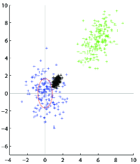
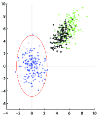
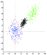
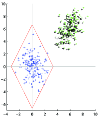
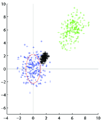
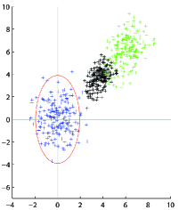
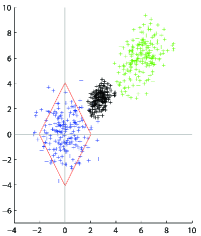
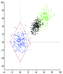
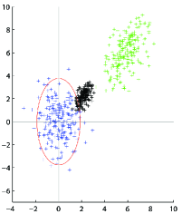
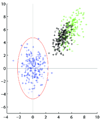
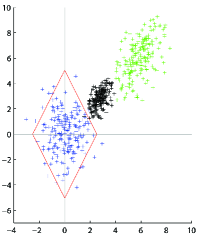
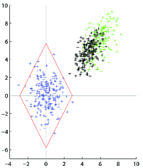
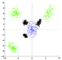
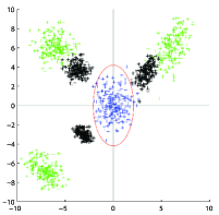
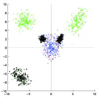
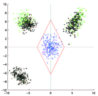
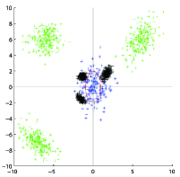
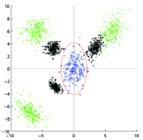
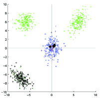
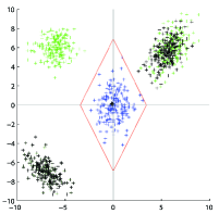
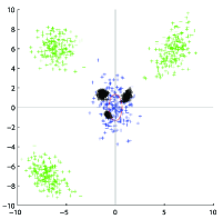
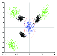
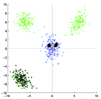
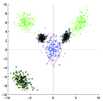
We consider two types of defensive walls around the centroids of the labeled normal objects. One is based on Euclidean distance (i.e., $L_{2}$ distance) and the other is based on Manhattan distance (i.e., $L_{1}$ distance). Left two plots of Fig. 1 show the Euclidean defensive walls, and the right two plots show the Manhattan defensive walls.

Based on Euclidean distance, the first type of defensive walls form an ellipsoid shaped region. Assume $p$ variables $X_{p\times 1}$ are joint normally distributed, the $(100\alpha)\%$ confidence region of $X$ ($0<\alpha<1$) is

$$(X-\vec{\mu})^{\prime}\Sigma^{-1}(X-\vec{\mu})=\chi^{2}_{p}(\alpha),$$

where $(X-\vec{\mu})^{\prime}\Sigma^{-1}(X-\vec{\mu})$ is weighted squared Euclidean distance. We compute the sample mean vectors $\hat{\mu}^{g}$ and the sample variance-covariance matrices $S^{g}$ of the objects in a labeled normal region from the first pass. Notice actual variables in a dataset need not follow multivariate normal distribution. Inspired by the above confidence region, we construct a Euclidean defensive wall as follows

$$(X-\hat{\mu}^{g})^{\prime}S^{g,-1}(X-\hat{\mu}^{g})=\chi^{2}_{p}(\alpha).$$

We choose the value of $\alpha$, $0<\alpha<1$, to control the size of an ellipsoid shaped defensive region.

The second type of defensive walls we use in our adversarial clustering technique is based on Manhattan distance. The Manhattan defensive walls form a diamond shaped region around the centroids of the normal regions. Here we compute the sample standard deviations $\hat{\sigma}^{g}_{i}$ and sample means $\hat{\mu}^{g}_{i}$ for each variable from the objects in a labeled normal region from the first pass. A Manhattan defensive wall is built as follows,

$$\sum_{i=1}^{p}\frac{|X_{i}-\hat{\mu}^{g}_{i}|}{\hat{\sigma}^{g}_{i}}=\eta.$$

The value of $\eta$ controls the size of a Manhattan defensive wall. The diamond shaped Manhattan defensive wall has vertices at $\hat{\mu}^{g}_{i}\pm\eta\hat{\sigma}^{g}_{i}$ along each dimension. $\eta$ can be expressed as a function of $\alpha$.

Compute $\eta(\alpha)$

We implement the following procedure to set the value of $\eta(\alpha)$ given an $\alpha$. Using the sample mean vector $\hat{\mu}^{g}$ and the sample variance-covariance matrix $S^{g}$ from the objects in a normal region, we generate a large sample from $N(\hat{\mu}^{g},S^{g})$. We then compute $\eta(\alpha)$ as a function of $\alpha$ ($0<\alpha<1$). For an $\eta(\alpha)$, $(100\alpha)\%$ of the generated sample points fall into the diamond shaped Manhattan region with vertices at $\hat{\mu}^{g}_{i}\pm\eta(\alpha)\hat{\sigma}^{g}_{i}$ on each dimension. Thus the values of $\eta(\alpha)$s are more closely spaced around the centroids for smaller $\alpha$s, and the spacing increases with bigger $\alpha$ values.

The sizes of the defensive walls are crucial. In Sec 3, we conduct a game theoretic study to provide guidelines about the equilibria $\alpha$s and $\eta(\alpha)$s under various attack scenarios.

Figure 1: One attacker with log utility function. Left to right: 1) Defender as Leader: $\alpha^{e}_{l}=0.29$, $t^{e}_{l}=0.78$; 2) Defender as Follower: $\alpha^{e}_{f}=0.95$, $t^{e}_{f}=0.20$; 3) Defender as Leader: $\eta^{e}_{l}=2.17$, $t^{e}_{l}=0.52$; 4) Defender as Follower: $\eta^{e}_{f}=3.33$, $t^{e}_{f}=0.03$

Figure 2: One attacker with linear utility function. Left to right: 1) Defender as Leader: $\alpha^{e}_{l}=0.46$, $t^{e}_{l}=0.72$; 2) Defender as Follower: $\alpha^{e}_{f}=0.85$, $t^{e}_{f}=0.39$; 3) Defender as Leader: $\eta^{e}_{l}=2.03$, $t^{e}_{l}=0.54$; 4) Defender as Follower: $\eta^{e}_{f}=2.52$, $t^{e}_{f}=0.34$

Figure 3: One attacker with exponential utility function. Left to right: 1) Defender as Leader: $\alpha^{e}_{l}=0.83$, $t^{e}_{l}=0.63$; 2) Defender as Follower: $\alpha^{e}_{f}=0.94$, $t^{e}_{f}=0.23$; 3) Defender as Leader: $\eta^{e}_{l}=2.52$, $t^{e}_{l}=0.53$; 4) Defender as Follower: $\eta^{e}_{f}=2.89$, $t^{e}_{f}=0.20$

3 A Game Theoretic Study for the Size of Defensive Walls

In this game theoretic study, we focus on how defender being a leader versus being a follower affects its equilibrium strategies, and consequently the sizes of equilibrium defensive walls. Often there are several non-cooperative adversaries that attempt to break through a defensive algorithm. Therefore we consider the following scenario. There is one defender with utility function $D(h)$, and there are $m$ adversaries, each with utility function $A_{i}(t_{i})$, $i=1,\cdots,m$. $h$ and $t_{i}$ are strategies in the corresponding players’ strategy spaces $H$ and $S_{i}$.

Assume the defender controls the normal population $\pi^{g}$, and each adversary controls a population $\pi^{b}_{i}$, $i=1,\cdots,m$. Each of the normal population and the adversaries’ populations may consist of multiple sub-populations, i.e. a player controlling a mixture population. Hence there may exist $g$ clusters of objects with $g\geq m+1$.

3.1 Adversarial Multi-Leader-Follower Stackelberg Game

As naturally the defender and the attackers observe each other’s actions, we model the scenario as an adversarial multi-leader-follower Stackelberg game. In the game the attackers and the defender act sequentially, one group being the leaders and another being the followers. The leaders choose their strategies first, and then after observing the leaders’ actions, the followers choose their strategies. Each follower maximizes its utility under the Cournot assumption that the other players hold their current strategy. Each leader acts considering the aggregate followers reaction, assuming no response from other leaders. Every player knows who are the leaders and who are the followers. And players have complete knowledge of each other.

Defender being the leader

This is a one-leader-m-follower game. Following the setup in [36, 37], we solve for an equilibrium of the game as follows.

1. Given a leader’s strategy $h$ fixed, assume the $m$ adversaries’ (i.e., the followers’) strategies are the attacks $T=(t_{1},\cdots,t_{m})$. For the $i$-th adversary, further assume all other adversaries’ strategies are fixed, i.e., fixed $t_{j}$, $\forall j\neq i$.

   Solve the following optimization for $t_{i}^{h}$:

   $$t_{i}^{h}=\text{argmax}_{\{t_{i}\in S_{i}\}}~{}~{}\{A_{i}(t_{i},h)\}$$

2. With the solution from above, $T^{h}=(t_{1}^{h},\cdots,t_{m}^{h})$ is the $m$ adversaries’ joint optimal attacks for a given defender strategy $h$, the defender solves another optimization problem.

   $$h^{e}=\text{argmax}_{\{h\in H\}}~{}~{}\{D(t_{1}^{h},\cdots,t_{m}^{h},h)\}$$

   Then $(h^{e},t_{1}^{h^{e}},\cdots,t_{m}^{h^{e}})$ is an equilibrium strategy for all players in the game.

In a Stackelberg game, the leader can predict the followers’ strategies and then decide its own optimal response. Hence this can be interpreted as the defender sets the equilibrium for all players in the game.

Defender being the follower

This becomes a m-leader-one-follower game. Following the setup in [39], which is an extension of [36, 37], we solve for an equilibrium of the game as follows.

1. Given the joint attacks from the $m$ adversaries, $T=(t_{1},\cdots,t_{m})$, solve for the defender’s optimal strategy.

   $$h_{T}=\text{argmax}_{\{h\in H\}}~{}~{}\{D(t_{1},\cdots,t_{m},h)\}$$

2. With the solution above as the defender’s optimal strategy $h_{T}$ against joint attacks $T=(t_{1},\cdots,t_{m})$, solve for the optimal joint attacks $T^{e}$.

   $$T^{e}=(t_{1}^{e},...,t_{m}^{e})=\text{argmax}_{\{t_{i}\in S_{i},\forall i\}}{\sum_{i=1}^{m}A_{i}(t_{i},h_{T})}$$

   Then $(h^{T^{e}},t_{1}^{e},\cdots,t_{m}^{e})$ is an equilibrium strategy for all players in the game.

The attackers as a whole are the leaders in the game. They act non-cooperatively to choose their strategies. The attackers in this setup can be very different from one another. Together they set the equilibrium of the Stackelberg game.

To find an equilibrium, the defender being either the leader or the follower in the game, is to solve these optimization problems. Next in Section 3.2, we provide a concrete setup of the games and define the attackers’ strategy spaces and the defender’s strategy space. We obtain approximate solutions to these optimization problems by performing exhaustive search. We divide the attacker’s strategy spaces into fine grids (e.g., attack strength $t$ over fine grids from 0 to 1 by 0.01 for every attacker), and defender’s strategy space into fine grids (e.g., defensive wall size $\alpha$ over fine grids from 0 to 1 by 0.01 for defender). We then search over the fine grids. Even with a large number of attackers, it is computationally feasible to perform such exhaustive search. The solution is an accurate approximate equilibrium of a game.

Figure 4: Three attackers each with log utility functions. Left to right: 1) Defender as Leader: $\alpha^{e}_{l}=0.71$, $\vec{t}^{e}_{l}=(0.58,0.65,0.59)$; 2) Defender as Follower: $\alpha^{e}_{f}=0.89$, $\vec{t}^{e}_{f}=(0.43,0.56,0.39)$; 3) Defender as Leader: $\eta^{e}_{l}=1.63$, $\vec{t}^{e}_{l}=(0.66,0.00,0.67)$; 4) Defender as Follower: $\eta^{e}_{f}=3.16$, $\vec{t}^{e}_{f}=(0.11,0.00,0.13)$

Figure 5: Three attackers each with linear utility functions. Left to right: 1) Defender as Leader: $\alpha^{e}_{l}=0.38$, $\vec{t}^{e}_{l}=(0.72,0.78,0.78)$; 2) Defender as Follower: $\alpha^{e}_{f}=0.88$, $\vec{t}^{e}_{f}=(0.44,0.58,0.45)$; 3) Defender as Leader: $\eta^{e}_{l}=0.35$, $\vec{t}^{e}_{l}=(0.91,0.00,0.94)$; 4) Defender as Follower: $\eta^{e}_{f}=3.45$, $\vec{t}^{e}_{f}=(0.08,0.00,0.98)$

Figure 6: Three attackers each with exponential utility functions. Left to right: 1) Defender as Leader: $\alpha^{e}_{l}=0.20$, $\vec{t}^{e}_{l}=(0.80,0.89,0.78)$; 2) Defender as Follower: $\alpha^{e}_{f}=0.89$, $\vec{t}^{e}_{f}=(0.44,0.58,0.41)$; 3) Defender as Leader: $\eta^{e}_{l}=0.56$, $\vec{t}^{e}_{l}=(0.86,0.01,0.88)$; 4) Defender as Follower: $\eta^{e}_{f}=1.85$, $\vec{t}^{e}_{f}=(0.52,0.01,0.58)$

3.2 Attacks Under Gaussian Mixture Populations

We then consider the following attack scenario to obtain important insights about how large the defensive walls become at an equilibrium and how they are affected by the defender’s role in the game. Assume $p$ variables are measured from each object, $X=(X_{1},...,X_{p})$. First assume every population follows a single multivariate Gaussian distribution. Let the normal population $\pi^{g}$ follows $N_{p}(\mu^{g},\Sigma^{g})$. Let an adversarial population $\pi^{b}_{i}$ follows $N_{p}(\mu^{b}_{i},\Sigma^{b}_{i})$ before launching attacks.

When an adversary launches an attack $t$, it moves the objects under its control toward $\mu^{g}$, the center of the normal population. An object $X$ is transformed by attack $t$ and becomes

$$X^{t}=\mu^{g}+(1-t)\times(X-\mu^{g}).$$

Notice $0\leq t\leq 1$. $t=1$ is the strongest attack, since all the transformed objects equal to $\mu^{g}$, the center of the normal population, and $t=0$ means no attack. Under attack $t$, the population controlled by an adversary becomes

$$N((1-t)\mu^{b}+t\mu^{g},~{}~{}(1-t)^{2}\Sigma^{b}).$$

Here we consider the scenario where the objects under the adversary’s control are moved by the same factor $t$.

The joint attack from the $m$ adversaries, i.e. the adversaries’ strategies, is then $(t_{1},\cdots,t_{m})$, $\forall t_{i}\in[0,1]$. The defender’s strategy is to build a defensive wall around the center $\mu^{g}$ of its population. A Euclidean defensive wall is controlled by a factor $\alpha$ and a Manhattan defensive wall is controlled by $\eta(\alpha)$, $\alpha\in(0,1)$. Hence a defender’s strategy is $h=\alpha$ or $h=\eta(\alpha)$, depending on the type of defensive walls it uses.

3.3 Utility Functions

In this game theoretic study, we define the defender’s utility based on error rates of normal objects and adversary objects, which are between 0 and 1, and their corresponding misclassification costs. We let the misclassification cost of normal objects to be 1 and the misclassification cost of adversary objects to be $c$. It is multiplied by $-100$ so that the defender tries to maximize its utility in the game.

$$D(h)=-100(\text{error-of-normal}+c\times\text{error-of-adversary})$$

Defender utility $D(h)$ is equivalent to $D(\alpha)$ or $D(\eta(\alpha))$, since error rates are functions of $\alpha$ or $\eta(\alpha)$.

Let $k$ be the maximum utility of an adversary object when it passes a defensive algorithm without the need of being modified. $||X^{t}-X||_{2}$, the $L_{2}$ distance between the original object and the modified object once an attack $t$ is launched, measures how much an adversary object is moved towards normal. The minimum utility of an adversary object is 0, either caused by heavy modification or being blocked by the defensive algorithm. Moving an adversary object towards normal is penalized. For the adversaries, we consider three utility functions with increasing level of penalties for launching an attack. The three utility functions are the expected values of a penalized adversary object if it passes the defensive algorithm after being moved towards normal. An adversary’s log utility function is defined as

$$G(t)=E\left(\text{max}\{k-a\times\log{(||X^{t}-X||_{2}+1)},0\}\right).$$

An adversary’s linear utility function is defined as

$$L(t)=E\left(\text{max}\{k-a\times||X^{t}-X||_{2},0\}\right).$$

An adversary’s exponential utility function is defined as

$$E(t)=E\left(\text{max}\{k-\text{exp}(a\times||X^{t}-X||_{2}),0\}\right).$$

In the adversarial multi-leader-follower Stackelberg game, all the players, the defender and the adversaries, choose their strategies to maximize their utilities. For the defender, it is equivalent to minimize its overall misclassification cost. For the adversaries, it is to maximize the expected utilities of the unblocked attack objects.

3.4 Simulations

Notice the defender strategy is either to choose $\alpha$ or $\eta(\alpha)$ which controls its defensive wall, and an adversary’s strategy is an attack $t$, where $0<\alpha<1$ and $0\leq t\leq 1$. By performing exhaustive search over fine grids of $\alpha$ (or $\eta(\alpha)$) and $t_{i}$, we can find the approximate equilibrium in a game. Here we conduct experiments to examine the equilibrium strategies of the defender and the adversaries under different settings.

Simulations With One Adversary

There is only one adversary in the first set of experiments. Both normal and adversary populations follow bivariate normal distributions. Let the normal population have $\mu^{g}=(0,0)$ and $\Sigma^{g}=\begin{bmatrix}1&0\\ 0&2\end{bmatrix}$. Without an attack, let the adversary population original $\mu^{b}=(6,6)$ and $\Sigma^{b}=\begin{bmatrix}1&1\\ 1&2\end{bmatrix}$.

Defender error cost $c=20$ in Figures 1, 2, 3. The blue ’+’s are the normal objects, the green ’+’s are the original adversary objects, and the black ’+’s are the moved adversary objects in an attack. Without an attack, the normal and the adversary populations are well separated and the defender can easily build a defensive line. The adversary has a log utility with $a=4$ for Figure 1; it has a linear utility with $a=1.5$ for Figure 2; and an exponential utility with $a=0.75$ for Figure 3. Figures 1, 2, 3 show when defender being the leader vs being the follower, how large is its Euclidean (red ellipsoid) and Manhattan (red diamond) defensive walls and the strength of the corresponding attacks at the equilibrium.

Remark: We observe that when defender is the leader, it tends to choose a much more conservative strategy with a smaller defensive wall. In turn the adversaries launch stronger attacks to break into the defensive walls. The strength of penalties on attacks significantly affects the adversaries’ strategies, while the misclassification cost is a key factor for the defender to choose its strategy.

Simulations With Three Adversaries

There are three adversaries in the second set of experiments. Normal and adversary populations follow bivariate normal distributions for Figures 4, 5, 6. The normal population has $\mu^{g}=(0,0)$ and $\Sigma^{g}=\begin{bmatrix}1&0\\ 0&2\end{bmatrix}$. Without an attack, the first adversary population originally has $\mu^{b}_{1}=(6,6)$ and $\Sigma^{b}_{1}=\begin{bmatrix}1&1\\ 1&2\end{bmatrix}$. The second adversary population originally has $\mu^{b}_{2}=(-7,-7)$ and $\Sigma^{b}_{2}=\begin{bmatrix}1&-0.5\\ -0.5&1\end{bmatrix}$. The third adversary population originally has $\mu^{b}_{3}=(-6,6)$ and $\Sigma^{b}_{3}=\begin{bmatrix}1&0\\ 0&2\end{bmatrix}$. We let $k=7$ and $c=10$. For Figure 4, we have $(a_{1},a_{2},a_{3})=(1.75,1.25,.1.25)$ for three adversary log utility functions. For Figure 5, we have $(a_{1},a_{2},a_{3})=(0.5,0.25,0.5)$ for three adversary linear utility functions. For Figure 6, we have $(a_{1},a_{2},a_{3})=(4.5,4,4.5)$ for three adversary exponential utility functions.

We observe that Euclidean defensive walls used by the defender tends to encourage attacks with similar strength. Given the initial position of different adversaries and their penalties, Manhattan defensive walls used by the defender can discourage an adversary from launching an attack.

Remark: When defender is the follower, it is able to observe the action of the attackers and hence draw a less conservative defensive wall. In our ADClust algorithm, we choose to take the follower approach. We recommend $\alpha$ in the range from 0.6 to 0.8 following the game theoretic simulations. Hence we identify the centers of normal without blocking out too many normal objects or even letting the adversaries to launch strong attacks.

Figure 7: Left to right: 1) Simulation 1 true labels; 2) Simulation 2 true labels; 3) Simulation 3 true labels;

Figure 8: Simulation 1 comparison with $\alpha=0.6$. Left to right: 1) ADClust with $k=10$; 2) ADClust with $k=20$; 3) EM least square; 4) S4VM

Figure 9: Simulation 2 comparison with $\alpha=0.6$. Left to right: 1) ADClust with $k=10$; 2) ADClust with $k=20$; 3) EM least square; 4) S4VM

Figure 10: Simulation 3 comparison with $\alpha=0.6$. Left to right: 1) ADClust with $k=10$; 2) ADClust with $k=20$; 3) EM least square; 4) S4VM

Figure 11: Quantitative measures as the weight $k$ increases from 1 to 100. Left Column: Top panel is percent of abnormal points in mixed region and bottom panel is percent of abnormal points among outliers; Right Column: Top panel is the number of points in mixed region and bottom panel is the number of points as outliers.

Figure 12: Left Panel: The boxplots of percent of normal objects within Manhattan defensive walls with different $\alpha$ levels and weight $k$. The corresponding $\eta(\alpha)$ values are 5.89, 7.25, 8.97, 11.51, 13.72; Right Panel: The boxplots of percent of normal objects within Euclidean defensive walls with different $\alpha$ levels and weight scalars.

4 Experiments

4.1 Simulated Experiment

We conduct three simulations to compare our ADClust with two semi-supervised learning algorithms, EM least square [25] and S4VM [27]. In all three simulations, we generate data points from several bivariate normal distributions. The bivariate normal distributions have the same variance-covariance matrix

$$\Sigma=\begin{bmatrix}0.4&0\\ 0&0.4\end{bmatrix}.$$

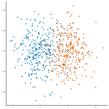
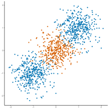
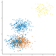
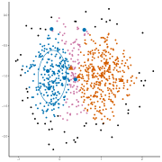
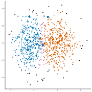
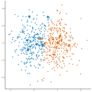
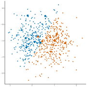
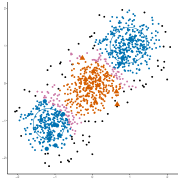
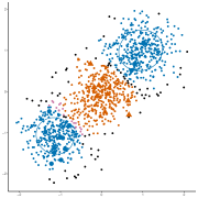
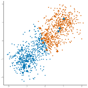
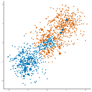
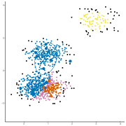
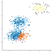
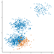
Figure 7 shows the true labels of the points for the three simulations. Solid triangles and solid circles are the 2% labeled points. Figures 8, 9, and 10 show the comparison results. We set $\alpha=0.6$. Blue dots are used for normal points, either true or labeled. Orange dots are used for abnormal points, either true or labeled. Purple dots are for unlabeled points in mixed regions. Yellow dots are for unknown unlabeled clusters. Black dots are for unlabeled outliers. Different regions are marked using different colors.

In these three simulations, we show the data points after attacks have taken place. In Simulation 1 previously separated normal and abnormal clusters now have overlapped areas and are merged into one big cluster. In Simulation 2, an attack takes place between two normal regions, and attack objects manage to mix three clusters into one big cluster. Simulation 3 suffers the strongest attack, where normal and abnormal clusters are heavily mixed. There is also a previously unknown cluster in simulation 3, which cannot be identified as either normal or abnormal at the training time, potentially a new attack.

Defensive walls, studied under a game theoretic framework, are a crucial factor in our algorithm. With wall size $\alpha=0.6$, as in the recommended range from the game theoretic study considering defender being a follower, the defensive walls mark out the center areas of the normal regions with nearly pure normal objects in Simulation 1 and 2, where attacks have not yet reached the centers of the normal. In Simulation 2, the defensive walls in our ADClust algorithm successfully mark out the two centers of the two normal regions. On the other hand the semi-supervised learning algorithms still make a hard separation of normal vs. abnormal. One normal cluster is completely wrongly labeled by the two semi-supervised learning algorithms. In Simulation 3, our algorithm leaves an previously unknown cluster unlabeled. It needs to be examined carefully later since it can potentially be a new attack. The two semi-supervised learning algorithms label the unknown cluster as normal, making a high risk decision.

Simulation 1: There are two sets of random samples generated from two bivariate normal distributions, centered at (0, -1) (normal class), and (1, -1) (abnormal class) respectively. Each has 300 data points. We random select $2\%$ of the points and save their labels. EM least square and S4VM make a hard separation, and try their best to label all the points in the mixed region. Hence they make noticeable mistakes in the mixed region. Our ADClust does not assign class labeled to the points in the mixed region. We instead mark out the whole region. The comparison between our marked mixed region and a classification boundary is similar to a confidence band vs a point estimate. We also identify and leave outliers unlabeled, as shown in Figure 8.

Simulation 2: There are three sets of random samples generated from three bivariate normal distributions, centered at (-1, -1) (abnormal class), (0, 0) (normal class), and (1, 1) (abnormal class) respectively. Each has 300 data points. We random select $2\%$ of the points and save their labels. EM least square and S4VM divide the big cluster into two areas. They fail to distinguish three overlapping clusters. Our ADClust is able to identify the three clusters and mark out the two mixed regions, without assigning class labels there, as shown in Figure 9.

Simulation 3: There are four sets of random samples generated from four bivariate normal distributions, centered at (0.5, -1) (normal class), (1, -1) (abnormal class), (1, 1) (normal class), and (3, 3) (unknown class). They have 300, 300, 300, 100 data points respectively. We random select $2\%$ of the points from only normal and abnormal classes and save their labels. The unknown class has no labeled point. EM least square and S4VM label the unknown cluster as normal, where there is no reliable information. Furthermore, their assigned labels are highly inaccurate in the mixed regions. Our ADClust leave out the unknown cluster as unlabeled, and identify the mixed region without assigning labels there, as shown in Figure 10.

In the three simulations, we use two weight values. $k=10$ and $k=20$. A smaller weight $k$ is a more conservative strategy, i.e., we get smaller labeled regions and a larger unlabeled mixed region. On the other hand, if we use a larger weight $k$, it is a more aggressive strategy. We expect larger labeled regions and smaller unlabeled mixed region. Drawing defensive walls following the game theoretic study correctly identify the normal centers, while semi-supervised learning algorithms completely fail to do so under certain scenarios.

4.2 KDD Cup 1999 Data

The KDD cup 1999 data was initially created by MIT Lincoln Labs [23]. The full dataset contains about 126k labeled objects for training purpose. Around 40 percent of the objects are network intrusion instances. There are 41 features for each object. [1] ranked the 41 features with respect to their effectiveness in separating normal instances from abnormal instances. We use the KDD Cup 99 data to demonstrate how our ADClust algorithm performs. We take 25192 instances from training set. We include top 7 continuous features according to [1] for each instance.

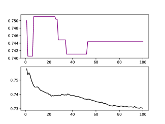
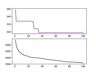
In the first experiment, in a single run, we randomly sample 150 instances and keep their labels. The rest are treated as unlabeled instances in the run. We perform 100 runs. An overwhelming majority (i.e., 99.4%) of the instances are unlabeled.

We gradually increase the weight $k$ from 1 to 100. Along with the increasing weight, we have less unlabeled points. As a result, it is a more aggressive strategy. Meanwhile, the normal region increases and it includes more points which are more likely to be mis-labeled abnormal objects. Therefore, we have a trade-off in choosing weight $k$. It is a trade-off between the size of the labeled regions within a cluster and the error rate of mis-labeled points. In Figure 11, the number of points in mixed regions and outliers decreases as we have a larger weight. The percentage of abnormal objects in the mixed areas and among outliers decreases from 76% to 73% as the weight $k$ increases, which means we have to exam the mixed areas very carefully.

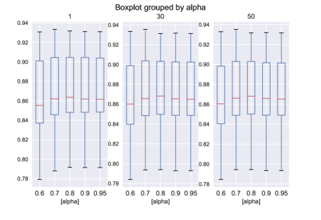
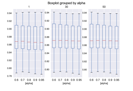
In a second experiment, we draw two boxplots to show the percent of normal objects (i.e., the success rate) within the defensive walls as shown in Figure 12. We again have 100 runs. For each run, we randomly select 100 points to keep their labels. Based on the labels, we perform ADClust to cluster instances. Then we set different weights and examine different alpha levels for the defensive walls. We set $k$ to 1, 30 and 50 as low, medium and high weights. For each of the weight, we show the success rates for the two types of defensive walls.

We set $\alpha$ levels from 0.6 to 0.95. The median of the success rates varies from 0.85 to 0.87. We find that the weights $k=30$ and $k=50$ perform better than $k=1$ in term of success rate. Furthermore, $\alpha=0.8$ has the highest median success rate for Manhattan defensive walls and $\alpha=0.7$ has the highest median success rate for Euclidean defensive walls. Both of the results are consistent with the recommended $\alpha$ range, 0.6 to 0.8, from the game theoretic studies.

Note semi-supervised learning techniques are designed to achieve the highest overall accuracy over all unlabeled normal and abnormal objects. On the other hand, our algorithm does keep many points unlabeled, hence we do not have an overall accuracy measure computed over all the unlabeled objects. Meanwhile one of our algorithm’s focus is to have objects as purely normal inside the defensive walls as possible, at the expense of decreased accuracy, since many normal objects are blocked out of the wall along with the abnormal ones. In this experiment, KDD data is a highly mixed data, yet we achieve on average nearly 90% pure normal rate inside the defensive walls, marked as the relatively safe regions. The unlabeled mixed regions, and unlabeled whole clusters if there is any, are another focus of our algorithm. Results from our algorithm can be used for tiered screenings of the objects, with the objects in the mixed region examined most carefully to separate normal from abnormal, and the unknown clusters examined for potential new attacks.

5 Conclusion

In this paper, we develop a novel adversarial clustering algorithm, a.k.a. ADClust, to separate the attack region and the normal region within mixed clusters caused by adversaries’ attack objects. With very few labeled instances, we cannot build an effective classifier, which has a clearly defined classification boundary to defend the normal population from the attack objects. However utilizing the few labeled objects, our clustering algorithm can identify the mixed area between the normal region and the attack region. Instead of a classifier boundary, analogous to a point estimate, an overlapping area is analogous to a confidence region, showing the strength of an attack. Furthermore defensive walls are drawn inside normal regions. This is a conservative strategy to defend the normal population against active adversaries. All objects outside the centers of the normal objects need to be examined carefully, especially in the mixed regions.

Acknowledgements This work is supported in part by ARO grant W911NF-17-1-0356, NIH award 1R01HG006844 and NSF CNS-1111529, CNS-1228198, CICI-1547324, and IIS-1633331.

References

- [1] Ammar, A. and Al-Shalfan, K., Neural Networks Based Feature Selection from KDD Intrusion Detection Dataset. In New Developments in Computational Intelligence and Computer Science
- [2] Basu, S., Bilenko, M., and Mooney, R. J. (2004). A probabilistic framework for semi-supervised clustering. In Proceedings of the tenth ACM SIGKDD international conference on Knowledge discovery and data mining, 59–68
- [3] Balcan, M. F., and Blum, A. (2005). A PAC-Style Model for Learning from Labeled and Unlabeled Data. In COLT, 111–126.
- [4] Biggio, B., Pillai, I., Rota Bulò, S., Ariu, D., Pelillo, M. and Roli, F. (2013). Is data clustering in adversarial settings secure?. In Proceedings of the 2013 ACM workshop on Artificial intelligence and security, 87-98.
- [5] Biggio, B., Bulò, S.R., Pillai, I., Mura, M., Mequanint, E.Z., Pelillo, M. and Roli, F. (2014). Poisoning complete-linkage hierarchical clustering. In Joint IAPR International Workshops on Statistical Techniques in Pattern Recognition (SPR) and Structural and Syntactic Pattern Recognition (SSPR) 42–52
- [6] Bilenko, M., Basu, S., and Mooney, R. J. (2004). Integrating constraints and metric learning in semi-supervised clustering. In Proceedings of the twenty-first international conference on Machine learning, p.11
- [7] Bilenko, M., and Mooney, R. J. (2003). Adaptive duplicate detection using learnable string similarity measures. In Proceedings of the ninth ACM SIGKDD international conference on Knowledge discovery and data mining, 39–48
- [8] Bohm, C., and Plant, C. (2008). Hissclu: a hierarchical density-based method for semi-supervised clustering. In Proceedings of the 11th international conference on Extending database technology: Advances in database technology, 440–451
- [9] Bruckner, M. and Scheffer, T. (2011). Stackelberg games for adversarial prediction problems. In Proceedings of the 17th ACM SIGKDD international conference on Knowledge discovery and data mining, 547–555
- [10] Chapelle, O., and Zien, A. (2005). Semi-supervised classification by low density separation. In AISTATS, 57–64.
- [11] Collins, M., and Singer, Y. (1999). Unsupervised models for named entity classification. In Proceedings of the joint SIGDAT conference on empirical methods in natural language processing and very large corpora, 100–110.
- [12] Cozman, F. G., Cohen, I., and Cirelo, M. C. (2003). Semi-supervised learning of mixture models. In Proceedings of the 20th International Conference on Machine Learning, 99–106.
- [13] Culp, M., and Michailidis, G. (2008). An iterative algorithm for extending learners to a semi-supervised setting. Journal of Computational and Graphical Statistics, 17(3), 545–571.
- [14] Dalvi, N., Domingos, P., Sanghai, S. and Verma, D. (2004), Adversarial classification. In Proceedings of the tenth ACM SIGKDD international conference on Knowledge discovery and data mining, 99–108
- [15] Dekel, O., Shamir, O. and Xiao, L. (2010). Learning to classify with missing and corrupted features. Machine learning, 81(2), 149–178.
- [16] Dutrisac, J.G. and Skillicorn, D.B. (2008). Hiding clusters in adversarial settings. In 2008 IEEE International Conference on Intelligence and Security Informatics, 185–187.
- [17] Ester, M., Kriegel, H.P., Sander, J. and Xu, X. (1996). A density-based algorithm for discovering clusters in large spatial databases with noise. In Kdd 1996, Vol. 96, No. 34, 226–231.
- [18] Fujino, A., Ueda, N., and Saito, K. (2005). A hybrid generative/discriminative approach to semi-supervised classifier design. In AAAI, 764–769.
- [19] Haffari, G. R., and Sarkar, A. (2012). Analysis of semi-supervised learning with the yarowsky algorithm. arXiv preprint arXiv:1206.5240.
- [20] Huang, L., Joseph, A.D., Nelson, B., Rubinstein, B.I. and Tygar, J.D. (2011). Adversarial machine learning. In Proceedings of the 4th ACM workshop on Security and artificial intelligence, 43–58
- [21] Kantarcioglu, M., Xi, B. and Clifton, C. (2011). Classifier evaluation and attribute selection against active adversaries. Data Mining and Knowledge Discovery, 22(1-2), 291–335.
- [22] Klein, D., Kamvar, S. D., and Manning, C. D. (2002). From instance-level constraints to space-level constraints: Making the most of prior knowledge in data clustering. Stanford.
- [23] Knowledge discovery in databases DARPA archive. TaskDescription. http://www.kdd.ics.uci.edu/databases/kddcup99/task.html
- [24] Kearns, M. and Li, M. (1993). Learning in the presence of malicious errors. SIAM Journal on Computing, 22(4), 807–837.
- [25] Krijthe, J.H. and Loog, M., 2016, December. Optimistic semi-supervised least squares classification. In 2016 23rd International Conference on Pattern Recognition (ICPR), 1677–1682
- [26] Lelis, L., and Sander, J. (2009). Semi-supervised density-based clustering. In ICDM’09, 842–847
- [27] Li, Y.F. and Zhou, Z.H., 2015. Towards making unlabeled data never hurt. IEEE Transactions on Pattern Analysis and Machine Intelligence, 37(1), 175–188.
- [28] L’Huillier, G., Weber, R. and Figueroa, N. (2009). Online phishing classification using adversarial data mining and signaling games. In Proceedings of the ACM SIGKDD Workshop on CyberSecurity and Intelligence Informatics, 33–42
- [29] Lowd, D. and Meek, C. (2005). Adversarial learning. In Proceedings of the eleventh ACM SIGKDD international conference on Knowledge discovery in data mining, 641–647
- [30] N. MacDonald, Information Security Is Becoming a Big Data Analytics Problem, https://www.gartner.com/doc/1960615/ information-security-big-data-analytics
- [31] McCallum, A., and Nigam, K. (1998). A comparison of event models for naive bayes text classification. In AAAI-98 workshop on learning for text categorization, Vol. 752, 41–48
- [32] Nigam, K., McCallum, A. K., Thrun, S., and Mitchell, T. (2000). Text classification from labeled and unlabeled documents using EM. Machine learning, 39(2), 103-134.
- [33] Ratsaby, J., and Venkatesh, S. S. (1995). Learning from a mixture of labeled and unlabeled examples with parametric side information. In Proceedings of the eighth annual conference on Computational learning theory, 412–417
- [34] Rosenberg, C., Hebert, M., and Schneiderman, H. (2005). Semi-supervised self-training of object detection models.
- [35] Rubinstein, B.I., Nelson, B., Huang, L., Joseph, A.D., Lau, S.H., Rao, S., Taft, N. and Tygar, J.D. (2009). Antidote: understanding and defending against poisoning of anomaly detectors. In Proceedings of the 9th ACM SIGCOMM conference on Internet measurement conference, 1–14
- [36] Sherali, H. D., Soyster, A. L., Murphy, F. H. (1983). Stackelberg-Nash-Cournot equilibria: characterizations and computations. Operations Research, 31(2), 253-276.
- [37] Sherali, H. D., (1984). A Multiple Leader Stackelberg Model and Analysis. Operations Research, 32(2), 390–404.
- [38] Sindhwani, V., and Keerthi, S. S. (2006). Large scale semi-supervised linear SVMs. In Proceedings of the 29th annual international ACM SIGIR conference on Research and development in information retrieval, 477–484.
- [39] Sinha, A., Malo, P., Frantsev, A. and Deb, K. (2014). Finding optimal strategies in a multi–period multi–leader–-follower Stackelberg game using an evolutionary algorithm. Computers & Operations Research, 41, 374–385.
- [40] Stein, T., Chen, E. and Mangla, K. (2011). Facebook immune system. In Proceedings of the 4th Workshop on Social Network Systems (p. 8). ACM.
- [41] Wang, Y.X. and Xu, H. (2013). Noisy Sparse Subspace Clustering. In ICML (1), 89–97.
- [42] Wagstaff, K., Cardie, C., Rogers, S., and Schrödl, S. (2001). Constrained k-means clustering with background knowledge. In ICML, Vol 1, 577–584.
- [43] Xing, E. P., Jordan, M. I., Russell, S. J., and Ng, A. Y. (2003). Distance metric learning with application to clustering with side-information. In Advances in neural information processing systems, 521–528.
- [44] Yanchang, Zhao, and Song Junde. ”GDILC: a grid-based density-isoline clustering algorithm.” Info-tech and Info-net, 2001. Proceedings. ICII 2001-Beijing. 2001 International Conferences on. Vol. 3. IEEE, 2001.
- [45] Zhang, T., and Oles, F. (2000). The value of unlabeled data for classification problems. In Proceedings of the Seventeenth International Conference on Machine Learning, 1191–1198.
- [46] Zhou, Z. H., Zhan, D. C., and Yang, Q. (2007). Semi-supervised learning with very few labeled training examples. In AAAI, 675–680.
- [47] Zhou, Y., Kantarcioglu, M., Thuraisingham, B. and Xi, B. (2012). Adversarial support vector machine learning. In Proceedings of the 18th ACM SIGKDD international conference on Knowledge discovery and data mining, 1059–1067