Binary companions of evolved stars in APOGEE DR14:
Search method and catalog of $\sim$5,000 companions

Abstract

Multi-epoch radial velocity measurements of stars can be used to identify stellar, sub-stellar, and planetary-mass companions. Even a small number of observation epochs can be informative about companions, though there can be multiple qualitatively different orbital solutions that fit the data. We have custom-built a Monte Carlo sampler (The Joker) that delivers reliable (and often highly multi-modal) posterior samplings for companion orbital parameters given sparse radial-velocity data. Here we use The Joker to perform a search for companions to 96,231 red-giant stars observed in the APOGEE survey (DR14) with $\geq 3$ spectroscopic epochs. We select stars with probable companions by making a cut on our posterior belief about the amplitude of the stellar radial-velocity variation induced by the orbit. We provide (1) a catalog of 320 companions for which the stellar companion properties can be confidently determined, (2) a catalog of 4,898 stars that likely have companions, but would require more observations to uniquely determine the orbital properties, and (3) posterior samplings for the full orbital parameters for all stars in the parent sample. We show the characteristics of systems with confidently determined companion properties and highlight interesting systems with candidate compact object companions.

Section 1 Introduction

Time-domain radial-velocity measurements of stars contain information about massive companions. Even with two successive observations of a single star, a difference in the measured radial velocities implies the existence of at least one companion. However, with few or imprecise radial-velocity measurements, the orbital properties of the companion(s) may be poorly constrained (e.g., Price-Whelan et al. 2017). The vast majority of spectroscopic targets with repeat observations in the largest (by number of objects) stellar spectroscopic surveys are observed just a few times with sparse, non-uniform phase coverage. Most prior searches for companions using survey RV data have therefore restricted their searches to only sources with many, high-precision epochs, so that the orbital solution can be unambiguously determined (e.g., Troup et al. 2016), or have used simple statistics computed from the data to study multiplicity (e.g., $\textrm{RV}_{\textrm{max}}$; Badenes et al. 2017).

If there are only a few radial-velocity epochs per star, and if the companion spectrum is not observed, the data will be consistent with many different combinations of primary orbital parameters (period, amplitude, eccentricity, etc.). To identify companions to the typical star observed in a spectroscopic survey, we therefore face at least one major challenge: how, given a small number of observations of a primary star, do we reliably obtain posterior information about the binary-system properties? In general, the likelihood function—and the posterior probability distribution function (pdf) under any reasonable prior pdf—will be highly multimodal, and many of the modes will have comparable integrated probability density. For example, with just two radial-velocity measurements, a harmonic series of period modes will exist in the likelihood function.

We have solved the problem of deriving comprehensive multi-modal pdf samplings previously with The Joker (Price-Whelan et al. 2017), a Monte Carlo rejection sampler that is computationally expensive but probabilistically righteous: It delivers independent posterior pdf samples for single-companion binary orbital parameters, given any number of radial-velocity measurements. Here we use The Joker to generate posterior pdf samples for stars observed by the APOGEE survey (see Section 2; Majewski et al. 2017).

The APOGEE surveys primarily target red-giant-branch (RGB) and other evolved stars (e.g., red clump giants, RC), which are ideal for the study of single-line binary systems. In general, they are unlikely to have comparably-bright companions, and their spectra are therefore fit as single-line objects. When this constraint is not met, The Joker will in general fail, and a model that fits for a mixture of stellar spectra is more appropriate (e.g., El-Badry et al. 2018). The subset of RC stars are even more powerful as they are standard candles and have masses that can be estimated using spectroscopy (using dredged-up elements; Martig et al. 2016; Ness et al. 2016). With mass estimates for the primary star, the binary-orbit fitting will return $M_{2}\,\sin i$ (minimum mass) estimates for the secondary, and not just estimates of the so-called “binary mass function.” Additionally, the APOGEE pipelines (García Pérez et al. 2016a) and also The Cannon (Ness et al. 2015) produce detailed abundance estimates for RGB and RC stars. If there are causal relationships between chemical abundances and binary companions—as are expected—these should be measurable.

By making cuts on this library of posterior pdf samples (described in detail in Section 5), we deliver catalogs of binary-star systems from the APOGEE survey, and show the bulk properties of these systems.

Binary and multiple star systems are of great interest in astrophysics: The population of stars and their companions encodes information about star formation processes, stellar parameters and evolution, and the dynamics of multi-body systems (for recent reviews, see Duchêne & Kraus 2013; Moe & Di Stefano 2017). Most of what is known about stellar companions comes from studies of nearby main-sequence (MS) stars (e.g., Duquennoy et al. 1991; Raghavan et al. 2010; Tokovinin 2014; Moe & Di Stefano 2017). Nearly 50% of MS stars in the solar neighborhood have companions (e.g., Tokovinin 2014). MS stars with companions have a large dynamic range of constituent and orbital characteristics. For example, binary stars have mass-ratios that span from $\approx 0.03$ to 1 (e.g., Kraus et al. 2008), and have periods from days to millions of years (e.g., Raghavan et al. 2010). Less is known about population properties of non-interacting or detached companions to evolved stars. The catalogs and methodology presented in this work are a first step towards performing population inferences of binary star systems with evolved star members.

Section 2 Data

All data used in this work come from the publicly-available data release 14 (DR14) of the APOGEE survey (Majewski et al. 2017; Abolfathi et al. 2017), a component of the Sloan Digital Sky Survey IV (SDSS-IV; Gunn et al. 2006; Blanton et al. 2017). APOGEE is designed to map stars across much of the Milky Way by obtaining high-resolution ($R\sim 22,500$) infrared ($H$-band) spectroscopy of primarily RGB stars. Targets are selected with simple color and brightness cuts, but the survey uses fiber-plugged plates with a maximum of 300 fibers per each $\approx 1.5~{}\textrm{deg}^{2}$ field of view, leading to “pencil-beam”-like sampling of the Galactic stellar distribution. In order to meet signal-to-noise ratio requirements, most APOGEE stars are observed multiple times in a series of “visits,” typically with at least one visit separated by a month or more in order to help identify binary stars.

Data taken as part of the APOGEE survey are reduced with a multi-step data reduction pipeline that ultimately solves for the stellar parameters, chemical abundances, and radial velocities for each target (Nidever et al. 2015). Most relevant for this work, the visit radial velocities (RVs) are determined using an iterative scheme: the individual visit spectra are combined using initial guesses for the relative RVs into a coadded spectrum, which is then used to re-derive the relative visit velocities. The stellar parameters—surface gravity, $\log g$, and effective temperature, $T_{\textrm{eff}}$—and the chemical abundances are determined from the coadded spectrum as a part of the APOGEE Stellar Parameters and Chemical Abundances Pipeline (ASPCAP; García Pérez et al. 2016b).

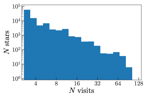
Figure 1: Number of APOGEE DR14 stars in logarithmic bins of number of visits that pass the quality cuts described in Section 2. In total, this work uses 397,559 visits and 96,231 unique sources.

We use the primary data products from APOGEE DR14 (i.e. the allStar and allVisit files) which contain 258,475 unique source IDs (APOGEE_ID) and 1,054,381 unique visits. We select all stars with $\geq 3$ visits that each pass a set of quality cuts, described below. For each visit, we require that the visit velocity uncertainty is $<100~{}\mathrm{km}~{}\mathrm{s}^{-1}$ (VRELERR) and the following bits are not set in the STARFLAGS bitmask: PERSIST_HIGH, PERSIST_JUMP_POS, PERSIST_JUMP_NEG, VERY_BRIGHT_NEIGHBOR, LOW_SNR. For each star, we require that $0<\log g<4$ and the following bits are not set in the ASPCAPFLAGS bitmask: STAR_BAD. After these cuts, and the requirement of $\geq 3$ visits for a given star, we are left with 397,559 visits for 96,231 unique sources. Figure 1 shows the number of stars in several bins of number of visits that pass the above quality cuts: 92% of the stars in our parent sample have $<8$ visits. Figure 2 shows the stellar parameters of all 96,231 stars in the parent sample used in this work.

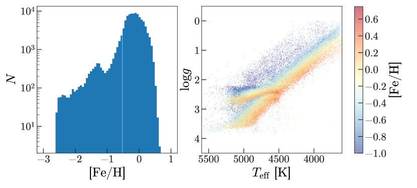
Figure 2: Left panel: Number of stars in bins of iron abundance, $[\textrm{Fe}/\textrm{H}]$, that pass the quality cuts described in Section 2. Right panel: Distribution of stars in our sample in stellar parameters log-surface-gravity, $\log g$, and effective temperature, $T_{\textrm{eff}}$, with points colored by the iron abundance.

Section 3 Methods

3.1 Orbit inference and velocity modeling

For every source in the sample of APOGEE stars defined in Section 2, we obtain a posterior sampling in binary-system parameter space, treating it as a single-lined (SB1) spectroscopic binary system with a single companion. This sampling is performed with The Joker (Price-Whelan et al. 2017) under a relatively uninformative prior pdf, and the resulting posterior samplings are used to discover and characterize individual binary-star systems and generate a catalog of companions. We now describe the assumptions and method used to generate samplings for individual systems:

no multiple companions

All radial-velocity variations of the primary star are induced by a single companion. This is motivated by the idea that triple star systems are usually hierarchical so that the period of the inner binary is typically much shorter than the orbital period of the outer body (e.g., Tokovinin 2018). At present, we ignore the possibility of higher-order multiple systems.

Kepler

All velocity variations of the primary are gravitational, and we therefore ignore the possibility of coherent intrinsic variation from, e.g., stellar oscillations.

SB1

All spectra are single-lined; that is, we assume that the secondary is significantly fainter and is thus undetected in the spectra. This assumption is motivated by the fact that we expect RGB stars to be substantially more luminous than their typical companion. However, there are known main-sequence double-lined binary stars in the APOGEE catalog (El-Badry et al. 2018), and an expected but unknown fraction of RGB–RGB binaries.

simple noise model

Measurements are unbiased and noise estimates are correct up to an unknown excess variance. All noise contributions result in Gaussian uncertainties on the individual radial-velocity measurements.

The Joker is a custom-built Monte Carlo sampler designed to produce independent posterior samples in Keplerian orbital parameters, given radial-velocity measurements under the assumptions listed above. Our parametrization of the orbital elements is similar to the notation in Murray & Correia (2010): The radial velocity $v$ at time $t$ is given by

$$v(t;\boldsymbol{\theta})=v_{0}+K\,[\cos\left(\omega+f(t;e,P,M_{0},t_{0})\right)+e\,\cos\omega]$$ (1)

where $\boldsymbol{\theta}=(P,e,M_{0},\omega,K,v_{0})$—period, eccentricity, mean anomaly at a reference time $t_{0}$, argument of pericenter, velocity semi-amplitude, barycentric velocity—and the true anomaly, $f$, is a function of time and the specified parameters (see Section 2 of Price-Whelan et al. 2017 or Equation 63 in Murray & Correia 2010). In addition to the orbital parameters listed above, The Joker can also generate samples in an “excess variance” parameter, $s^{2}$, that is added to the per-visit measurement variances. This parameter allows us to test whether the visit RV uncertainties are underestimated For upper RGB stars the inferred excess variance will be a combination of extra systematic uncertainty and true astrophysical surface jitter (e.g., Hekker et al. (2008)).

The Joker was designed for the extremely multi-modal pdf’s expected when the number of radial-velocity measurements of a source is small, or the data are sparse (in phase-coverage) or noisy. While other Markov Chain Monte Carlo (MCMC) methods have difficulty producing independent samples with such data, The Joker succeeds by brute force: After generating an initial (very large) library of prior samples from an assumed prior pdf (see below), the (typically multi-modal) likelihood is evaluated at each sample and used to rejection sample. In practice, given a number of requested samples for each star, the sampling proceeds iteratively: since it is easier to accept samples when the data is sparse or noisy, far more prior sample draws (and thus likelihood evaluations) must occur under very constraining data.

3.2 Individual-system posterior samplings

Here we describe the specifics of generating posterior samplings for all of the APOGEE targets in our parent sample. We execute the full procedure twice for different goals (as described in Section 5), and only here outline the key steps in the pipeline.

For all 96,231 APOGEE stars with $\geq 3$ good visits (see Section 2), we use The Joker to generate posterior samplings for each star under the assumptions listed above (see Section 3.1). We start by generating a library of 536,870,912 prior samples generated under a prior similar to that defined in Price-Whelan et al. (2017):

• uniform or isotropic in angle parameters,

• uniform in log-period over the domain $[1,32768]~{}\textrm{day}$,

• a beta distribution over eccentricity (using parameters from Kipping 2013).

For the excess variance parameter, $s^{2}$, we use a Gaussian over the transformed parameter $y=\ln s^{2}$ with the mean and standard deviation $(\mu_{y},\sigma_{y})$ indicated where the runs are described (see Section 5). The reference time for each star is set to the first visit epoch; $M_{0}$ then becomes the mean anomaly at the first visit observation. Table 1 contains descriptions of all parameters and priors used.

name	prior	description
$P$	$\ln P\sim\mathcal{U}(1,32768)~{}\textrm{day}$	period
$e$	$e\sim\textrm{Beta}(0.867,3.03)$	eccentricity
$t_{0}$	fixed	reference time
$M_{0}$	$M_{0}\sim\mathcal{U}(0,2\pi)~{}\textrm{rad}$	mean anomaly at reference time
$\omega$	$\omega\sim\mathcal{U}(0,2\pi)~{}\textrm{rad}$	argument of pericenter
$s^{2}$	$\ln s^{2}\sim\mathcal{N}(\mu_{y},\sigma_{y}^{2})$	extra variance added to each visit variance
$K$	$\mathcal{N}(0,\sigma_{v}^{2})~{}\mathrm{km}~{}\mathrm{s}^{-1}$	velocity semi-amplitude
$v_{0}$	$\mathcal{N}(0,\sigma_{v}^{2})~{}\mathrm{km}~{}\mathrm{s}^{-1}$	system barycentric velocity

Table 1: Summary and description of parameters. $\textrm{Beta}(a,b)$ is the beta distribution with shape parameters $(a,b)$, $\mathcal{U}(a,b)$ the uniform distribution over the domain $(a,b)$, and $\mathcal{N}(\mu,\sigma^{2})$ is the normal distribution with mean $\mu$ and variance $\sigma^{2}$. For the systemic velocity and semi-amplitude, $(v_{0},K)$, we use a broad Gaussian prior that is formally inconsistent between The Joker and follow-up MCMC sampling (see Section 3.2.1): in The Joker we assume Gaussian priors with $\sigma_{v}$ much larger than the measurement uncertainty so they can be neglected ($\sigma_{v}\approx\infty$), whereas when running MCMC we fix $\sigma_{v}=10^{3}~{}\mathrm{km}~{}\mathrm{s}^{-1}$.

We request 256 posterior samples for each source. Depending on the data quality and phase coverage of the visits, The Joker will require different numbers of prior samples in order to rejection-sample down to the requested number of posterior samples: For few-epoch or noisy RV data, many prior samples will pass the rejection step, whereas for very precise or many-epoch RV data, The Joker may need to process the full library of prior samples. We therefore generate the posterior samples using an iterative procedure that adaptively predicts how many prior samples to test for each star. For sources with very constraining data, The Joker may return fewer than the requested number of samples (as few as one sample). When this occurs, we continue sampling either using standard MCMC, or by increasing the size of the prior cache and continuing rejection sampling with The Joker.

3.2.1 “Needs MCMC”: Following up The Joker with MCMC

If just one posterior sample is returned after exhausting the full library of prior samples, or if multiple (but fewer than 256) are returned that all lie within a single mode of the posterior pdf, the posterior pdf over orbital parameters is treated as effectively unimodal: these stars are flagged “needs MCMC.” In this case, we use the location of the returned sample (if only one is returned), or a randomly chosen sample from those returned (if multiple samples are returned within one mode) to generate a small Gaussian ball of initial conditions and use standard MCMC to continue sampling until we obtain 256 samples.

In detail, we use an ensemble MCMC sampling algorithm (Goodman & Weare 2010) implemented in Python (emcee; Foreman-Mackey et al. 2013) to perform the samplings. We transform the standard Keplerian orbital parameters to a safer parametrization, $(\ln P,\sqrt{K}\,\cos M_{0},\sqrt{K}\,\sin M_{0},\sqrt{e}\,\cos\omega,\sqrt{e}\,\cos\omega,\ln s^{2},v_{0})$, for MCMC sampling. This reparametrization is safer and more efficient for sampling with emcee, which expects parameters to be components of a vector so that linear operations can be applied (see, e.g., Hogg & Foreman-Mackey 2017); the angle variables $(\omega,M_{0})$ don’t meet this requirement in the standard parametrization. We use the same prior pdf’s as in The Joker when running MCMC (see Table 1).

For each star that is flagged “needs MCMC,” we run emcee with 1024 walkers for 16384 steps, take the final walker positions, and downsample at random until we have 256 samples. We compute the Gelman–Rubin convergence statistic, $\hat{R}_{j}$, (Gelman & Rubin 1992) for each parameter $j$ and include these values in the catalogs below when standard MCMC is run. We also provide a binary flag, “converged,” for each sampling continued with MCMC that is set to true if:

$$\underset{j}{\textrm{mean}}\left(\hat{R}_{j}\right)<1.1\quad.$$ (2)

3.2.2 “Needs more prior samples”: Extending The Joker sampling

If more than one posterior sample is returned after exhausting the full library of prior samples, and the samples lie in multiple modes of the posterior pdf, the only way to proceed is to generate more prior samples and continue running The Joker: these stars are flagged “needs more prior samples.” In this case, we generate another equal-sized library of prior samples (a total of $2\times 536,870,912$ samples) and re-do the rejection sampling. We note that because of the way the rejection sampling step is done, this is not equivalent to concatenating the results from a second, independent run of The Joker: the log-likelihood values for all of the prior samples must be used. If at the end of this second run the target still has fewer than 256 samples, the sampling is flagged as “incomplete.”

3.3 Null comparison sample

We construct a comparison sample of simulated data with no RV variability to assess our false-positive rates in the selections below (see Section 5). We randomly pick 16,384 stars from the parent sample used in this work and replace the visit velocity measurements with simulated data. For each star $n$, we randomly sample an excess variance parameter value from the prior, $s_{n}$. For each visit $k$, we then sample a new velocity $v_{nk}$ by drawing from a Gaussian with mean equal to the mean of the real data visit velocities, $\bar{v}_{n}$, and variance equal to the sum of the visit variance (uncertainty), $\sigma_{nk}$, and the excess variance,

$$v_{nk}\sim\mathcal{N}(\bar{v}_{n},\sigma_{nk}^{2}+s_{n}^{2})\quad.$$ (3)

When we save the comparison data, we only store the visit uncertainty and “forget” the fact that the simulated data is generated with excess variance (to be inferrred with The Joker).

Section 4 Experiment: infer the excess variance distribution

With posterior samplings for all APOGEE DR14 systems in hand, and as an initial use of the per-source posterior samplings, we use a hierarchical Bayesian model to infer the parameters of the (assumed Gaussian) prior over the log-excess-variance parameter, $(\mu_{y},\sigma_{y})$ (see Table 1). This inference serves as a test-case for future work, where we intend to use the independent posterior samplings to construct a hierarchical inference over companion population properties. This is also a test of the visit velocity uncertainties reported in the APOGEE data products: If the catalog uncertainties are significantly underestimated, we expect the inferred log-excess-variance distribution parameters to tend towards larger values.

In detail, we maximize the marginal likelihood of the population-level parameters $(\mu_{y},\sigma_{y})$. We compute this marginal likelihood using the per-object posterior samples re-weighted by the ratio of the value of the hyperprior evaluated at a given, new set of parameters $(\mu_{y},\sigma_{y})$ over the value of the default prior at the previously assumed values, $(\mu_{y,0},\sigma_{y,0})$ (see above). This trick has been used in other hierarchical inferences as a way to marginalize over the per-object parameters to infer population-level parameters (Hogg et al. 2010; Foreman-Mackey et al. 2014); we describe how to compute the marginal likelihood in detail in Appendix A.

We execute a full run of The Joker on all 96,231 APOGEE stars in our parent sample using initial values for the excess variance distribution parameters chosen so that $\sqrt{e^{\mu_{y,0}}}\approx 200~{}\mathrm{m}~{}\mathrm{s}^{-1}$: $(\mu_{y,0},\sigma_{y,0})=(10.6,3)$ in units of $\mathrm{m}~{}\mathrm{s}^{-1}$. This run took approximately 300 hours on a compute cluster with 448 cores, with the time dominated by sources with many ($\gtrsim 10$) visits. For this initial run, we do not follow up on stars that return $<$256 samples.

We use 1,825 stars with $>10$ visits and $\log g>2$ (to avoid upper RGB stars that have large intrinsic jitter) and maximize the above likelihood to determine better hyperparameters for the log-excess-variance parameter distribution. Figure 3 shows the distribution corresponding to the maximum-likelihood hyperparameters, $\alpha^{*}=(\mu_{y}^{*},\sigma_{y}^{*})=(9.50,1.64)$. These values are consistent with the estimated systematic floor of the visit velocity uncertainties of $\approx 100$–$200~{}\mathrm{m}~{}\mathrm{s}^{-1}$ estimated from stars observed multiple times and on multiple plates (Nidever et al. 2015).

However, there are a number of caveats to keep in mind about this estimate of the excess variance distribution. First, we do not remove triple or other multiple systems: For any individual system, the radial velocity variations induced by other massive bodies will lead to larger preferred values for the excess variance parameter. We do not expect there to be a large number of triple systems in our sample, but this is still an important consideration for future efforts. Second, we are sensitive to outliers and very non-Gaussian systematic error distributions. We later assess the non-Gaussianity of the visit velocity uncertainties by looking at the visit velocity residuals away from the orbit samples produced by The Joker using the updated excess variance distribution (see Section 7.2).

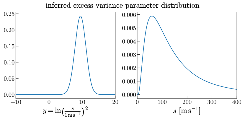
Figure 3: Inferred prior over excess variance parameter ($y=\ln s^{2}$) using posterior samples for 1,825 lower-RGB stars with $>10$ visits. Left and right panels show the distribution corresponding to the maximum-likelihood parameters $(\mu_{y},\sigma_{y})=(9.50,1.64)$ in log and linear, respectively.

Section 5 Companion catalogs

Using the most likely hyperparameters derived from the initial posterior samplings (see Section 4), we update and fix the excess variance prior distribution parameters—$(\mu_{y},\sigma_{y})=(9.50,1.64)$, in units of $\textrm{m}~{}\textrm{s}^{-1}$—and re-run The Joker on the parent sample of APOGEE DR14 stars. This approach of estimating a prior pdf from the data and then fixing the parameters is typically referred to as “empirical Bayes”; in this case, it is an approximation to doing a hierarchical inference of the individual system orbital parameters and the excess variance distribution hyperparameters simultaneously.

From this run, 91,096 stars completed and successfully returned 256 samples using The Joker alone. The remaining 5,135 stars did not return 256 samples: 4,744 were flagged as needs more prior samples, 391 as needs MCMC. We then proceed to generate 256 samples for these two subsets using the methodology explained above (see Section 3.2). The full catalog of posterior samples for all APOGEE stars in our parent sample is available online.

We also run on the null comparison sample (see Section 3.3) with the same parameters. From the comparison sample run, 13 “stars” are flagged as needs MCMC, and 1023 are flagged as “needs more prior samples”; For these comparison sample stars, we don’t continue sampling with The Joker or MCMC and only use the ($<$256) posterior samples returned from the The Joker.

5.1 Stars with companions

We do not expect a sharp transition in inferred orbital parameters between stars with and without companions: There is a continuum of companion properties. For example, the companions can be low mass, or at long periods, or at high inclination, all of which will make the velocity semi-amplitude, $K$, small for a given system. Therefore, there is no simple cut on radial velocity data alone that would select a complete sample of stars with companions. It is nevertheless possible to define a cut that selects stars with high-confidence companions.

We select a sample of stars that confidently have companions using percentiles computed from the log of the posterior samples in the velocity semi-amplitude parameter, $\ln K$. Figure 4, shows the distribution of 1st percentiles of $\ln K$ computed for all stars with posterior samplings from The Joker (filled, blue histogram), along with the same for posterior samplings for the null comparison sample (solid, dark line). To select stars with companions, we use a cut in the 1st percentile of the $\ln K$ samples such that $1\%$ of the comparison sample is selected, i.e. our estimated false positive rate is $\approx 1\%$. We use a threshold of $\ln K=-0.2$ to meet this constraint (vertical, dashed line in Figure 4); 4,898 stars pass this cut. For brevity below, we refer to this sample as the “high-$K$” stars, and the complimentary sample as the “low-$K$” stars.

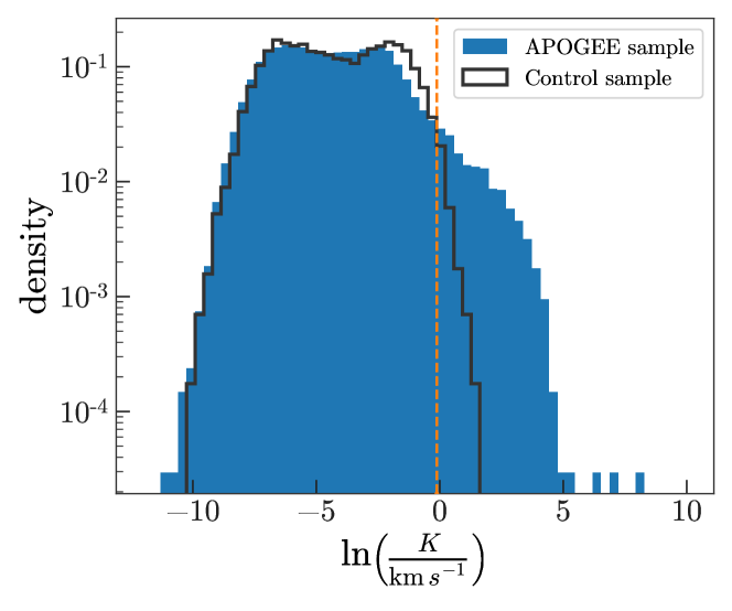
Figure 4: Distribution of 1st percentiles in $\ln K$ (in units of $\mathrm{km}~{}\mathrm{s}^{-1}$) for the parent APOGEE sample (blue, filled) and for the comparison sample (solid, dark line). The vertical line (dashed, orange) indicates our adopted cut to select high-$K$ stars that likely have companions at $\ln K=-0.2$; $1\%$ of the comparison sample falls above this cut.

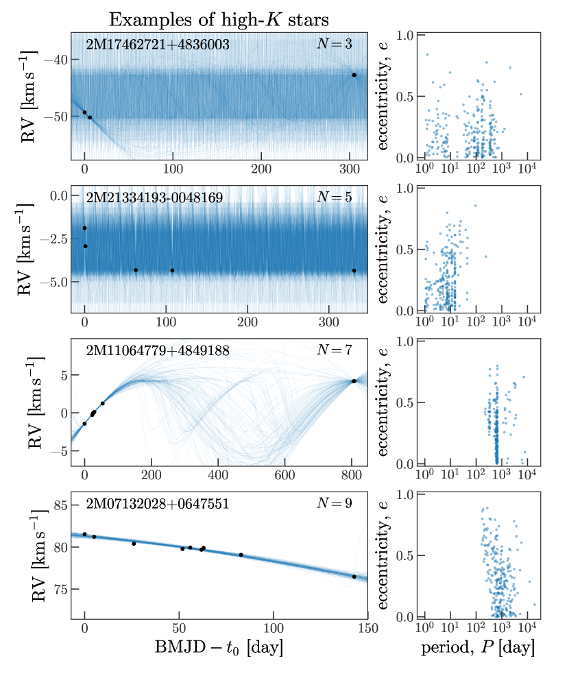
Figure 8: Examples of stars in our high-$K$ sample, i.e. stars that likely have companions (see Section 5.1), with different numbers of visits. Left panels show the data (black markers, error bars are the visit velocity uncertainties) with 128 random orbits from the 256 posterior samples under-plotted (lines, blue); The APOGEE_ID of each target and the number of visits that pass our quality cuts, $N$, are indicated on each panel. Right panels show the 256 posterior samples visualized in period–eccentricity space. In most cases, despite confidently having companions based on the RV amplitude, the permitted orbit fits are highly multimodal.

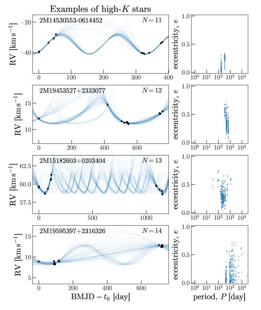
Figure 9: Continuation of Figure 8.

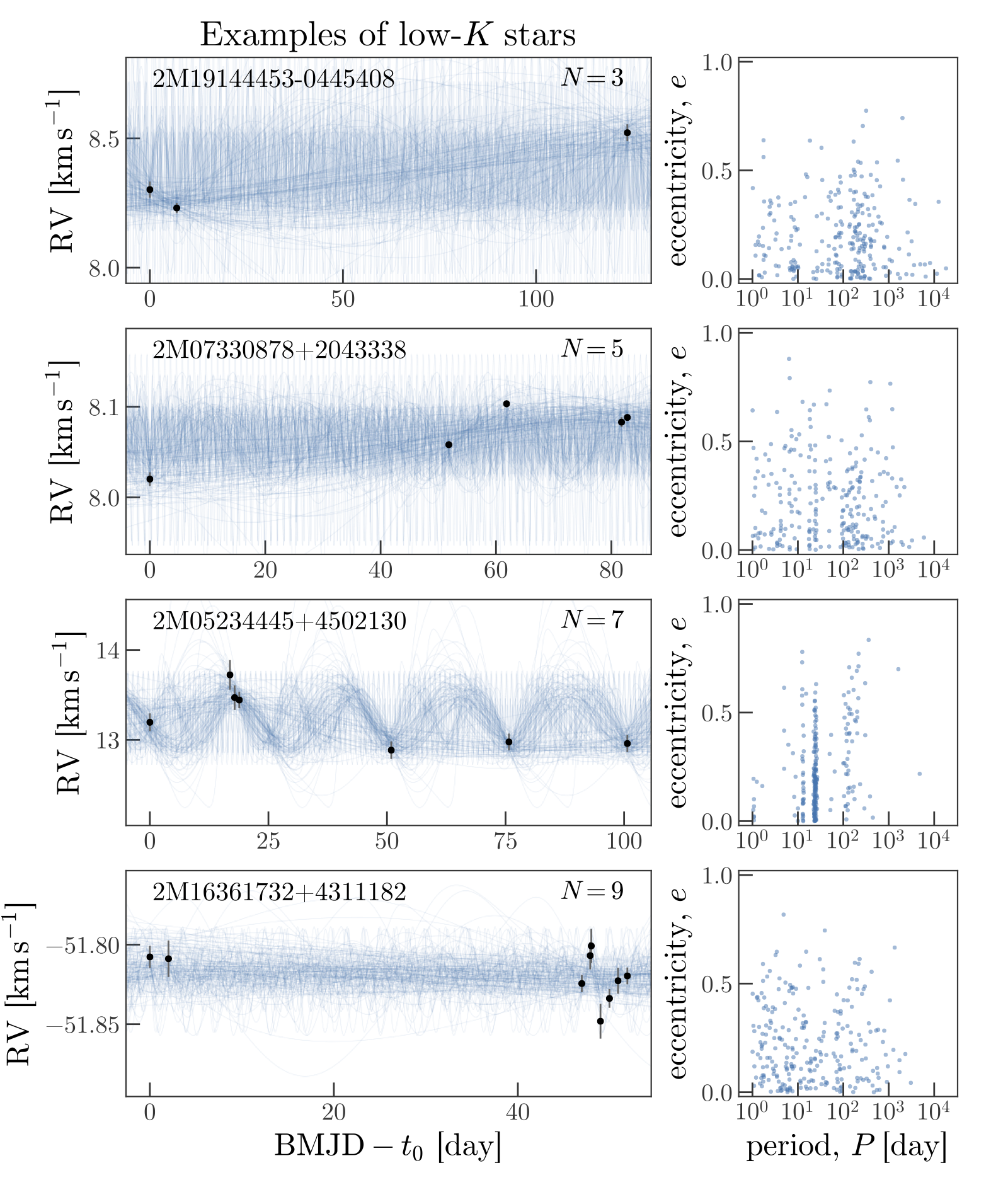
Figure 10: Same as Figure 8, but for stars in the low-$K$ sample, i.e. stars that have undetected or no companions.

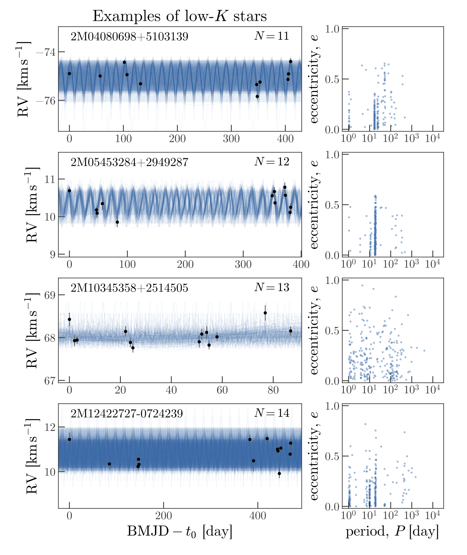
Figure 11: Continuation of Figure 10.

Table 2 contains a list of all stars in the parent sample and the value of the 1st percentile over the $\ln K$ samples for each star. Figures 8 and 9 show eight examples of high-$K$ stars, i.e. stars that likely have companions, with different numbers of visits, $N$, indicated on the panels. Figures 10 and 11 shows the same for eight low-$K$ stars, i.e. stars that either have no companions, low-mass companions, or companions at long periods or high inclination. The majority of the stars in the high-$K$ sample have poorly constrained orbital parameters because the posterior pdf’s are very multimodal. The high-$K$ sample selected from Table 2 includes all stars in the catalogs described in the next two subsections, however the following two catalogs are mutually exclusive.

5.2 Companions with uniquely-determined orbits

Starting from the high-$K$ sample, we select stars that have posterior period samples that fall within a single mode. We define a period resolution for each star $\Delta=\left[4\,P_{\textrm{min}}^{2}/(2\pi\,T)\right]$, where $P_{\textrm{min}}$ is the minimum period sample value, and $T$ is the epoch span of the data for that star. We consider a sampling to be unimodal when

$$P_{\textrm{max}}-P_{\textrm{min}}<\Delta$$ (4)

(see Section 2 of Price-Whelan et al. 2017); 320 stars pass this cut. Unlike the multi-modal stars, the posterior pdf’s for these stars can be approximated using point-estimates and standard deviations of their respective samplings. We report maximum a posteriori (MAP) sample values for the orbital parameters, along with other computed quantities for all 320 stars in this high-$K$, unimodal sample. For stars with measured primary masses, $M_{1}$, from other work (Ness et al. 2015), we compute the minimum companion mass, $M_{2,\textrm{min}}$ and include both masses in this catalog. We additionally join with the APOGEE DR14 allStar catalog and provide all columns from this catalog for convenience. Table 3 contains descriptions and units for all columns in the high-$K$, unimodal sample catalog, available online.

We have also visually inspected the inferred orbits for all systems in this sample and have flagged systems with questionable or invalid fits. The value of the flag is: 0, when the orbits look reasonable, 1, when the orbits look reasonable but the value of the inferred excess variance is large, and 2, when the orbits are clearly poor fits. Many of the stars flagged as “2” look like they may be triple systems, as they tend to have radial velocity variations over two distinct timescales that are never well-fit by a single Keplerian orbit. The stars flagged as “1” tend to be either upper RGB stars, where astrophysical surface jitter can lead to RV modulations, or SB2 systems, where absorption lines from the secondary confuse the RV pipeline and lead to strange RV signals. This flag is included in the catalog (Table 3) as the column clean_flag; To select a clean sample of companions that have been successfully vetted by-eye, select only stars with clean_flag == 0.

5.3 Companions with highly constrained orbits

A subset of the high-$K$ sample (Section 5.1) have multimodal posterior distributions over orbital parameters that are limited to a few qualitatively different solutions. For these stars, one or a few more RV measurements would likely lead to uniquely-determined orbital parameters, making these stars prime candidates for follow-up efforts. As examples of such cases, we include an additional catalog of systems that have effectively bimodal posterior samplings in orbital period. We identify these systems using $k$-means clustering (Lloyd 1982) of the posterior samples in period. In detail, for all stars in the high-$K$ sample, we compute $\ln P$ for all period samples, then use $k$-means clustering with $k=2$ as implemented in the scikit-learn package (Pedregosa et al. 2011) to identify two clusters of samples. We initialize the cluster positions at either end of the range of possible periods. For each cluster, we then ask whether the samples assigned to that cluster are unimodal (Equation 4). If the samples in each respective cluster are unimodal, we call the sampling “bimodal”; 106 systems are identified as bimodal.

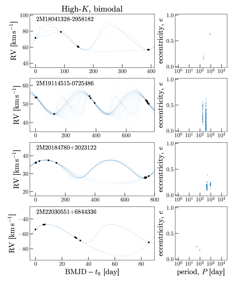
Figure 13: Randomly-selected examples of high-$K$ stars with bimodal posterior samplings. Same as Figure 12, but for bimodal posterior samplings.

Figure 13 shows a few examples of systems that meet this criterion. In many of these cases, there are certain times at which a future observation would be far more informative. Visually, those times correspond to regions of time when the predicted RVs have large variance based on the posterior samples at hand. For example, in the bottom left panel of Figure 13, an observation at $t=60$ would rule out one of the two possible classes of orbits.

Table 4 contains a list of all APOGEE targets with bimodal samplings identified in this way. The table contains two rows for each source, with the period, eccentricity, and velocity semi-amplitude values from the MAP sample from each period mode. When available, this table also includes an estimate of the primary mass, $M_{1}$, from Ness et al. (2015) and an estimate of the minimum companion mass, $M_{2,\textrm{min}}$ for each mode.

We again visually inspect all systems in this sample and assign a flag based on the apparent quality of the inferred orbits (see Section 5.2). Again, to select a clean sample of companions from this catalog that have been successfully vetted by-eye, select only stars with clean_flag == 0.

Section 6 Results

Here we highlight a few interesting results from visualizing the properties of companions in the unimodal and bimodal samples defined above (see Sections 5.2 and 5.3). In all figures below, we only plot companions with inferred orbits that pass our visual inspection (clean_flag == 0).

6.1 Systems with unimodal and bimodal posterior samplings

Figure 5 shows the companion and stellar properties of the unimodal and bimodal samples: upper left panel shows inferred period and eccentricity of the binary orbit, lower left panel shows inferred period and surface gravity of the primary star, lower right panel shows the primary star stellar parameters.

The period-eccentricity plot (upper left panel in Figure 5) shows a clear signature of tidal circularization: Such plots for main sequence stars typically show a more distinct circularization period, below which the majority of stars have eccentricities close to zero. Here, we see that close to $P\approx 10~{}\textrm{day}$ the majority of companion orbits appear to be circular, but between 10–100 days there appears to be a gradual decrease in eccentricity rather than a sharp transition. This is likely because the primary stars in this sample have a large range in surface gravities and therefore a large range in stellar radii (see lower right panel).

In the lower left panel of Figure 5, the diagonal (thick) line shows the orbital period of a hypothetical massless companion at the surface of a $1.35~{}\mathrm{M}_{\odot}$ primary star (the median of our sample with measured masses) with the given surface gravity. The vertical line in this panel shows the same for a $1.35~{}\mathrm{M}_{\odot}$ primary with $\log g=0$, i.e. the orbital period at the surface of such a star close to the tip of the RGB. The horizontal line in this panel shows the approximate upper bound of the red clump, above which most stars should be fully convective. Interestingly, there is a dearth of short-period systems for stars above the red clump ($\log g\lesssim 2.3$) in the triangle defined by the three qualitative lines, suggestive of possible companion engulfment as the primary star envelope encases the companion.

The lower right panel of Figure 5 shows the stellar parameters of all primary stars in the unimodal and bimodal samples. Relative to Figure 2, upper RGB stars appear to be under-represented in these companion catalogs, another tentative signature of engulfment or depletion of companions on shorter-period orbits.

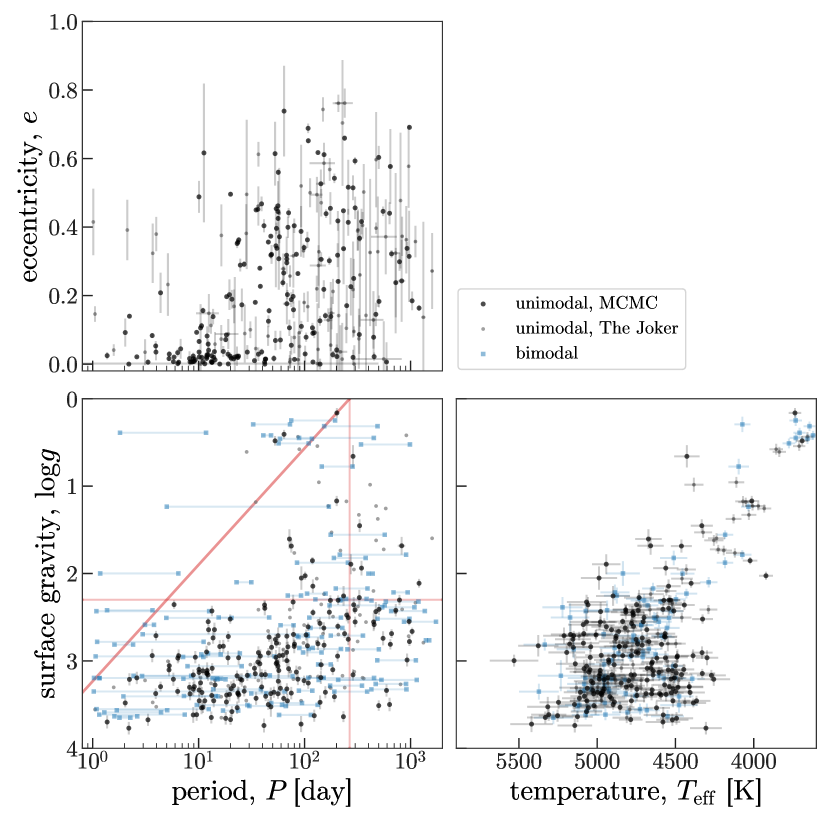
Figure 5: Top: Inferred orbital period and eccentricity for all systems with unimodal and bimodal posterior samplings from The Joker. Bottom left: Inferred orbital period and primary star surface gravity, $\log g$. Diagonal line indicates the orbital period of a hypothetical massless companion at the surface of a $1.35~{}\mathrm{M}_{\odot}$ primary star with the given $\log g$, vertical line shows the same for $\log g=0$, and horizontal line shows the rough upper boundary of the red clump. Bottom Right: Stellar parameters for all primary stars in the unimodal and bimodal samples.

6.2 Companion masses and mass ratios

Most of the companions we find have minimum masses $M_{2,\textrm{min}}<1~{}\mathrm{M}_{\odot}$. Figure 6, left panel shows primary and companion mass estimates for systems with unimodal (circle markers) and bimodal (square markes, blue lines) period samplings for the subset of 69/320 unimodal and 25/106 bimodal systems with primary mass estimates, again using primary masses from Ness et al. (2015). Upper dashed line shows the $M_{2,\textrm{min}}=M_{1}$ curve, and lower dashed line shows the Hydrogen-burning limit, $M_{2,\textrm{min}}=0.08~{}\mathrm{M}_{\odot}$. For the systems with bimodal samplings, we compute the minimum companion mass for each period mode and connect these estimates with a line. Here we restrict to stars with $\log g>2$ to avoid upper RGB stars that may have surface oscillations that mimic RV modulations from companions.

Figure 6, right panel shows the ratio of the primary stellar radius to the projected separation of the two bodies, $R_{1}/(a\,\sin i)$, and the minimum mass ratio, $q_{\textrm{min}}=M_{2,\textrm{min}}/M_{1}$, for the same systems. Again, circle (black, grey) markers indicate systems from the unimodal sample, and square (blue) markers and lines connect the two estimates for systems with bimodal period samplings. Upper dashed line in this panel indicates the Roche radius, computed using an approximate functional form (Eggleton 1983)

$$\frac{R}{a}=\frac{0.49\,q^{-2/3}}{0.6\,q^{-2/3}+\ln\left(1+q^{-1/3}\right)}$$ (5)

where $q=M_{2}/M_{1}$. All of these systems are consistent with being detached binaries, with the exception of one notable system (discussed below).

In Figure 6, a few interesting systems are immediately obvious: From the left panel, two systems have bimodal period samplings in which both period modes put the minimum companion mass below the Hydrogen-burning limit (brown dwarf candidates), and two systems have $M_{2,\textrm{min}}>M_{1}$ (neutron star or black hole candidates). In the right panel, one system appears right on the limit of being an interacting binary ($q_{\textrm{min}}\approx 0.5$), but has no significant UV flux (GALEX DR5; Bianchi et al. 2011). These systems are prime candidates for spectroscopic follow-up.

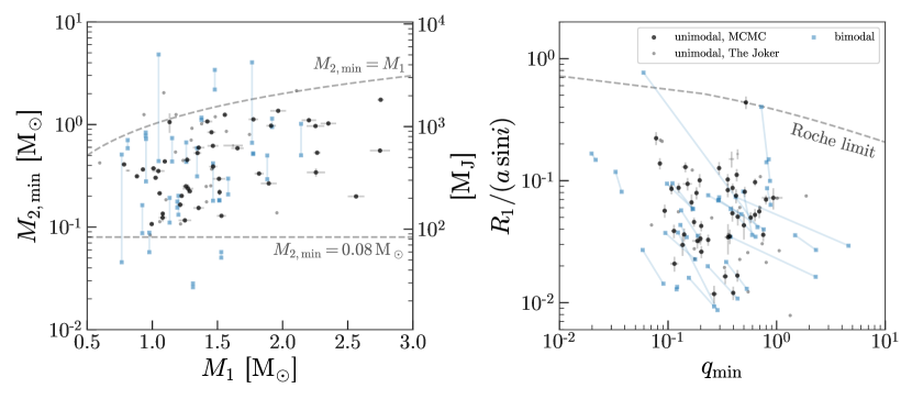
Figure 6: Left panel: Estimated minimum companion mass and primary mass for a subset of the systems in the high-$K$, unimodal converged sample (31 systems; black circles), unimodal unconverged sample (38 systems; grey circles), and bimodal sample (25 systems; blue squares and lines) with $\log g>2$ and previously measured primary masses (Ness et al. 2015). Lines connecting markers (blue) show estimates from each period mode for each system with bimodal period samplings. Upper, dashed line shows the equal-mass curve, and lower dashed line shows the Hydrogen-burning limit. Right panel: Ratio of primary stellar radius, $R_{1}$, to projected separation of the two bodies, $a\,\sin i$, and minimum mass ratio, $q_{\textrm{min}}$, for the same systems and markers in left panel.

Section 7 Discussion

7.1 Impossible companions and the upper RGB

Paradoxically, there appear to exist short period ($\lesssim 100~{}\textrm{day}$) companions at low surface gravities ($\log g\lesssim 1$), obvious in the lower-left panel of Figure 5: These companions would orbit within the surface of their primary stars. Each of these systems appears fine from the APOGEE data quality flags, but could nonetheless have incorrect stellar parameters. As a test, we would ideally be able to compare the spectroscopic stellar parameters to an independent determination from, e.g., asteroseismology. Unfortunately, none of these short-period, low-$\log g$ stars in the unimodal or bimodal samples appear in the APOKASC (Serenelli et al. 2017) catalog, which provides asteroseismic stellar parameters for a few hundred APOGEE dwarf and giant stars. We therefore instead cross-match all high-$K$ stars with $\log g<1$ and $99\%$ of their period samples below $100~{}\textrm{day}$ to the APOKASC catalog: One star appears in both samples 2M19024490+4419523. In APOGEE DR14, this star has $\log g=0.57$, but asteroseismic $\log g>4$ (e.g., HUBER_LOGG), consistent with being an M dwarf. Many of these systems could therefore be low-mass dwarf stars with incorrect stellar parameters in APOGEE DR14.

Another possibility is that The Joker interprets semi-coherent surface oscillations (from asteroseismic modes) with sparse time coverage as orbital RV variations (see, e.g., Hekker et al. 2008). However, for RGB stars with $\log g<1$, these modes would likely have frequencies between $\nu_{\textrm{max}}\approx 0.5$–$5~{}\mu\textrm{Hz}$ (Garcia & Stello 2018), corresponding to periods between $P\approx 20$–$2~{}\textrm{day}$ and amplitudes between $\approx 20$–$200~{}\textrm{m}~{}\textrm{s}^{-1}$ (Huber et al. 2011; Huber 2017). Except for the lowest $\log g$ stars, these amplitudes wouldn’t pass our cut on $K$ (Section 5.1).

These systems would need precise, long-term photometric follow-up to obtain asteroseismic parameters to confirm or explain their existence.

7.2 Assumptions

It is important to keep in mind that the companion catalogs and results presented in this Article depend on the assumptions laid out in Section 3.1. We have only considered radial velocity modulations from a single massive companion—no multiple companions; This is a fundamental limitation of our search and methodology. However, stars with multiple companions will likely be included in our companion catalog anyway, only with two-body orbital solutions that either don’t fit the data well or pick out the shortest period orbit.

Related to the above, we assume that all RV variations are gravitational—Kepler. We see tentative evidence for surface oscillations at the upper giant branch (see Figure 5, lower left), which we presently treat as excess variance or intrinsic jitter. Further observations are needed to determine whether these “systems” have incorrect stellar parameters, or indeed show surface oscillations related to asteroseismic modes.

We assume that one star in each two-body system overwhelmingly dominates the luminosity and therefore spectrum of each system—SB1. As seen in Figure 6, there are some companions with minimum masses comparable to or consistent with being larger than the masses of the observed star. These systems are either (a) nearly edge-on MS–RGB binaries (i.e. consistent with our assumption), (b) SB2 systems where the APOGEE pipeline failed to flag the source as having broad lines or a bad fit, or (c) RGB–stellar remnant systems with a black hole or neutron star companion. A subset of these systems that look like they fall in category (c) are being followed-up to obtain further RV measurements to test whether any companions are black holes. However, The Joker can and should be extended to support sampling for SB2 systems with just one additional parameter (typically the mass ratio, or ratio of velocity semi-amplitudes).

Finally, we have assumed that the visit velocity error distribution is Gaussian, and that the visit velocity uncertainties could be under-estimated—simple noise model. We can test this assumption using posterior samples from The Joker by computing the residuals away from our best-fit two-body orbital solutions. We find that the normalized residuals appear to be very close to Gaussian over a large dynamic range of normalized residual values, indicating that this assumption may be sufficient. Figure 7 shows the distribution of normalized residuals, $R_{nk}$, for each visit: the $k$ visit velocities for each $n$ star, $v_{nk}$, minus the predicted radial velocity from the best-fitting sample returned by The Joker, $\hat{v}^{*}_{nk}$, normalized by the excess-variance-included uncertainty, $\sigma_{nk}^{*}=\sqrt{\sigma_{nk}^{2}+\hat{s}_{n}^{2}}$, where $\hat{s}_{n}$ is computed from the excess-variance parameter of the best-fitting sample:

$$R_{nk}=\frac{v_{nk}-\hat{v}^{*}_{nk}}{\sqrt{\sigma_{nk}^{2}+\hat{s}_{n}^{2}}}\quad.$$ (6)

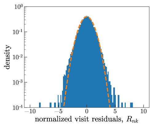
Figure 7: Histogram shows the distribution of normalized visit residuals (see Equation 6) for all 397,559 used in the final run of The Joker (i.e. with updated excess variance distribution parameters inferred in Section 4). The orange curve shows that expected for Gaussian uncertainties. The distribution appears mostly Gaussian over a large range of residual values, with slightly more populated tails and evidence of a few catastrophic outliers.

7.3 Comparison to other APOGEE companion catalogs

There are at least two other recent catalogs of stellar systems and companions based on APOGEE data.

One of these studies focused on decomposing spectra of MS stars into mixtures of stellar spectra (El-Badry et al. 2018). Conceptually, this method works because (a) for two unequal-mass stars, unexpected absorption lines will appear superimposed on the brighter star’s spectrum, and (b) for close to equal-mass stars, the line depths and ratios will not be well-matched by a single stellar model. Using this technique, they identified thousands of candidate MS binaries and trinaries, but did not consider giant stars ($\log g>4$). This sample is therefore complimentary to and non-overlapping with the catalog presented in this work.

The other recent catalog searched for stellar and substellar companions to all stars in APOGEE DR12 (including the RGB) that passed a series of quality cuts, and had $\geq 8$ visits (Troup et al. 2016). For each star in the sample, orbits were fit to the visit RVs using a multi-step orbit-fitting procedure: it starts by identifying significant periods and a few harmonics of those periods, then fits a Keplerian orbit at each of these harmonics using least-squares fitting (De Lee et al. 2013) with a modified $\chi^{2}$ statistic that penalizes fits in which the phase coverage of the data is poor. This procedure is not guaranteed to provide a unique orbit solution.

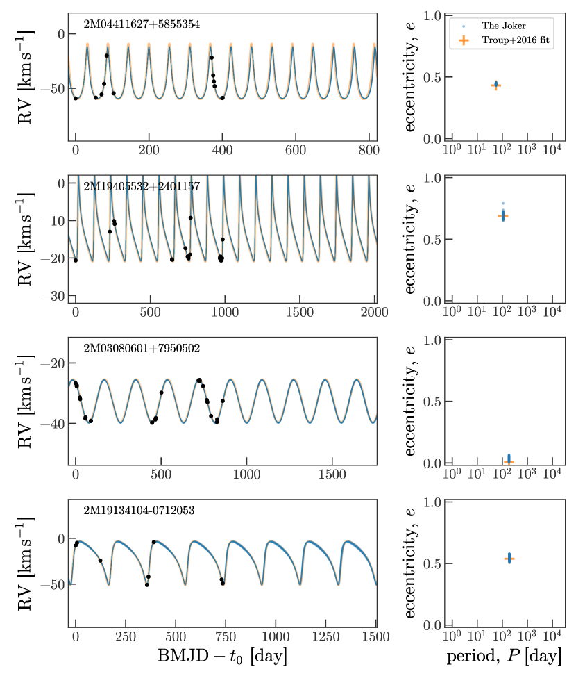
Figure 14: Four examples of stars that also appear in the Troup et al. (2016) companion catalog where our orbit samplings are unimodal, and agree well with the previous orbit fits. Left panels show the data from APOGEE DR14 (black markers), the orbit fit (orange, thick line; Troup et al. 2016), and 128 orbits computed from posterior samples generated in this work (blue, thinner lines). Right panels show the period and eccentricity of the orbit fit (orange, + marker; Troup et al. 2016) and the posterior samples from this work (blue markers).

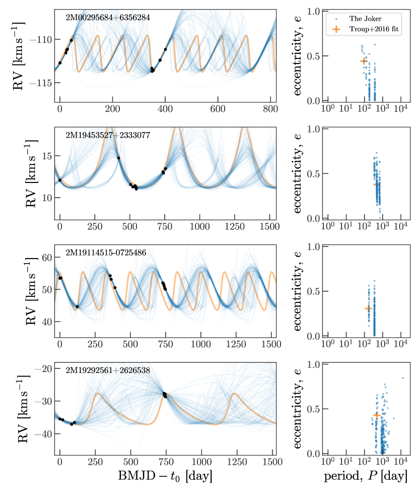
Figure 15: Same as Figure 14, but for four stars where we find a multi-modal posterior sampling. In this cases, the orbit fit from Troup et al. (2016) generally identify one of the possible period modes, but multiple orbit solutions are typically allowed.

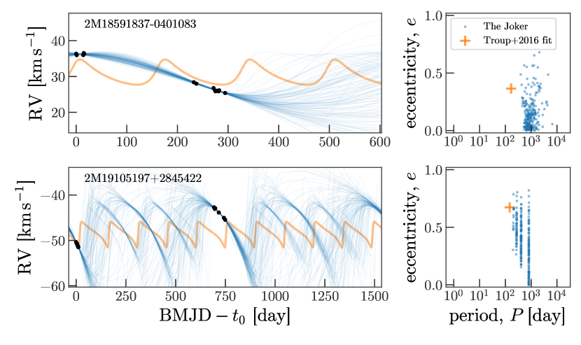
Figure 16: Same as Figure 14 and Figure 15, but for two stars in which no meaningful comparison can be made because the visit velocities changed significantly between DR12 and DR14.

Of the 382 companions released as a part of the Troup et al. (2016) search, only 188 of the host stars passed the stellar parameter and quality cuts used to define the parent sample in this work (see Section 2). We have looked at all of the overlapping stars to compare the previously derived companion orbital properties to the posterior samplings derived with The Joker. We find that the comparisons fall in three categories: (1) the parameters reported in Troup et al. (2016) agree with the posterior samplings, and the period distribution appears unimodal, (2) the parameters reported in Troup et al. (2016) identify one possible mode of a likely multi-modal posterior pdf over orbital parameters, and (3) the radial velocity data used in Troup et al. (2016) changed significantly between APOGEE DR12 and DR14, so no meaningful comparisons can be made; roughly 1/3 of the comparison sample falls into each class. Figure 14 shows a few representative cases in which the Troup et al. (2016) orbital parameters (orbit shown as orange line in left panels, parameters shown as orange + in right panels) is consistent with the orbit samples from The Joker. Figure 15 shows a few representative cases in which we find that the posterior pdf over orbital parameters is multimodal, and the Troup et al. (2016) orbit identifies one of these modes. For completeness, Figure 16 shows two instances in which the orbital parameters from Troup et al. (2016) no longer make sense, likely because the data changed between data releases.

7.4 Population inference

The main motivation for this work was to produce posterior samplings for all APOGEE DR14 stars to be used in a population inference. To use these samplings for population or hierarchical inference, the orbits of each individual system don’t have to be unimodal and thus all 96,231 samplings can be used in conjunction without well-determined orbital parameters for the majority of the stars. These samplings will be useful for constraining (through hierarchical inference) the period and eccentricity distributions of evolved stars, and the occurrence rates of companions to evolved stars to test for signatures of engulfment.

Section 8 Conclusions

We have selected a catalog of nearly 5,000 stellar systems with companions by making cuts on posterior beliefs about the amplitude of orbital radial velocity variations for often low-epoch, sparsely sampled radial velocity data. We provide posterior samplings over orbital parameters for all 96,231 in the parent sample of APOGEE DR14 systems used in this work, along with several sub-catalogs with better constrained orbital information:

• A catalog of 320 systems with unimodal posterior samplings, and therefore uniquely determined orbits, of which 225 are newly discovered binary star systems.

• A catalog of 106 systems with highly constrained posterior samplings that, in period, span two distinct period modes. For these systems, one or a few more radial velocity measurements would uniquely determine their orbits. 90 of these systems are newly discovered binary star systems.

• A catalog of 4,898 systems with radial velocity variations consistent with having a companion, but which need further radial velocity measurements to better constrain the orbital properties.

All companion catalogs described in this work (Section 5) are available online.

The source code for this project is open source and available from https://github.com/adrn/TwoFace under the MIT open source software license.

Appendix A Hierarchical inference of the excess variance parameter

For each $n$ of $N$ RGB stars in APOGEE, we obtain $M$ posterior samples over primary orbital parameters $\boldsymbol{\theta}=(P,e,\omega,M_{0},K,v_{0})$ and the excess-variance parameter, $y=\ln s^{2}$, using The Joker; For brevity in expressions below, we will use the vector

$$\boldsymbol{w}=(\boldsymbol{\theta},y)$$ (A1)

to represent the full set of parameters. To obtain this sampling, we use an interim (Gaussian) prior on the excess-variance parameter parametrized by a mean and standard deviation, i.e. $\alpha_{0}=(\mu_{y,0},\sigma_{y,0})$ as described above. For a given source, the posterior samples in the above parameters are drawn from the distribution

$$\boldsymbol{w}_{m}\sim p(\boldsymbol{w}_{m}\,|\,D,\boldsymbol{\alpha}_{0})$$ (A2)

where $D$ represents the data for a given object.

We want to compute the likelihood of all data from all $N$ stars, $\{D_{n}\}$, given a new set of hyperparameters $\boldsymbol{\alpha}$

$$p(\{D_{n}\}\,|\,\boldsymbol{\alpha})=\prod_{n}^{N}p(D_{n}\,|\,\boldsymbol{\alpha})$$ (A3)

where in the above, we have assumed that this likelihood is separable ( the data for each source are independent). The per-source marginal likelihood in the above expression is given by

$$p(D_{n}\,|\,\boldsymbol{\alpha}) =\int\mathrm{d}\boldsymbol{w}_{n}\,p(D_{n}\,|\,\boldsymbol{w}_{n})\,p(\boldsymbol{w}_{n}\,|\,\boldsymbol{\alpha})$$ (A4)

$$=\int\mathrm{d}\boldsymbol{w}_{n}\,p(D_{n}\,|\,\boldsymbol{w}_{n})\,p(\boldsymbol{w}_{n}\,|\,\boldsymbol{\alpha})\,\frac{p(\boldsymbol{w}_{n}\,|\,D_{n},\boldsymbol{\alpha}_{0})}{p(\boldsymbol{w}_{n}\,|\,D_{n},\boldsymbol{\alpha}_{0})}$$ (A5)

$$=p(D_{n}\,|\,\boldsymbol{\alpha}_{0})\,\int\mathrm{d}\boldsymbol{w}_{n}\,\frac{p(\boldsymbol{w}_{n}\,|\,\boldsymbol{\alpha})}{p(\boldsymbol{w}_{n}\,|\,\boldsymbol{\alpha}_{0})}\,p(\boldsymbol{w}_{n}\,|\,D_{n},\boldsymbol{\alpha}_{0})\quad.$$ (A6)

Using the Monte Carlo integration approximation, Equation A6 can be simplified to a sum over prior value ratios of the $M$ posterior samples in the log-excess-variance parameter for each $n$ star

$$\approx\frac{\mathcal{Z}_{n}}{M}\,\sum_{m}^{M}\frac{p(y_{nm}\,|\,\boldsymbol{\alpha})}{p(y_{nm}\,|\,\boldsymbol{\alpha}_{0})}$$ (A7)

where we have canceled the other priors (over $\boldsymbol{\theta}$), and all normalization constants appear in the constant scale factor $\mathcal{Z}_{n}$.

The above expresion gives the marginal likelihood of the velocity data for a single source given new hyperparameters $\boldsymbol{\alpha}$. The full marginal likelihood is then the product of these individual likelihoods

$$p(\{D_{n}\}\,|\,\alpha) \propto\prod_{n}^{N}\frac{1}{M}\,\sum_{m}^{M}\frac{p(y_{nm}\,|\,\alpha)}{p(y_{nm}\,|\,\alpha_{0})}\quad.$$ (A8)

In practice, we evaluate the log-marginal-likelihood

$$\ln p(\{D_{n}\}\,|\,\alpha) \propto\sum_{n}^{N}\left[\ln\left(\sum_{m}^{M}\frac{p(y_{nm}\,|\,\alpha)}{p(y_{nm}\,|\,\alpha_{0})}\right)-\ln M\right]$$ (A9)

$$\propto\sum_{n}^{N}\left[\underset{k}{\textrm{logsumexp}}\left[\ln{p(y_{nm}\,|\,\alpha)}-\ln{p(y_{nm}\,|\,\alpha_{0})}\right]-\ln M\right]$$ (A10)

where logsumexp (the log-sum-exp trick) provides a more stable estimate of the sum in Equation A9.

Appendix B Data products

Parent sample of APOGEE DR14 stars
APOGEE_ID	lnK_per_1
2M00000002+7417074	-2.028
2M00000068+5710233	-2.600
2M00000222+5625359	2.134
2M00000446+5854329	-7.199
…	…
(96,231 rows)

Table 2: This table contains APOGEE_ID’s for all 96,231 stars in the parent sample used in this work, for which we have posterior samplings in orbital parameters. The other column contains the 1st percentile computed over the $\ln K$ samples for each source, lnK_per_1: The “high-$K$” sample (see Section 5.1) is defined using this column, by selecting lnK_per_1 > 0.

High-$K$, unimodal systems
Column name	Unit / format	Description
APOGEE_ID		identifier used by APOGEE
P	$\mathrm{d}$	$P$, period
P_err	$\mathrm{d}$
M0	$\mathrm{rad}$	$M_{0}$, phase at reference epoch
M0_err	$\mathrm{rad}$
e		$e$, eccentricity
e_err
omega	$\mathrm{rad}$	$\omega$, argument of pericenter
omega_err	$\mathrm{rad}$
jitter	$\mathrm{km\,s^{-1}}$	$s$, excess variance parameter
jitter_err	$\mathrm{km\,s^{-1}}$
K	$\mathrm{km\,s^{-1}}$	$K$, velocity semi-amplitude
K_err	$\mathrm{km\,s^{-1}}$
v0	$\mathrm{km\,s^{-1}}$	$v_{0}$, systemic velocity
v0_err	$\mathrm{km\,s^{-1}}$
t0	Barycentric MJD	$t_{0}$, reference epoch
converged		binary flag indicating whether the sampling converged
Gelman-Rubin		Gelman-Rubin statistic for each MCMC parameter
M1	$\mathrm{M_{\odot}}$	primary mass estimate (Ness et al. 2015)
M1_err	$\mathrm{M_{\odot}}$
M2_min	$\mathrm{M_{\odot}}$	$M_{2,\textrm{min}}$, minimum $M_{2}$ mass
M2_min_err	$\mathrm{M_{\odot}}$
clean_flag		[0 = good, 1 = suspicious, 2 = bad], score from by-eye vetting
q_min		minimum mass ratio
q_min_err
R1	$\mathrm{R_{\odot}}$	radius of the primary star
R1_err	$\mathrm{R_{\odot}}$
a_sini	$\mathrm{AU}$	projected separation
a_sini_err	$\mathrm{AU}$
a2_sini	$\mathrm{AU}$	projected semi-major axis of the companion orbit
a2_sini_err	$\mathrm{AU}$
DR14RC	True/False	if the star is included in the APOGEE DR14 red clump catalog
TINGRC	True/False	if the star is included in red clump catalog of Ting et al. (2018)
⋮		all columns from Ness et al. (2015)
⋮		all columns from APOGEE DR14 allStar file
(320 rows)

Table 3: Description of data table containing summary information for all stars in the high-$K$, unimodal sample: Stars that likely have companions and have well-determined orbital parameters. All orbital parameter values are from the maximum a posteriori (MAP) posterior sample (either from The Joker, or from emcee). All columns ending in _err are estimates of the standard-deviation of the posterior samples, $\sigma$, computed using the median absolute deviation, MAD, as $\sigma\approx 1.5\times\textrm{MAD}$.

High-$K$, bimodal systems
APOGEE_ID	P	e	K	M1	M2_min	clean_flag
	$\mathrm{d}$		$\mathrm{km\,s^{-1}}$	$\mathrm{M_{\odot}}$	$\mathrm{M_{\odot}}$
2M21362657-0017579	14.639	0.1171	30.68	–	–	0
2M21362657-0017579	2.3049	0.0026	28.69	–	–	0
2M03180303-0004215	35.553	0.1302	4.541	1.20	0.20	0
2M03180303-0004215	107.22	0.3192	8.792	1.20	0.13	0
…	…	…
(210 rows)

Table 4: This table contains APOGEE_ID’s and limited orbital parameter information for all 106 stars identified as having bimodal posterior samplings in orbital period. Each source is listed twice, with MAP values of period, P, eccentricity, e, and velocity semi-amplitude, K, from each period mode of the posterior sampling for the source. When available, this table also includes point-mass estimates of the primary mass, M1, from Ness et al. (2015), and minimum companion masses, M2_min, computed for each period mode.

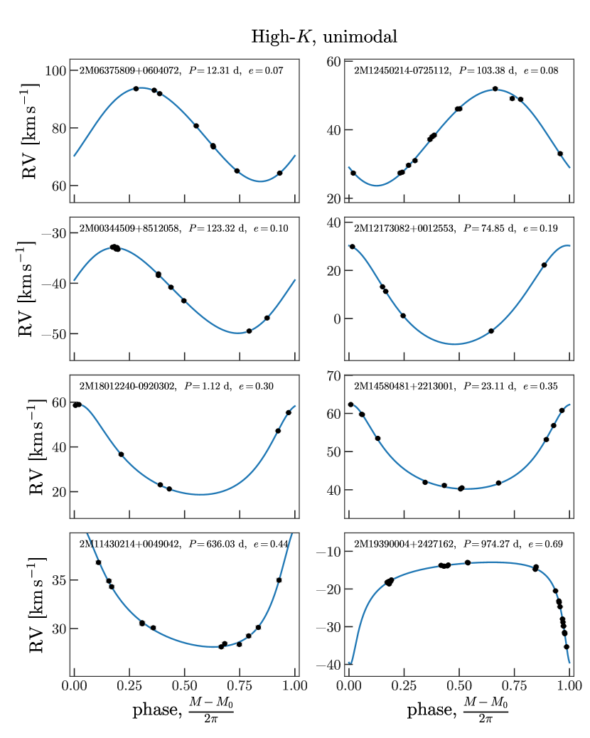
Figure 12: Randomly-selected examples of high-$K$ stars with effectively unimodal posterior samplings and converged MCMC samplings. Each panel shows the data (black markers), phase-folded at the period of the posterior sample with maximum posterior probability. Visit velocity uncertainties are shown as black error bars (these are typically smaller than or equal to the size of the markers), and the inferred jitter as grey, capped error bars. Line (blue) shows the orbit compute from the posterior sample with maximum posterior probability.

References

- Abolfathi et al. (2017) Abolfathi, B., Aguado, D. S., Aguilar, G., et al. 2017, ArXiv e-prints. https://arxiv.org/abs/1707.09322
- Astropy Collaboration et al. (2013) Astropy Collaboration, Robitaille, T. P., Tollerud, E. J., et al. 2013, A&A, 558, A33, doi: 10.1051/0004-6361/201322068
- Badenes et al. (2017) Badenes, C., Mazzola, C., Thompson, T. A., et al. 2017, ArXiv e-prints. https://arxiv.org/abs/1711.00660
- Bianchi et al. (2011) Bianchi, L., Herald, J., Efremova, B., et al. 2011, Ap&SS, 335, 161, doi: 10.1007/s10509-010-0581-x
- Blanton et al. (2017) Blanton, M. R., Bershady, M. A., Abolfathi, B., et al. 2017, AJ, 154, 28, doi: 10.3847/1538-3881/aa7567
- De Lee et al. (2013) De Lee, N., Ge, J., Crepp, J. R., et al. 2013, AJ, 145, 155, doi: 10.1088/0004-6256/145/6/155
- Duchêne & Kraus (2013) Duchêne, G., & Kraus, A. 2013, ARA&A, 51, 269, doi: 10.1146/annurev-astro-081710-102602
- Duquennoy et al. (1991) Duquennoy, A., Mayor, M., & Halbwachs, J.-L. 1991, A&AS, 88, 281
- Eggleton (1983) Eggleton, P. P. 1983, ApJ, 268, 368, doi: 10.1086/160960
- El-Badry et al. (2018) El-Badry, K., Ting, Y.-S., Rix, H.-W., et al. 2018, MNRAS, doi: 10.1093/mnras/sty240
- Foreman-Mackey et al. (2013) Foreman-Mackey, D., Hogg, D. W., Lang, D., & Goodman, J. 2013, PASP, 125, 306, doi: 10.1086/670067
- Foreman-Mackey et al. (2014) Foreman-Mackey, D., Hogg, D. W., & Morton, T. D. 2014, ApJ, 795, 64, doi: 10.1088/0004-637X/795/1/64
- Garcia & Stello (2018) Garcia, R. A., & Stello, D. 2018, ArXiv e-prints. https://arxiv.org/abs/1801.08377
- García Pérez et al. (2016a) García Pérez, A. E., Allende Prieto, C., Holtzman, J. A., et al. 2016a, AJ, 151, 144, doi: 10.3847/0004-6256/151/6/144
- García Pérez et al. (2016b) —. 2016b, AJ, 151, 144, doi: 10.3847/0004-6256/151/6/144
- Gelman & Rubin (1992) Gelman, A., & Rubin, D. B. 1992, Statistical Science, 7, 457, doi: 10.1214/ss/1177011136
- Goodman & Weare (2010) Goodman, J., & Weare, J. 2010, Communications in Applied Mathematics and Computational Science, Vol. 5, No. 1, p. 65-80, 2010, 5, 65, doi: 10.2140/camcos.2010.5.65
- Gunn et al. (2006) Gunn, J. E., Siegmund, W. A., Mannery, E. J., et al. 2006, AJ, 131, 2332, doi: 10.1086/500975
- Hekker et al. (2008) Hekker, S., Snellen, I. A. G., Aerts, C., et al. 2008, A&A, 480, 215, doi: 10.1051/0004-6361:20078321
- Hogg & Foreman-Mackey (2017) Hogg, D. W., & Foreman-Mackey, D. 2017, ArXiv e-prints. https://arxiv.org/abs/1710.06068
- Hogg et al. (2010) Hogg, D. W., Myers, A. D., & Bovy, J. 2010, ApJ, 725, 2166, doi: 10.1088/0004-637X/725/2/2166
- Huber (2017) Huber, D. 2017, Radial Velocity Oscillation Amplitudes of Kepler Stars, figshare, doi: 10.6084/m9.figshare.4887380.v1. https://figshare.com/articles/Radial_Velocity_Oscillation_Amplitudes_of_Kepler_Stars/4887380/1
- Huber et al. (2011) Huber, D., Bedding, T. R., Stello, D., et al. 2011, ApJ, 743, 143, doi: 10.1088/0004-637X/743/2/143
- Hunter (2007) Hunter, J. D. 2007, Computing In Science & Engineering, 9, 90
- Kipping (2013) Kipping, D. M. 2013, MNRAS, 434, L51, doi: 10.1093/mnrasl/slt075
- Kraus et al. (2008) Kraus, A. L., Ireland, M. J., Martinache, F., & Lloyd, J. P. 2008, ApJ, 679, 762, doi: 10.1086/587435
- Lloyd (1982) Lloyd, S. P. 1982, IEEE Transactions on Information Theory, 28, 129
- Majewski et al. (2017) Majewski, S. R., Schiavon, R. P., Frinchaboy, P. M., et al. 2017, AJ, 154, 94, doi: 10.3847/1538-3881/aa784d
- Martig et al. (2016) Martig, M., Fouesneau, M., Rix, H.-W., et al. 2016, MNRAS, 456, 3655, doi: 10.1093/mnras/stv2830
- Moe & Di Stefano (2017) Moe, M., & Di Stefano, R. 2017, ApJS, 230, 15, doi: 10.3847/1538-4365/aa6fb6
- Murray & Correia (2010) Murray, C. D., & Correia, A. C. M. 2010, Keplerian Orbits and Dynamics of Exoplanets, ed. S. Seager, 15–23
- Ness et al. (2015) Ness, M., Hogg, D. W., Rix, H.-W., Ho, A. Y. Q., & Zasowski, G. 2015, ApJ, 808, 16, doi: 10.1088/0004-637X/808/1/16
- Ness et al. (2016) Ness, M., Hogg, D. W., Rix, H.-W., et al. 2016, ApJ, 823, 114, doi: 10.3847/0004-637X/823/2/114
- Nidever et al. (2015) Nidever, D. L., Holtzman, J. A., Allende Prieto, C., et al. 2015, AJ, 150, 173, doi: 10.1088/0004-6256/150/6/173
- Pedregosa et al. (2011) Pedregosa, F., Varoquaux, G., Gramfort, A., et al. 2011, Journal of Machine Learning Research, 12, 2825
- Pérez & Granger (2007) Pérez, F., & Granger, B. E. 2007, Computing in Science and Engineering, 9, 21, doi: 10.1109/MCSE.2007.53
- Price-Whelan & Hogg (2017) Price-Whelan, A., & Hogg, D. W. 2017, adrn/thejoker: Release v0.1, doi: 10.5281/zenodo.264481. https://doi.org/10.5281/zenodo.264481
- Price-Whelan & Foreman-Mackey (2017) Price-Whelan, A. M., & Foreman-Mackey, D. 2017, The Journal of Open Source Software, 2, 357, doi: 10.21105/joss.00357
- Price-Whelan et al. (2017) Price-Whelan, A. M., Hogg, D. W., Foreman-Mackey, D., & Rix, H.-W. 2017, ApJ, 837, 20, doi: 10.3847/1538-4357/aa5e50
- Raghavan et al. (2010) Raghavan, D., McAlister, H. A., Henry, T. J., et al. 2010, ApJS, 190, 1, doi: 10.1088/0067-0049/190/1/1
- Serenelli et al. (2017) Serenelli, A., Johnson, J., Huber, D., et al. 2017, ApJS, 233, 23, doi: 10.3847/1538-4365/aa97df
- Ting et al. (2018) Ting, Y.-S., Hawkins, K., & Rix, H.-W. 2018, ArXiv e-prints. https://arxiv.org/abs/1803.06650
- Tokovinin (2014) Tokovinin, A. 2014, AJ, 147, 86, doi: 10.1088/0004-6256/147/4/86
- Tokovinin (2018) —. 2018, ApJS, 235, 6, doi: 10.3847/1538-4365/aaa1a5
- Troup et al. (2016) Troup, N. W., Nidever, D. L., De Lee, N., et al. 2016, AJ, 151, 85, doi: 10.3847/0004-6256/151/3/85
- Van der Walt et al. (2011) Van der Walt, S., Colbert, S. C., & Varoquaux, G. 2011, Computing in Science & Engineering, 13, 22, doi: http://dx.doi.org/10.1109/MCSE.2011.37