Multiple Superadiabatic Transitions and Landau-Zener Formulas

Abstract

We consider nonadiabatic systems in which the classical Born-Oppenheimer approximation breaks down. We present a general theory that accurately captures the full transmitted wavepacket after multiple transitions through either a single or distinct avoided crossings, including phase information and associated interference effects. Under suitable approximations, we recover both the celebrated Landau-Zener formula and standard surface-hopping algorithms. Our algorithm shows excellent agreement with the full quantum dynamics for a range of avoided crossing systems, and can also be applied to single full crossings with similar accuracy.

I Introduction

The Born-Oppenheimer approximation (BOA) Born and Oppenheimer (1927) is one of the most widely used methods used to study the quantum dynamics of molecules. Intuitively, it is motivated by the fact that the electrons are much lighter, and therefore much faster, than the nuclei, and hence rapidly adjust their positions with respect to those of the nuclei. This scale separation allows, in many cases, for the electronic and nuclear dynamics to be decoupled. In particular, if the electrons start in a certain bound state, for a fixed set of nuclei positions, then they should remain in this bound state even though the nuclei are slowly moving. Hence the nuclear dynamics can be determined by considering their motion on only one (electronic) potential energy surface.

However, there are interesting situations in which the BOA breaks down Domcke, Yarkony, and Horst (2004); Domcke, Yarkony, and Köppel (2011); Nakamura (2012); Tully (2012). For example, in many photochemical processes the nuclear motion cannot be restricted to a single potential energy surface because, for some nuclear configurations, two such surfaces become close, or even cross. In the former case, known as an avoided crossing, the BOA is still valid to leading order (in the small parameter $\epsilon$, which is the square root of the ratio of the electronic and nuclear masses), but the remaining corrections are of fundamental interest and, in fact, determine the associated chemistry. In the latter case, which generally takes the form of conical intersections, the BOA breaks down completely.

Here we are primarily interested in cases where the transmitted wavepacket is (exponentially) small  Hagedorn and Joye (2001, 2005); Martinez and Sordoni (2002), for example when there is an avoided crossing, or when the wavepacket does not pass directly over the conical intersection. Such regimes are, in some sense, generic, as avoided crossings are generic in 1D Von Neumann and Wigner (1929), and in higher dimensions the probability of an arbitrary wavepacket exactly hitting a conical intersection is vanishingly small Tully (2012). In particular, we consider cases where the wavepacket passes through multiple avoided crossings, or repeatedly through the same crossing. In such cases the transmitted wavepackets can interfere, and thus it is necessary to understand their phases. This suggests that a full quantum mechanical treatment of the problem is required. However, in even moderate dimensions, such treatments are numerically intractable, especially for multiple, coupled electronic potential surfaces.

In order to overcome this, a range of coupled quantum-classical and semiclassical methods have been developed. These include the multiple-spawning wavepacket method Ben-Nun and Martínez (1998); Ben-Nun, Quenneville, and Martínez (2000); Virshup, Chen, and Martínez (2012), the frozen Gaussian wavepacket method Heller (1991), Ehrenfest dynamics McLachlan (1964); Meyer and Miller (1979); Sawada, Nitzan, and Metiu (1985), and the semiclassical initial value representation Miller (1970); Kreek and Marcus (1974); Miller (2001). The main advantage of such schemes is the significantly reduced computational cost. The main disadvantage, at least with respect to the problem at hand, is the lack of phase information from almost all such schemes. Along with those mentioned above, one of the most widely-used quantum-classical approaches is surface hopping  Tully and Preston (1971); Miller and George (1972); Stine and Muckerman (1976); Kuntz, Kendrick, and Whitton (1979); Tully (1990); Hammes-Schiffer and Tully (1994); Müller and Stock (1997); Fabiano, Groenhof, and Thiel (2008); Fermanian Kammerer and Lasser (2008); Lasser and Swart (2008); Belyaev, Lasser, and Trigila (2014); Belyaev et al. (2015), in which particles are evolved under classical dynamics on a single surface and can ‘hop’ to other surfaces with a specified probability. Perhaps the most common approach is to only allow hops at points in the trajectory where the gap between energy surfaces has a local minimum (i.e. at an avoided crossing), and the probability of the hop is given by a Landau-Zener (LZ) formula Zener (1932); Landau (1965). Such methods give good results for a single transition, especially when the transmitted wavepacket is reasonably large, but fail completely when multiple transitions are involved, due to the complete lack of phase information Fermanian Kammerer and Lasser (2017). We note here that there is at least one such scheme Chai et al. (2015) that does aim to retain the phase information, but this is limited to small gaps between the potential energy surfaces, which in turn leads to large transmitted wavepackets. The same restriction is true for other mathematical approaches that lead to explicit formulae for the transmitted wavepacket; see e.g. Ref. Hagedorn and Joye (2005). It has been shown that, if the gap scales with $\epsilon$, then the transitions are of order one and dominated by the Landau-Zener factor Hagedorn (1994); Hagedorn and Joye (1998).

An alternative approach, inspired by the work of Berry on superadiabatic representations Berry (1990); Berry and Lim (1993), considers the full quantum mechanical wavepacket. These results, which are restricted to the semiclassical regime where the nuclei move classically, were later made rigorous Hagedorn and Joye (2004); Betz and Teufel (2005, 2005). It was later shown that, through the use of such superadiabatic representations (which are generalisations of the well-known adiabatic representation), it is possible to derive a formula for the transmitted wavepacket, including phase, at an avoided crossing  Betz, Goddard, and Teufel (2009); Betz and Goddard (2009, 2011); Betz, Goddard, and Manthe (2016). The associated algorithm requires only the quantum evolution of wavepackets on single energy surfaces. Whilst this is still computationally demanding if one wants to solve the full Schrödinger equation, there are approximate methods, such as Hagedorn wavepackets Hagedorn (1981, 1994); Lubich (2008) or standard quantum chemistry techniques such as MCTDH Huarte-Larrañaga and Manthe (2009), which make small relative errors and are computationally much more tractable. The associated algorithm has so far been applied to single transitions through avoided crossings Betz, Goddard, and Teufel (2009); Betz and Goddard (2009, 2011), and to multiple transitions of a single crossing in the case of the photodissociation of NaI Betz, Goddard, and Manthe (2016). The main goals here are to extend the methodology to multiple transitions through different avoided crossings and to systematically study the effects of making various approximations that lead to a LZ-like transition probability. We will also demonstrate that, although not designed to tackle such problems, the methodology can be successfully applied to single transitions of full crossings.

We present an algorithm that has a number of advantages. We have already mentioned: (i) Preservation of phase information, which allows the accurate study of interference effects; (ii) Only evolution on a single surface is required, which significantly reduces the computational cost when compared to a fully-coupled system, whilst also allowing the use of state-of-the art numerical schemes. The main other benefits are: (iii) Only the adiabatic surfaces (which are the most commonly obtained surfaces from quantum chemistry calculations) are required, in particular there is no need for a diabatization scheme, or the determination of the adiabatic coupling elements; (iv) Such surfaces are only required locally, and thus can be computed on-the-fly; (v) The transmitted wavepacket is created instantaneously, and hence there is no reliance on complicated numerical cancellations of highly-oscillatory wavepackets, which are generally present in the adiabatic representation; (vi) The methodology is easily extended to multiple adiabatic surfaces; (vii) The derived formula is accurate for a wide range of potential energy gaps and small parameters $\epsilon$, and for any semiclassical wavepacket, i.e. one of typical width or order $\sqrt{\epsilon}$.

There are, of course, also some disadvantages when compared to the more widely-used schemes: (i) In order to capture the phase information, the one-level dynamics must retain at least some of their quantum nature, and this is inherently more computationally demanding than the analogous classical dynamics; (ii) In the full formalism, it is necessary to be able to extend the potential surface into the complex plane, at least in the region of an avoided crossing. This is essential to be able to accurately compute the transition probabilities. However, in some regimes, for example when the LZ formula is accurate, we can bypass this requirement; (iii) The scheme is, in principle, restricted to wavepackets that are semiclassical near the avoided crossing. However, due to the linearity of the Schrödinger equation, and as demonstrated in Betz, Goddard, and Manthe (2016), it is possible to ‘slice’ the wavepacket at the crossing. However, this may be more problematic in higher dimensions; (iv) As it stands, the method is restricted to 1D. However, we have successfully extended it to higher dimensions through a slicing procedure [[REF 2D PAPER]].

To outline our approach, we will first review the standard model for nonadiabatic transitions (Section II) and avoided crossings (Section III). We will then, in Section IV, give a brief overview of existing surface hopping models and LZ formulas. We then outline the superadiabatic approach and give the resulting formula in Section V, before describing the associated algorithm in Section VI. In Section VII we systematically investigating its accuracy, and the effects of replacing the true transition probability by two LZ-like approximations. Finally, in Section VIII, we summarize our results and discuss some open problems.

II The Model

The Schrödinger equation governing the quantum dynamics of a molecular system can be written as

$${\rm i}\hbar\partial_{t}\psi({\boldsymbol{x}}_{\rm n},{\boldsymbol{x}}_{\rm e},t)=H_{\rm mol}\psi({\boldsymbol{x}}_{\rm n},{\boldsymbol{x}}_{\rm e},t),$$

where ${\boldsymbol{x}}_{\rm n}$ and ${\boldsymbol{x}}_{\rm e}$ are the nuclear and electronic positions, respectively, and the Hamiltonian is given by

$$H_{\rm mol}=-\frac{\hbar^{2}}{2m_{\rm n}}\Delta_{{\boldsymbol{x}}_{\rm n}}-\frac{\hbar^{2}}{2m_{\rm e}}\Delta_{{\boldsymbol{x}}_{\rm e}}+V_{\rm n}({\boldsymbol{x}}_{\rm n})+V_{\rm e}({\boldsymbol{x}}_{\rm e})+V_{{\rm n},{\rm e}}({\boldsymbol{x}}_{\rm n},{\boldsymbol{x}}_{\rm e}).$$

Here the first two terms are the kinetic energies of the nuclei and electrons with masses $m_{\rm n}$ and $m_{\rm e}$, respectively. Note that the masses of the nuclei may all be chosen to be the same by a rescaling of the nuclear coordinates. The potentials $V_{\rm n}$ and $V_{\rm e}$ denote the nuclear and electronic Coulomb repulsions, respectively, whilst $V_{\rm n,\rm e}$ is the attraction between the nuclei and electrons.

We now change to atomic units ($\hbar=m_{\rm e}=e=1$) and define $\epsilon=1/\sqrt{m_{\rm n}}$ and the electronic Hamiltonian for fixed nuclear positions ${\boldsymbol{x}}_{\rm n}={\boldsymbol{x}}$,

$$H_{\rm e}({\boldsymbol{x}})=-\frac{1}{2}\Delta_{{\boldsymbol{x}}_{\rm e}}+V_{\rm n}({\boldsymbol{x}})+V_{\rm e}+V_{{\rm n},{\rm e}}({\boldsymbol{x}},\cdot).$$

Suppose that $U^{\pm}({\boldsymbol{x}})$ are two eigenvalues of the electronic Hamiltonian (i.e. two adiabatic potential energy surfaces) of multiplicity one and well-separated from the rest of the electronic spectrum. Then, from Born-Oppenheimer theory Hagedorn (1980); Spohn and Teufel (2001), the effective nuclear Schrödinger equation is

$${\rm i}\epsilon\partial_{t}\psi({\boldsymbol{x}},t)=\Big{(}-\frac{\epsilon^{2}}{2}\Delta_{{\boldsymbol{x}}}+V({\boldsymbol{x}})\Big{)}\psi({\boldsymbol{x}},t),$$ (1)

where $V$ is a $2\times 2$ matrix with eigenvalues $U^{\pm}$, i.e. a diabatic matrix. In general, $V$ is symmetric and has the form

$$V({\boldsymbol{x}})=\begin{pmatrix}V_{1}({\boldsymbol{x}})&V_{12}({\boldsymbol{x}})\\ V_{12}({\boldsymbol{x}})&V_{2}({\boldsymbol{x}})\end{pmatrix}.$$

For notational convenience, and to connect back to previous work Betz, Goddard, and Teufel (2009); Betz and Goddard (2009, 2011); Betz, Goddard, and Manthe (2016), we find it useful to define

$$Z=(V_{1}-V_{2})/2,\quad X=V_{12},\quad d=(V_{1}+V_{2})/2,\quad\rho=\sqrt{X^{2}+Z^{2}}$$

and so

$$V({\boldsymbol{x}})=d({\boldsymbol{x}})+\begin{pmatrix}Z({\boldsymbol{x}})&X({\boldsymbol{x}})\\ X({\boldsymbol{x}})&-Z({\boldsymbol{x}})\end{pmatrix}.$$

It is easy to see that the adiabatic surfaces are then given by $U^{\pm}({\boldsymbol{x}})=d({\boldsymbol{x}})\pm\rho({\boldsymbol{x}})$ and so $\rho$ is half the energy gap between the two surfaces.

III Avoided Crossings

In the adiabatic representation, an explicit unitary transformation $U_{0}$ is applied to the system such that the electronic Hamiltonian is diagonal at each choice of ${\boldsymbol{x}}$. Transitions between the adiabatic surfaces are then governed by the kinetic energy term, which introduces off-diagonal coupling elements, giving (for a one-dimensional (1D) system) a Hamiltonian of the form

$$H_{0}=-\frac{\epsilon^{2}}{2}\partial_{x}^{2}+\begin{pmatrix}U^{+}(x)&-\epsilon\kappa(x)(\epsilon\partial_{x})\\ \epsilon\kappa(x)(\epsilon\partial_{x})&U^{-}(x)\end{pmatrix}+\mathcal{O}(\epsilon^{2}).$$ (2)

Here $\kappa=(X^{\prime}Z-Z^{\prime}X)/\rho^{2}$ is an explicit ‘kinetic coupling’ function and we have grouped the terms such that it is more obvious that the off-diagonal elements of the above matrix are of order $\epsilon$. This can be seen from the fact that wavepackets typically oscillate with frequency $1/\epsilon$ (see Section III), so $\epsilon\partial_{x}\psi(x)$ is of order one. Hence we see that, naïvely, the transitions are of order $\epsilon$ globally in time. However, as discussed previously, the transitions are exponentially small in $1/\epsilon$ away from the avoided crossings.

Typically, when the adiabatic potentials are well-separated, the coupling elements are small and then two levels may be treated separately via the Born-Oppenheimer approximation. However, if the adiabatic surfaces become close, but do not cross, the coupling terms typically become large (but do not diverge). Such nuclear configurations are known as avoided crossings. As a result of the large coupling elements, a small, but not negligible, part of the nuclear wavepacket is transferred between the adiabatic surfaces.

Suppose, for clarity of exposition, that the wavepacket initially occupies the upper adiabatic level. The aim of this work is to determine the transmitted wavepacket (on the lower adiabatic level) well away from the crossing (in the scattering regime). Whilst one can, in principle, compute this by a standard numerical solution of the Schrödinger equatiion, there are a number of challenges that prevent this from being a realistic option for most systems of interest:

1. In order to compute the dynamics, one needs an accurate representation of the potential energy surfaces. Typically the adiabatic surfaces are calculated using quantum chemistry methods, such as Density Functional Theory, but it is computationally expensive to determine such surfaces, especially when the number of degrees of freedom (dimension of ${\boldsymbol{x}}$) is large. In such cases, it is desirable to design methods that can utilise on-the-fly surfaces, determined only locally. Additionally, practical methods for determining surfaces for excited states are still in their infancy, and one also needs to determine the off-diagonal coupling elements. Finally, we note that diabatic representations are not unique, and those obtained in two- and multiple-level cases may differ significantly Belyaev et al. (2010).

2. The wavepackets we wish to compute are highly oscillatory, typically oscillating with frequency of order $\epsilon^{-1}$ in space. This can be seen by comparing the kinetic and potential terms in (1). When using a standard numerical scheme, such as Strang splitting, correctly resolving such oscillations requires very fine grids in both position and momentum space. The curse of dimensionality (for $N$ points in $d$ dimensions, one requires $N^{d}$ points) results in such approaches being impractical for all but very small dimensional systems.

3. Away from avoided crossings, the transmitted wavepacket is typically exponentially small in both the gap size $\delta$ and $1/\epsilon$. This can be seen from the formula (5) in Section V.2 or the standard LZ transition probabilities (3) and (4), where $\rho_{x_{c}}=\delta$. In contrast, globally in time, the transitions in the adiabatic representation are of order $\epsilon$, which we have already seen from the Hamiltonian 2. The necessary cancellations in the transmitted wavepacket occur through Stückelberg oscillations. See Figure 1 for an example. There are two challenges here. The first is to correctly resolve these cancellations, which can require very small time steps. The second is the more general challenge of computing an exponentially small quantity; any absolute errors in the numerical scheme must also be exponentially small or they will overwhelm the desired results.

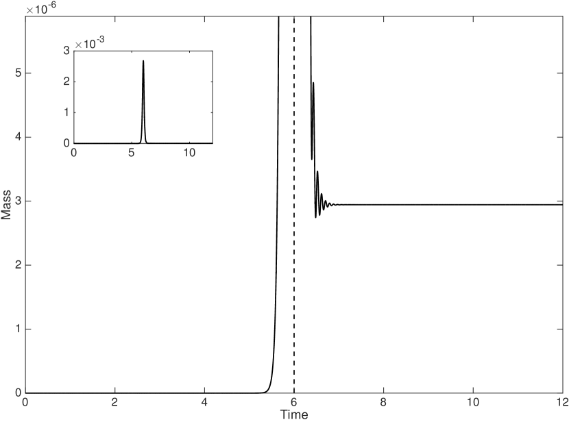
Figure 1: Inset: The mass of the transmitted wavepacket against time as the wavepacket on the original adiabatic surface moves through an avoided crossing. Main figure: Zoom for clarity of the final transmitted mass and Stückelberg oscillations. The time at which the centre of mass of the original wavepacket reaches the avoided crossing is marked with a dashed vertical line and coincides with the maximum transmitted mass.

IV Existing Approaches and Landau-Zener

In this section we discuss some existing approaches to calculate the transition probability or the transmitted wavepacket.

IV.1 Surface Hopping Algorithms

Here we present a brief overview of surface hopping methods, which are one of the most successful approaches for simulating nonadiabatic dynamics. Surface hopping is a mixed quantum-classical approach, where particles are transported classically on the adiabatic surfaces and hop between them under certain conditions, which simulates the quantum effects. A general surface hopping algorithm consists of four steps:

1. Sampling of the initial condition.

2. Classical evolution via $\dot{x}=p$, $\dot{p}=-\nabla U^{\pm}(x)$.

3. Surface hopping.

4. Computation of observables.

There are many such schemes, both deterministic and probabilistic and we refer to  Tully and Preston (1971); Miller and George (1972); Stine and Muckerman (1976); Kuntz, Kendrick, and Whitton (1979); Tully (1990); Hammes-Schiffer and Tully (1994); Müller and Stock (1997); Fabiano, Groenhof, and Thiel (2008); Fermanian Kammerer and Lasser (2008); Lasser and Swart (2008); Belyaev, Lasser, and Trigila (2014); Belyaev et al. (2015) for further details.

Of particular interest here is the surface hopping step. Typically this is performed when the gap between the two adiabatic surfaces is minimal along a classical trajectory. Whenever such a trajectory reaches a local minimum, a transition to the other surface is performed with a certain probability, usually derived from a simplified quantum mechanical model. The standard approach is to use a LZ formula, which we describe in the next section. The choice of this hopping probability is the main distinguishing feature of different surface hopping models.

The principal advantage of surface hopping algorithms is their simplicity. Due to their use of classical dynamics, which only require local properties of the potential energy surfaces, the methods can be applied in relatively high dimensions, using on-the-fly surfaces. As mentioned previously, such high dimensional systems are beyond the reach of full quantum mechanical methods.

The principal disadvantage is that they lose all phase information, and so cannot treat systems in which interference effects are important, or determine observables in which the relative phase of the wavepackets on the adiabatic surfaces is required Belyaev, Lasser, and Trigila (2014). Additionally, they are accurate only when the specified hopping probability is accurate; we will investigate this in Section VII.

IV.2 The Landau-Zener Formula

As mentioned previously, in order to compute the transition probability, it is common to use a LZ formula. Whilst the LZ model provides a simple formula for the transition probability, it is generally obtained from a one-dimensional, two-level model in the diabatic representation. However, practical applications occur in multiple dimensions and the potential energy surfaces are usually calculated in the adiabatic representation. There are a number of formulations of the LZ probability, including the extension to multiple dimensions in the diabatic formalism Fermanian Kammerer and Lasser (2008), and versions which only require knowledge of the adiabatic potentials  Zhu, Teranishi, and Nakamura (2001); Belyaev and Lebedev (2011). Here we restrict ourselves to two such formalisms, the first is a diabatic representation. which requires knowledge of the diabatic matrix elements, whilst the second is an adiabatic representation, which only requires the gap between the adiabatic potentials. From now on, we consider only 1D systems; see Section VIII for some discussion of progress in higher dimensions.

Consider a classical particle with trajectory $\big{(}x(t),p(t)\big{)}$ in phase space. Denote the position where $\rho$ attains a minimum by $x_{c}$, and the momentum of the particle at the corresponding time $t_{c}$ by $p_{c}$. Then the diabatic LZ transition probability is given by

$$P_{\rm d}=\exp\Big{(}-\frac{\pi}{\epsilon}\frac{\rho(x_{c})^{2}}{|p_{c}|\sqrt{X^{\prime}(x_{c})^{2}+Z^{\prime}(x_{c})^{2}}}\Big{)}.$$ (3)

The corresponding adiabatic transition probability is given by

$$P_{\rm a}=\exp\Big{(}-\frac{\pi}{\epsilon}\sqrt{\frac{\rho(x_{c})^{3}}{\frac{{\rm d}^{2}}{{\rm d}t^{2}}\rho(x(t))|_{t=t_{c}}}}\Big{)}.$$

If one has knowledge of the diabatic matrix elements, and hence $X$ and $Z$, this can be rewritten as

$$P_{\rm a}=\exp\Big{(}-\frac{\pi}{\epsilon}\frac{\rho(x_{c})^{2}}{|p_{c}|\sqrt{X^{\prime}(x_{c})^{2}+Z^{\prime}(x_{c})^{2}+X(x_{c})X^{\prime\prime}(x_{c})+Z(x_{c})Z^{\prime\prime}(x_{c})}}\Big{)}.$$ (4)

Note that in the corresponding multidimensional formula Belyaev, Lasser, and Trigila (2014) there is an additional term, which in 1D would be $[X(x_{c})X^{\prime}(x_{c})+Z(x_{c})Z^{\prime}(x_{c})](U^{\pm})^{\prime}(x_{c})$. However, since an avoided crossing is defined as a minimum of $\rho$, and $\rho^{\prime}=(XX^{\prime}+ZZ^{\prime})/\rho$, this term is zero in 1D.

V Superadiabatic Representations and the Formula

In this section we will briefly review the ideas behind the use of superadiabatic representations to compute the transmitted wavepacket and refer the reader to the cited works for more details. We will then present a generalisation of a previously-derived formula, which is applicable to 1D avoided crossings not centred at the origin.

V.1 Superadiabatic Representations

Superadiabatic representations were first introduced by Berry Berry (1990); Berry and Lim (1993), under the additional approximation that the nuclei move classically. More recently this has been extended to the full BOA  Betz, Goddard, and Teufel (2009); Betz and Goddard (2009, 2011); Betz, Goddard, and Manthe (2016). As suggested by the name, superadiabatic representations are refinements of the adiabatic representation, which we described in Section refS:avoidedCrossings. In the adiabatic representation, transitions can be very complicated, as demonstrated by the population on the lower level during a typical transition, see Figure 1. This reliance on large cancellations to leave an exponentially small wavepacket suggests that the adiabatic representation may not be the ideal frame of reference in which to study transitions at avoided crossings.

Superadiabatic representations improve on the adiabatic one by simplifying the dynamics near an avoided crossing, at the expense of introducing computational complexities. The superadiabatic representations can be enumerated, and, initially, moving to successively higher superadiabatic representations reduces the spurious oscillations in the dynamics until the transmitted population builds up monotonically as the wavepacket travels through the avoided crossing. This is known as the optimal superadiabatic representation. However, moving to even higher representations results in the spurious oscillations returning. Previous results give a reliable method to determine the optimal superadiabatic representation Betz, Goddard, and Teufel (2009); Betz and Goddard (2011). However, computing the unitary operators for this representation is highly challenging, and performing the numerical computations in such a representation is similarly difficult.

The main benefit of superadiabatic representations for our purposes is that they allow the derivation of an explicit formula for the transmitted wavepacket in the optimal superadiabatic representation, without requiring the associated unitary matrix. By general theory Teufel (2003), all of the superadiabatic representations agree with the adiabatic one away from any avoided crossing. This leads to a simple algorithm to compute the transition through an avoided crossing in the adiabatic representation, as described in Section VI.

V.2 The Formula

Following Ref. Berry and Lim (1993), it is useful to introduce a nonlinear rescaling in which the adiabatic coupling elements obtain a universal form, known as the natural scale,

$$\tau(x)=2\int_{x_{c}}^{x}\rho(s){\rm d}s,$$

where $x_{c}$ is the position of the avoided crossing. We now extend $\rho$ and $\tau$ into the complex plane and, by the theory of Stokes lines Joye, Mileti, and Pfister (1991), the analytic continuation of $\rho$ has a pair of complex conjugate zeros, close to $x_{c}$, at $x_{cz}$ and $x_{cz}^{*}$. We define

$$\tau_{x_{c}}=\tau(x_{cz})=\tau_{r}+{\rm i}\tau_{c}.$$

Let $\phi^{\pm}(x,t_{c})$ be the incoming wavepacket on the corresponding adiabatic surface $U^{\pm}$ at time $t_{c}$ when the centre of mass coincides with an avoided crossing at $x_{c}$. Then, for $t>t_{c}$, the transmitted wavepacket on the other adiabatic surface $U^{\mp}$ can be approximated by

$$\psi(x,t)=\,{\rm e}^{-({\rm i}/\epsilon)(t-t_{c})H^{\mp}}\,\psi^{\mp}(x)$$

where $H^{\mp}$ are the BOA Hamiltonians for the two levels and $\psi^{\mp}(x)$ is a wavepacket instantaneously created at time $t_{c}$, which is more easily expressed in Fourier space via

$$\hat{\psi}^{\mp}(p) =\Theta(p^{2}\mp 4\delta)\frac{p+\eta^{\mp}}{2|\eta^{\mp}|}\exp\Big{(}-\frac{\tau_{c}}{2\delta\epsilon}|p-\eta^{\mp}|\Big{)}\exp\Big{(}-{\rm i}\frac{\tau_{r}}{2\delta\epsilon}(p-\eta^{\mp})\Big{)}$$

$$\qquad\times\exp\Big{(}-{\rm i}\frac{x_{c}}{\epsilon}(p-\eta^{\mp})\Big{)}\hat{\phi}^{\pm}(\eta^{\mp}).$$ (5)

Here

$$\delta=\rho(x_{c}),\quad\eta^{\mp}={\operatorname{sign}}(p)\sqrt{p^{2}\mp 4\delta},$$

$\Theta$ is the Heaviside function and the Fourier transform needs to be performed under the correct scaling:

$$\hat{\psi}(p)=\frac{1}{2\pi\epsilon}\int\,{\rm e}^{-({\rm i}/\epsilon)px}\,\psi(x){\rm d}x.$$

We note that the principle difference from previous presentations of the formula is the final exponential factor involving $x_{c}$, the position of the avoided crossing. In previous work, this position has been taken to be zero, in which case the factor is simply 1. The new term arises from the approximation $x(\tau)=\tau/(2\delta)+x_{c}+\mathcal{O}(\tau^{3})$ (which is a simple generalisation of the calculation for $x_{c}=0$ (Betz and Goddard, 2011, p. 2258)).

V.3 Analysis of the Formula

We now present a brief analysis of the formula in 5, which allows us to connect to surface hopping approaches, as well as to LZ formulas.

Firstly we note that the formula involves the same momentum adjustment that is phenomenologically introduced in surface hopping algorithms. We note that $\eta\mp$ is precisely the classical incoming momentum required to give outgoing momentum $p$ when moving down/up, respectively, a potential energy gap of $2\delta$ and requiring (classical) energy conservation. Relatedly, when passing from the upper to the lower level, the Heaviside function ensures that the transmitted wavepacket has (absolute) momentum at least $2\delta$, whereas when passing from the lower to upper level it is trivially 1, indicating no restriction on the transmitted momentum. The analogous restriction that a classical particle can only be transmitted to the upper level if it has sufficient kinetic energy is accounted for by the $\hat{\psi}^{\pm}(\eta^{\mp})$ term.

We now discuss how, in appropriate limits, the formula essentially reduces to a LZ transition for each point in momentum space. We make a number of independent approximations:

1. $x_{c}=0$.
   For a single avoided crossing we may do this without loss of generality by shifting the space variable.

2. $\tau_{r}=0$.
   This is the case, for example, when the potential is symmetric around the avoided crossing.

3. $\delta$ is small.
   This produces two simplifications to the formula using that $\eta^{\mp}\approx p\mp 2\delta/p$:

   • The prefactor simplifies to $\frac{\eta^{\mp}+p}{2|\eta^{\mp}|}\approx p/|p|={\operatorname{sign}}(p)$;

   • The factor in the exponential simplifies to $|p-\eta^{\mp}|\approx 2\delta/|p|$.

   Note that the small parameter in these expansions is actually $\delta/p_{0}$, and so we expect these approximations to be more accurate for either small $\delta$ or large incoming momentum.

4. Second order expansion of $\rho$.
   It is well known Berry and Lim (1993) that a naïve second order expansion of $\rho$ is incorrect as the analytic continuation of $\rho$ must vanish like a square root at its complex zeros. We therefore approximate $\rho$ via

   $$\rho(x)\approx\sqrt{\delta^{2}+g(x-x_{c})}$$

   with $g$ a smooth function such that $g(0)=g^{\prime}(0)=0$. Performing a second order expansion of $g$ then gives

   $$\rho(x)\approx\sqrt{\delta^{2}+\tfrac{1}{2}g^{\prime\prime}(0)(x-x_{c})^{2}}.$$

   In this case both $x_{cz}$ and $\tau_{c}$ can be computed analytically to give

   $$\tau_{c}\approx{\rm i}\frac{\pi\delta^{2}}{2\alpha}$$

   where $\alpha^{2}=\tfrac{1}{2}g^{\prime\prime}(0)$. To connect purely to $\rho$, we note that $\frac{1}{2}g^{\prime\prime}(0)=\delta\rho^{\prime\prime}(x_{c})$ and hence

   $$\tau_{c}\approx{\rm i}\frac{\pi\delta^{3/2}}{2\sqrt{\rho^{\prime\prime}(x_{c})}}.$$

   Finally, in order to connect to the LZ formulas, an explicit computation using that $\rho^{\prime}(x_{c})=(X(x_{c})X^{\prime}(x_{c})+Z(x_{c})Z^{\prime}(x_{c}))/\rho(x_{c})=0$ and $\rho(x_{c})=\delta$ gives

   $$\rho^{\prime\prime}(x_{c})=\frac{X^{\prime}(x_{c})^{2}+Z^{\prime}(x_{c})^{2}+X(x_{c})X^{\prime\prime}(x_{c})+Z(x_{c})Z^{\prime\prime}(x_{c})}{\delta}$$

   and so

   $$\tau_{c}\approx{\rm i}\frac{\pi\delta^{2}}{2\sqrt{X^{\prime}(x_{c})^{2}+Z^{\prime}(x_{c})^{2}+X(x_{c})X^{\prime\prime}(x_{c})+Z(x_{c})Z^{\prime\prime}(x_{c})}}.$$

Suppose now that we make all four approximations. Then the formula in (5) becomes

$$\hat{\psi}^{\mp}(p)={\operatorname{sign}}(p)\Theta(p^{2}\mp 4\delta)\exp\Big{(}-\frac{\pi\delta^{2}}{2\epsilon|p|\sqrt{X^{\prime}(x_{c})^{2}+Z^{\prime}(x_{c})^{2}+X(x_{c})X^{\prime\prime}(x_{c})+Z(x_{c})Z^{\prime\prime}(x_{c})}}\Big{)}\hat{\psi}^{\pm}(\eta^{\mp}).$$ (6)

It is now clear that the exponential factor corresponds precisely to the adiabatic LZ transition probability in (4), with the additional factor of $1/2$ accounting for the fact that we are determining the size of the transmitted wavepacket rather than the transition probability, which is proportional to the square of the wavepacket. The Heaviside function is also included indirectly in surface hopping models, which explicitly exclude classically-forbidden transitions, see e.g. Belyaev, Lasser, and Trigila (2014).

Note that if we are interested solely in the transition probability then the first two approximations are irrelevant as they only affect the phase. However, when dealing with multiple transitions these terms are crucial in understanding interference effects. In Section VII we will investigate the effects of these approximations in some example systems.

After approximations (1)–(4) have been made, the resulting formula (6) can be thought of as a surface hopping algorithm that retains phase information. This can be seen by noting that the formula decouples in momentum space. Thus, if we replace the classical transport of individual particles, the ensemble of which represents the initial wavepacket, with quantum evolution of the initial wavepacket, and then replace particle hopping with hopping of momentum components of the wavepacket, then we have a clear analogue of the surface hopping methods. One promising avenue of further work is to investigate the use of formula 5 for the transmission probability (instead of the LZ one) in traditional surface hopping algorithms. Alternatively, we can recover the surface hopping methodology (but retaining phase information) by dividing the wavepacket into small pieces (the surface hopping particles), evolving them classically on the initial level (e.g. using Hagedorn’s wavepacket approach Hagedorn (1981, 1994); Lubich (2008)) until they reach an avoided crossing, and then applying the formula either with the full transition probability, or the LZ approximation, and reconstructing the wavepacket on the other level.

VI The Algorithm

The general algorithm described below is similar to that presented in previous work, but here it is extended to multiple transitions and to different levels of approximation, which ultimately lead to an analogue of the LZ formula, but applied to wavepackets, rather than simply as a transition probability. The transmitted wavepacket is computed via the following algorithm. For clarity, we present the algorithm for two BOA surfaces, but its extension to multiple surfaces is straightforward due to the linearity of the Schrödinger equation.

1. Initial Condition: The initial wavepacket should be specified on either the upper or lower adiabatic level, well away from any of the avoided crossings. Note that, in such regions, the adiabatic, superadiabatic, and diabatic levels are very close, so one may instead specify the wavepacket on a single diabatic level. If the initial wavepacket is given close to an avoided crossing, for example as the result of a laser excitation, then it must be evolved away (into the scattering regime) on the corresponding adiabatic level under the BO approximation to obtain an appropriate initial wavepacket.

2. One-Level Dynamics: The initial wavepacket is now evolved under the BOA until the final, specified time, or until another termination condition is satisfied (such as the wavepacket reaching a minimum distance from an avoided crossing). This can be done using any one-level scheme that provides sufficient accuracy, such as Strang splitting, Hagedorn wavepackets Hagedorn (1981, 1994); Lubich (2008), or MCTDH Huarte-Larrañaga and Manthe (2009). The wavepacket on the other BOA level is evolved simultaneously; the level is initially unoccupied.

3. Detection of Avoided Crossings: Here an avoided crossing is defined as a (local) minimum of the gap $\rho$. Whenever the centre of mass of the wavepacket reaches such a minimum, apply the formula as described in the next step. Such local minima may be determined a priori, for example when the potentials are given analytically, or on-the-fly by monitoring $\rho$.

4. Application of the Formula: Apply the formula (5) to the wavepacket at the avoided crossing and add the resulting wavepacket to the lower level. Note that the formula implicitly requires the potentials to be extended into the complex plane in order to compute $\tau$. However, as described in the following Section, this requirement may be bypassed by using an analogue of the Landau-Zener formula, at a cost to accuracy which is investigated for some examples in Section VII.

5. Computation of Observables: At any time step the wavepackets on the two levels may be used to compute observables, such as mean position, momentum and the level populations, including those which require phase information such as inter-level observables. Note, however (as discussed in Section V.1), that these will only agree with the corresponding quantities computed for the adiabatic populations well away from any avoided crossings. An extreme example of this is that, before the wavepacket on the initial level reaches the avoided crossing, the other level us completely unoccupied; see Figure 8.

In the following section we will investigate the accuracy of this algorithm. One restriction for its application to multiple crossings is that the transmitted wavepacket must be small, or, more precisely, the wavepacket remaining on the original surface must not change significantly when compared to its evolution under the BOA. This is due to the perturbative nature of the derivation, which assumes that the original wavepacket is unchanged during a transition.

VII Numerics

Note that the MATLAB code used to produce the results in this section is available from https://bitbucket.org/bdgoddard/qmd1dpublic/.

VII.1 Jahn-Teller

We consider first a simple example in order to demonstrate the effects of the approximations in Section V.3. We choose

$$V(x)=\begin{pmatrix}x&\delta\\ \delta&-x\end{pmatrix}$$

where we have $X=\delta$, $Z=x$, $\rho=\sqrt{x^{2}+\delta^{2}}$. There is a single avoided crossing at $x_{c}=0$, with gap $2\delta$. It is clear that $x_{cz}={\rm i}\delta$ and a straightforward calculation shows that $\tau_{x_{c}}={\rm i}\delta^{2}\pi/2$. Note, therefore, that assumptions (1), (2) and (4) of Section V.3 hold exactly. Furthermore, since $X(x_{c})X^{\prime\prime}(x_{c})+Z(x_{c})Z^{\prime\prime}(x_{c})=0$, the diabatic and adiabatic LZ transition probabilities given in (3) and (4) are identical in this case. This simple model allows us to investigate the effects of approximation (3), i.e. the difference between the full formula (5) and the LZ approximation for a range of values of $\delta$. From the arguments in Section V.3, we expect the two results to agree to high accuracy when $\delta/p_{0}$ is small, and hence the transition is large, but we expect the full formula result to be more accurate in the regime of interest (relatively large $\delta$ and small transitions).

We choose to specify the wavepacket at the avoided crossing, and determine the initial condition by evolving it backwards in time away from the crossing on a single adiabatic surface. This ensures that the wavepacket is semiclassical (i.e. of width order $\sqrt{\epsilon}$) when it reaches the avoided crossing. As noted above, due to the linearity of the Schrödinger equation, if this were not the case then we could apply a slicing procedure to obtain similarly accurate results. In particular, we choose

$$\hat{\psi}(p)=\frac{1}{(\pi\epsilon)^{1/4}}\exp\Big{(}-\frac{{\rm i}}{\epsilon}p_{0}x_{0}-\frac{1}{2\epsilon}(p-p_{0})^{2}-\frac{{\rm i}}{\epsilon}x_{0}(p-p_{0})\Big{)}$$ (7)

where, along with $\delta$, the free parameters are $\epsilon$ and $p_{0}$. For this example we fix $\epsilon=1/50$, which is similar to the value chosen in surface hopping works e.g. Fermanian Kammerer and Lasser (2008); Belyaev, Lasser, and Trigila (2014); Fermanian Kammerer and Lasser (2017) (and approximately correct for real-world systems e.g. Betz, Goddard, and Manthe (2016)) and $p_{0}=8$. We could, in principle, vary these parameters, and we will do so in later examples. We note that due to the nature of the potential, in order to start sufficiently far away from the avoided crossing (such that the adiabatic and superadiabatic representations agree) the initial potential energy must be reasonably large, leading to a correspondingly large minimum value of $p_{0}$ at the avoiding crossing. See Figure 3 for the adiabatic potentials.

Here we evolve backwards to a start time of $-40/p_{0}$ with timestep $1/(1000p_{0})$ and then forwards through the avoided crossing for time $80/p_{0}$ with the same timestep. We perform the numerics with a spatial grid with $2^{15}$ points and endpoints $\pm 60$. We observe that halving the time step and doubling the number of grid points does not significantly affect the results.

In Figure 2 we show the relative error in the transmitted wavepacket and the transmitted mass. This clearly demonstrates that, for small $\delta$ (and large transmitted mass), both our formula (5) and the LZ-like version (6) give very good results. However, as $\delta$ increases, the simplified version becomes increasingly inaccurate.

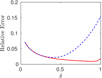
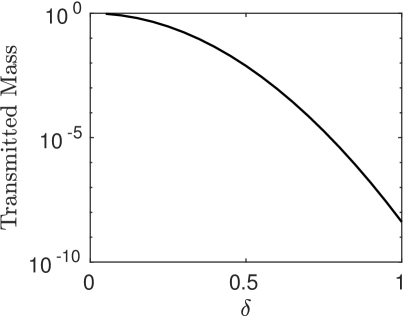
Figure 2: Left: The relative error between the ‘exact’ numerical solution and the application of the algorithm using formula (5) [red, solid] and (6) [blue, dashed]. Right: The ‘exact’ transmitted mass, which is in excellent agreement with that computed using (5) for all values of $\delta$.

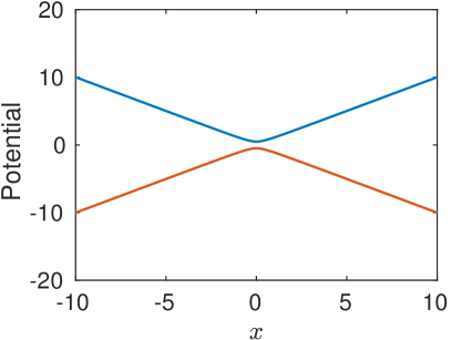
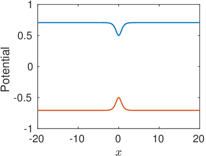
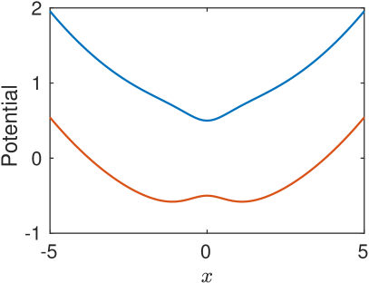
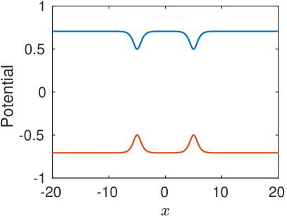
Figure 3: The adiabatic potentials for [clockwise from top left] the Jahn-Teller, Simple, Dual and Quadratic Potentials

.

VII.2 Simple Avoided Crossing

We now consider a simple example, which will both allow us to systematically investigate the accuracy of our method for different parameter regimes, and provide a benchmark for the accuracy of a single transition; this is, at least heuristically, a lower bound for the accuracy for multiple transitions. We choose

$$V(x)=\begin{pmatrix}\tfrac{1}{2}\tanh(x)&\delta\\ \delta&-\tfrac{1}{2}\tanh(x)\end{pmatrix}$$

where we have $X=\delta$, $Z=\tfrac{1}{2}\tanh(x)$, $\rho=\sqrt{\tfrac{1}{4}\tanh(x)^{2}+\delta^{2}}$. See Figure 3 for the adiabatic potentials with $\delta=1/2$.

As in the previous example, in order to control the (mean) momentum of the wavepacket when it reaches the crossing, we specify the wavepacket in momentum space at the avoided crossing and then evolve it backwards in time on a single adiabatic surface to obtain an initial wavepacket for the computations. In particular, we take a Gaussian wavepacket as given in (7) for a range of values of $\epsilon$ and $p_{0}$. We compute the results for a single transition of the avoided crossing, both using the full formula (5) and the LZ-like one (6). As can be seen from Figure 4, the relative error when using 5 is typically of the order of a few percent, with increasing accuracy as $\delta$ and/or $p_{0}$ increase. The deviation of the green curve, which corresponds to $\epsilon=1/10$ is a result of the asymptotic nature of the formula. The odd behaviour of the blue curve for $p_{0}=3$, $\epsilon=1/50$ and $\delta\approx 1$ seems to be a result of parts of the wavepacket becoming ‘trapped’ near the avoided crossing, which violates the assumption of a single transition.

Figures 5 and 6 demonstrate the effects of using the algorithm with the approximate formula (6). As can be seen from Figure 5, for moderate values of $\delta$, the results become very poor. However, as expected, Figure 6 shows that, for small $\delta$, the results are very similar to those using the full formula (5).

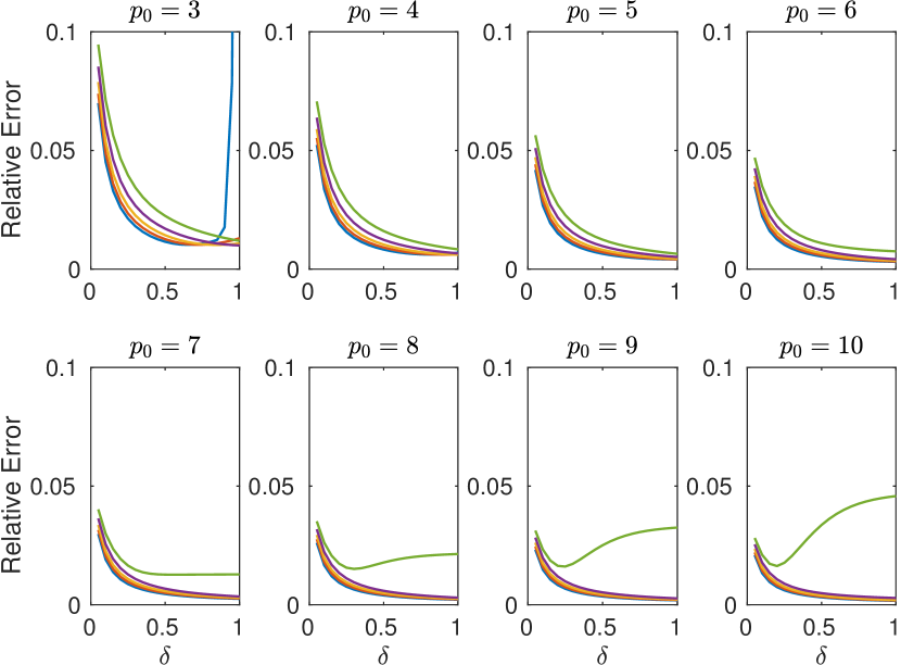
Figure 4: The relative error between the ‘exact’ numerical solution and the application of the algorithm using formula (5). Each subplot shows the result for a different value of $p_{0}$ for a range of $\delta$ values. Different colour curves $\{$green, purple, yellow, red, blue$\}$ correspond to $\epsilon=\{1/10,1/20,1/30,1/40,1/50\}$, respectively. Note that, apart from the largest value $\epsilon=1/10$, the errors are very similar.

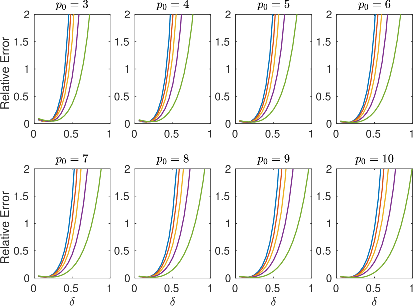
Figure 5: As Figure 4 but using formula (6). Note that the results for all but the smallest values of $\delta$ are significantly worse than those in Figure 4.

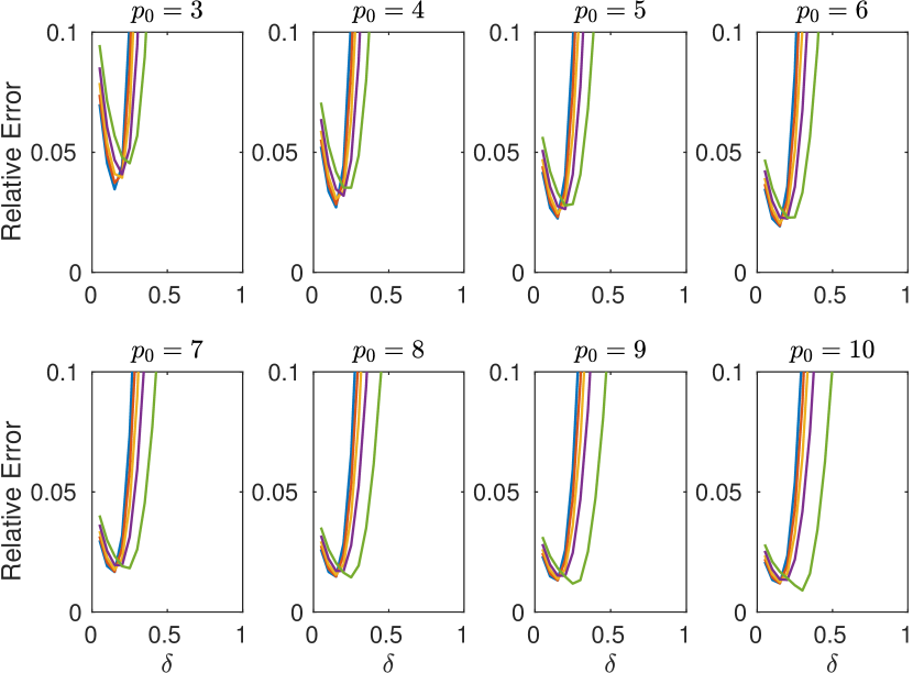
Figure 6: Zoom of Figure 5.

For completeness, we give the numerical details: The spatial grid uses $2^{14}$ points with limits $\mp 40$. We use a time step of $1/(100p_{0})$ and obtain the initial wavepacket by evolving the wavepacket backwards from the crossing for time $20/p_{0}$. The system is then evolved forwards for time $40/p_{0}$. Again, we note that halving the time step and doubling the number of grid points does not significantly affect the results.

As a further test of the accuracy of the algorithm we perform the same calculation as for the Gaussian wavepackets in the previous example, but with a wavepacket on the upper level at the crossing given by

$$\hat{\psi}(p)=\sum_{j=1}^{3}w_{i}\hat{\psi}(x_{0,i},p_{0,i},p),$$ (8)

where $\hat{\psi}$ is a Gaussian as given by (7). We choose $\epsilon=1/50$, $w=[0.7,1,0.9]$, $p_{0}=[4.6,5,5.3]$ and $x_{0}=[0.1,0,-0.05]$. However, we note that the results are robust under these choices for a wide range of values. We show the resulting transmitted wavepacket in Figure 7 which for convenience of displaying the phase, we have evolved backwards to the avoided crossing on the lower level. Note that the relative error in this case is 0.0057. In particular, Figure 7 demonstrates that higher-momentum wavepackets are more likely to make the transition.

We note here that the results for wavepackets starting on the lower level are very similar, and we will investigate such a situation in the following Section.

VII.2.1 Full Crossings

Here we consider if the algorithm is applicable to full crossings (with $\delta=0$). In such a case, the approximations made in Section V.3 lead to the conclusion that the transmitted wavepacket is approximately equal to the incoming wavepacket. Applying this in the case $p_{0}=5$, $\epsilon=1/50$ and $\delta=0$ gives a relative of 0.0856 for both the formula (5) and LZ approximation (6). This is comparable to the relative error for small, but non-zero $\delta$ (see Figure 4). This indicates that the methodology can also be used for full crossings. This is important in higher dimensions, where part of the wavepacket may travel across a full crossing (conical intersection), whilst other parts experience an effective avoided crossing, in which case we need only one algorithm to accurately treat the whole wavepacket.

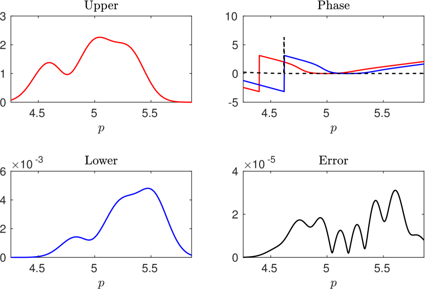
Figure 7: The wavepacket in momentum space. ‘Upper’ denotes the wavepacket on the upper level at the avoided crossing, as given by (8). ‘Lower’ denotes the transmitted wavepacket, computed using the algorithm, evolved backwards on the lower level to the avoided crossing. ‘Phase’ shows the phase of the upper (red), lower (blue) and error, for the lower, transmitted phase (black, dashed). ‘Relative Error’ displays the relative error between the transmitted wavepackets given by the ‘exact’ solution and the result of the algorithm.

VII.2.2 Diabatic vs. Adiabatic LZ

In the previous examples, we have $X(x_{c})X^{\prime\prime}(x_{c})+Z(x_{c})Z^{\prime\prime}(x_{c})=0$ and hence the diabatic and adiabatic LZ transition probabilities, (3) and (4), respectively, are identical. However, here we briefly consider an example in which this is not the case. We note that such a situation was also investigated in Ref. Belyaev, Lasser, and Trigila (2014) for two-dimensional crossings and the results when using the two formalisms were found to be very similar. We will now show that this is not always the case. We take a sightly perturbed version of the simple potential matrix above

$$V(x)=\begin{pmatrix}\tfrac{1}{2}\tanh(x)&\delta+\tfrac{1}{10}\tanh^{2}(x)\\ \delta+\tfrac{1}{10}\tanh^{2}(x)&-\tfrac{1}{2}\tanh(x)\end{pmatrix},$$

i.e $X=\delta+\tfrac{1}{10}\tanh^{2}(x)$ and $Z=\tfrac{1}{2}\tanh(x)$. We choose $\delta=0.2$, $\epsilon=1/50$ and $p_{0}=5$ where these parameters, are chosen such that we are in a regime where we expect both the formula (5) and the (adiabatic) LZ approximation to be reasonably accurate, whilst simultaneously the results are not dominated by $\delta$ being very small. We use the same numerical scheme as for the simple crossing above and, find that the relative errors when using the formula (5) and the adiabatic LZ approximation (4) (or (6)) are very similar at 0.0219 and 0.0217, respectively. In contrast, when using the diabatic approximation (3), the results are much worse, with a relative error of 0.1081. This, along with previous results, demonstrates a clear motivation to use the transition formula in surface hopping algorithms.

VII.3 Multiple Transitions of a Single Crossing

We now demonstrate the algorithm when the wavepacket makes multiple transitions of a single avoided crossing. Here we add a quadratic confining potential, which causes the wavepacket to oscillate backwards and forwards through the avoided crossing:

$$V(x)=\alpha x^{2}+\begin{pmatrix}\tfrac{1}{2}\tanh(x)&\delta\\ \delta&-\tfrac{1}{2}\tanh(x)\end{pmatrix},$$

where $X=\delta$, $Z=\tfrac{1}{2}\tanh(x)$, $\rho=\sqrt{\tfrac{1}{4}\tanh(x)^{2}+\delta^{2}}$ and $d(x)=\alpha x^{2}$. We choose $\alpha=0.05$, which gives a relatively weak confining potential. We use the same grid and time step as for the simple case in Section VII.2 but here evolve back to $t=-5$ and forwards to $t=30$, which gives 3 complete transitions of the avoided crossing. Here we start with a wavepacket of the form (7) on the lower level with $x_{0}=0$ and $p_{0}=5$. Again we choose $\epsilon=1/50$. See Figure 3 for the adiabatic potentials.

As can be seen in Figure 8, the ‘exact’ dynamics require extreme numerical cancellations at each transition in order to produce the true wavepacket. Although not shown in the Figure, the maximum transmitted mass is 0.0028, which is around 200 times larger than the final mass. Note that the results of both formulas are of a similar accuracy to the results for a single crossing, with relative errors 0.0123 and 3.637 for (5) and (6), respectively. In particular, the agreement between the ‘exact’ and formula (5) results is excellent whilst, in this case, (6) significantly underestimates the size of the transmitted wavepackets.

Whist, in principle, we would expect the results of using (6) to improve when $\delta$ decreases (i.e. when the transmitted wavepacket is larger) this adds a complication to the algorithm: When the transmitted wavepacket is large, the transition significantly affects the wavepacket on the original level, which is used explicitly in the formula for the transmitted wavepacket at the next avoided crossing. Due to the perturbative nature of the derivation of the formula (5) (see e.g. Betz, Goddard, and Teufel (2009); Betz and Goddard (2009)), the wavepacket on the original level is not treated explicitly, and so we do not have access to this unless it can be assumed that it is largely unaffected by the transition. A necessary requirement for this, due to mass conservation, is that the transmitted wavepacket is small.

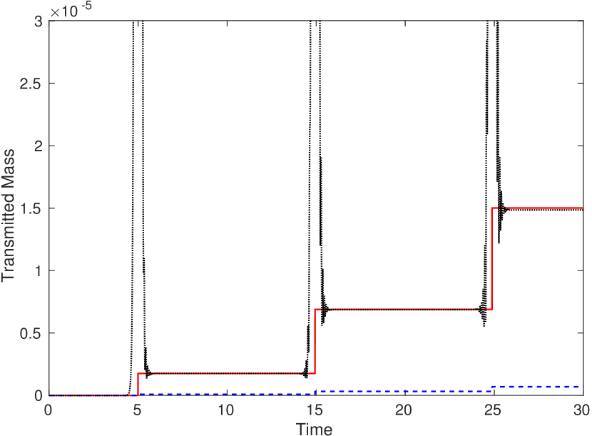
Figure 8: Mass of transmitted wavepacket on the upper adiabatic level over time for the ‘exact’ dynamics [black, dotted] and using the algorithm with formulas (5) [red, solid] and (6) [blue, dashed]. The centre of mass of the wavepacket on the lower level reaches the avoided crossing three times, at approximately $t=5,15,25$, as indicated by the jumps in the formula masses.

VII.4 Dual Avoided Crossings

As we have seen, for multiple transitions at a single avoided crossing, the algorithm described in Section VI works as expected, determining the correct phase of the wavepackets, and therefore also the correct interference effects. However, for transitions at separate avoided crossings there is an extra difficulty that arises from the definition of the diabatic and adiabatic potentials. As can be seen from Figure 9, in an example with two identical avoided crossings at $\pm x_{c}$, the diabatic eigenfunctions are even. Hence, treating the two crossings independently, the dynamics through the second crossing could be computed by flipping the surfaces in space (which gives the diabatic surfaces associated with the first crossing) and reversing the momentum of the wavepacket. From (5), we see that reversing the momentum introduces a sign change in the transmitted wavepacket, which must be taken into account when computing the total transmitted wavepacket. (This issue is related to the diabatic eigenfunctions only being defined up to their sign.) Note that this argument generalises to the case where there are multiple non-identical crossings; the case here was chosen for clarity.

Here we choose potentials

$$V(x)=\begin{pmatrix}\tfrac{1}{2}\big{(}\tanh(x-5)+\tanh(x+5)+1\big{)}&\delta\\ \delta&-\tfrac{1}{2}\big{(}\tanh(x-5)+\tanh(x+5)+1\big{)}\end{pmatrix}$$

where we have $X=\delta$ and $Z=\tfrac{1}{2}\big{(}\tanh(x-5)+\tanh(x+5)+1\big{)}$. We choose $\epsilon=1/50$, $\delta=1/2$ and an initial Gaussian condition using (7) with $x_{0}=0$ and $p_{0}=5$. We use the same numerical scheme as in Section VII.2], first evolving backwards for $t=5$ and then forwards for $t=10$. See Figure 3 for the adiabatic potentials.

As can be seen from Figure 10, the results using (5) are once again very good (with a relative error of 0.0295), whilst those using the approximate formula (6) are much poorer (relative error 2.193). Note that if we do not include the additional phase correction described above then the results using (5) are also very poor.

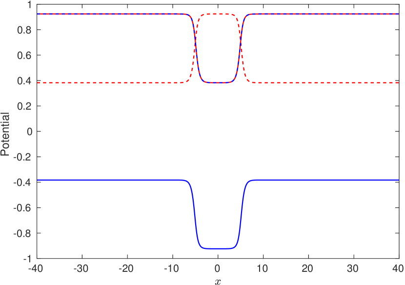
Figure 9: Components of the two diabatic eigenvectors $\Phi_{1}$ and $\Phi_{2}$ in red and blue, respectively. Solid and dashed lines show the two components, denoted by $\Phi_{j}^{\pm}$. Note that $\Phi_{1}^{+}=\Phi_{2}^{-}$ and $\Phi_{2}^{+}=-\Phi_{1}^{-}$. The avoided crossings are at $x\approx\pm 5$.

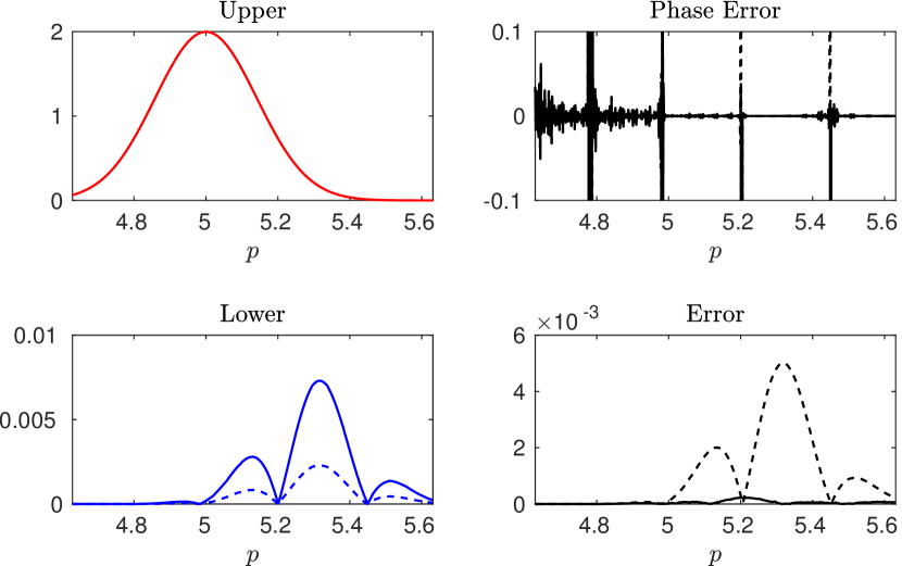
Figure 10: Top left: The final wavepacket on the upper level. Bottom left: The final transmitted wavepackets on the lower level using (5) [solid] and (6) [dashed]. Bottom right: The associated errors when compared to the ‘exact’ numerical solution. Top right: The phase error, which is very small in both cases apart from when the amplitude of the wavepacket is very small.

VIII Conclusions and Open Problems

We have presented a general scheme for the computation of wavepackets transmitted during multiple transitions through avoided crossings (at least when the transmitted wavepacket is small), which is also applicable to single transitions through full crossings. In fact, since, in the latter case, almost the entire wavepacket is transmitted, the scheme should also give accurate results for multiple transitions of full crossings, or combinations of a single full and multiple avoided crossings.

The principal advantage of our algorithm is that it produces the full quantum wavepacket, including its phase, in particular allowing the investigation interference effects during multiple transitions. This is in contrast to standard surface-hopping algorithms that lose all phase information, and cannot hope to treat systems with interference effects.

Open problems, which will be the subject of future works, are (i) Approximation of the wavepacket that remains on the original level when the transmitted wavepacket is not small, which would allow the study of multiple transitions of general crossings; (ii) Extension to higher dimensions. This can be done via a slicing algorithm; preliminary results for model systems are presented in Betz, Goddard, and Hurst ; (iii) Implementation of our more accurate transition rate in surface hopping models, which should extend their range of validity to systems when the transmitted wavepacket is significantly smaller than those which can be accurately captured by existing LZ schemes.