Effects of random atomic disorder on the magnetic stability of graphene nanoribbons with zigzag edges

Abstract

We investigate the effects of randomly distributed atomic defects on the magnetic properties of graphene nanoribbons with zigzag edges using an extended mean-field Hubbard model. For a balanced defect distribution among the sublattices of the honeycomb lattice in the bulk region of the ribbon, the ground state antiferromagnetism of the edge states remains unaffected. By analyzing the excitation spectrum, we show that while the antiferromagnetic ground state is susceptible to single spin flip excitations from edge states to magnetic defect states at low defect concentrations, it’s overall stability is enhanced with respect to the ferromagnetic phase.

The possibility to induce magnetism in graphene through sublattice engineering of the honeycomb lattice can potentially lead to a new class of spintronic and magnetic nanodevicesAwschalom+13 ; Wolf+01 ; Chappert+07 ; Son+06 ; Wang+09 ; Fernández+07 ; Yazyev+08 ; Wimmer+08 ; Trauzettel+07 ; GUCLU+15 ; GUCLU+09 . Indeed, although pure graphene is not expected to be magnetic, Lieb’s bipartite lattice theorem for Hubbard modelLiebs-11 predicts a finite total spin related to breaking of the sublattice symmetry. This broken symmetry can happen, for instance, at the zigzag edges of a graphene nanostructurefujita+96 ; HosikLee+05 ; YWSon+06 ; Li+08 ; Cervantes+08 ; Tobias+08 ; GUCLU+13 ; Ulas+16 ; Sahin+10 ; Yazyev+10 ; Jung+09 ; Potasz+10 ; HFeldner+10 ; Magda+14 ; Modarresi+17 or around an atomic defect Yazyev+07 ; Palacios+08 ; Jaskolski+15 ; Gonzalez+16 ; Gargiulo+14 ; Esquinazi+03 ; Soriano+10 ; Singh+09 ; GucluBulut2015 ; Zhang+16 ; Yazyev2+08 ; Pereira+06 , resulting in magnetized localized states.

In zigzag graphene nanoribbons (ZGNR), as the opposite edge atoms belong to opposite sublattices, one expects antiferromagnetically coupled zigzag localized edge states with zero total spin. The induced magnetic behavior is predicted by several theoretical models, including density functional theory (DFT) HosikLee+05 ; YWSon+06 ; GUCLU+09 ; Soriano+10 ; Singh+09 , the mean-field approximation of Hubbard model fujita+96 ; Palacios+08 ; Yazyev2+08 ; Ulas+16 ; Jung+09 ; Yazyev+10 , exact diagonalizationGUCLU+09 ; Modarresi+17 and quantum Monte Carlo simulationHFeldner+10 . However, on the experimental sideLepold+17 ; Giang+17 ; Chong+18 ; Dimas+16 ; Hayashi+17 ; Robert+17 ; Jordan+17 ; Ayrat+18 ; Nataliya+17 ; Chen+17 ; Jacobse+17 , the direct observation of magnetism in graphene nanoribbons is still lacking, most likely due to limited control over edge structure. Recently, a semiconductor-to-metal transition as a function of ribbon width was observed in nanotailored graphene ribbons with zigzag edges Magda+14 , attributed to a magnetic phase transition from the antiferromagnetic (AFM) configuration to the ferromagnetic (FM) configuration, raising hopes for the fabrication of graphene-based spintronic and magnetic storage devices. Possible theoretical explanations for the observed AFM to FM transition in ZGNR include dopingSchubert+12 ; Topsakal+08 ; Dai+13 and formation of electron-hole puddles through long range Coulomb impuritiesUlas+16 .

Atomic defects have also a significant influence on the magnetic properties of graphene, as was shown before in several theoretical workYazyev+07 ; Palacios+08 ; Jaskolski+15 ; Gonzalez+16 ; Gargiulo+14 ; Esquinazi+03 ; Soriano+10 ; Singh+09 ; GucluBulut2015 ; Zhang+16 . Recently, the existence of magnetism in graphene by using hydrogen atoms was observed Gonzalez+16 and another direct experimental evidence of the magnetism in graphene due to single atomic vacancy in graphene was detected by using scanning tunnelling microscopeZhang+16 . An open question is the effect of the induced magnetic moment by a random distribution of atomic defects on the stability of the antiferromagnetic phase of the ZGNR.

In this work, we investigate the magnetic phases of ZGNRs containing 10010 atoms with randomly distributed atomic defects using mean-field Hubbard calculations. We show that the atomic defects stabilizes the antiferromagnetic phase of the ZGNR. Our finding suggests that it should be easier to directly observe and control magnetism in ZGNRs through a generation of randomly distributed atomic defects (vacancies or adatoms) on the bulk region of the ribbon.

Our starting point is the tight-binding model for $p_{z}$ orbitals, where $s$, $p_{x}$, and $p_{y}$ orbitals are disregarded as they mainly contribute to the mechanical stability of graphene. Atomic defects are modeled as randomly distributed vacancies, where the $p_{z}$ orbitals are simply removed from the honeycomb lattice. The vacancy mimics the hybridization of the corresponding $p_{z}$ orbital with a hydrogen adatom. Lattice distortion effects due to hydrogenation are neglected and zigzag edge atoms are taken to be free of defects, assuming a controlled hydrogenation of nanoribbon’s bulk region only. We consider defect concentrations of 1-5% of the total number of atoms. Within the extended Hubbard model, the Hamiltonian is given by

$$H_{MFH}= \sum_{ij\sigma}(t_{ij}c^{\dagger}_{i\sigma}c_{j\sigma}+h.c)$$

$$+U\sum_{i}\left(\operatorname{}\langle n_{i\uparrow}\rangle-\frac{1}{2}\right)n_{i\downarrow}+\left(\operatorname{}\langle n_{i\downarrow}\rangle-\frac{1}{2}\right)n_{i\uparrow}$$

$$+\sum_{ij}V_{ij}\left(\operatorname{}\langle n_{j}-1\rangle n_{i\downarrow}+\operatorname{}\langle n_{j}-1\rangle n_{i\downarrow}\right)$$ (1)

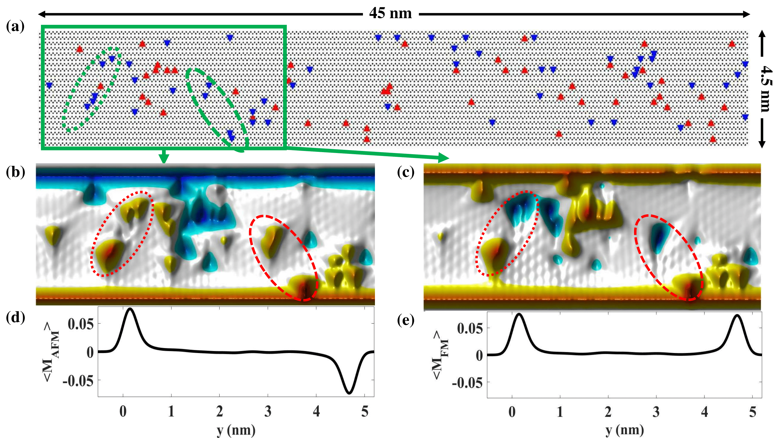
Figure 1: (Color online) (a) Graphene nanoribbon lattice structure with 10010 atoms and randomly generated 1% defects concentration equally distributed within A-sublattice (downward pointed triangles) and B-sublattice (upward pointing triangles). (b) AFM (ground state) and (c) FM spin denstiy profile of a portion of the ribbon. (d) and (e) Average magnetization along the ribbon length for the AFM and FM phases.

The first term is for the tight-binding (TB) approximation where the $t_{ij}$ are the hopping parameters are taken to be $t_{nn}$= -2.8 eV for the nearest neighbours and $t_{nnn}$= -0.1 eV for the second nearest neighborsNeto+09 ; Reich+02 . The creation $c^{\dagger}_{i\sigma}$ and $c_{i\sigma}$ annihilation operators create and annihilate an electron at the ith orbital with spin $\sigma$, respectively. The terms $\operatorname{}\langle n_{i\sigma}\rangle$ correspond to the expectation value of electron densities. The second and third terms are on-site and long-range Coulomb interaction terms, respectively. The on-site Coulomb potential $U$ is taken to be $16.522/\kappa$ eV, where $\kappa=6$ is an effective dielectric constant. The long-range interaction parameters $V_{ij}$ are taken to be $8.64/\kappa$ eV and $5.33/\kappa$ eV for the first two neighbours, and $1/d_{ij}\kappa$ for distant neighborsSlatermatrix . However, unlike for ZGNRs in the presence of long range disorderUlas+16 , the effect of long-range Coulomb interactions is found to be negligible in the presence of atomic defects considered in current work.

We consider 45 nm long and 4.5 nm wide ZGNRs consisting of 10010 atoms with various defect configurations. Figure 1a shows a ZGNR configuration with 1% of defects that are randomly and equally distributed among the two sublattices of the honeycomb lattice. The downward pointing (blue color online) and upward pointing (red color online) triangles correspond to sublattice A-site and B-site vacancies, respectively. The self-consistent Hubbard calculations were performed within different $S_{z}$=($n_{\uparrow}$ - $n_{\downarrow}$)/2 subspaces to find the overall ground state. As one may suspect a competition between the AFM and FM statesUlas+16 , we have scanned the $0$ $\leq$ $S_{z}$ $\leq$ $130$ values, with a focus around AFM state $S_{z}$=0 and FM state $S_{z}=N_{edge}/2$ where the number of edge states is given by $N_{edge}=138$ for the clean structure. For each value $S_{z}$ the self consistent calculations were repeated with different initial density matrices to ensure the convergence to the global energy minimum.

Figures 1b and 1c shows the spin densities of a portion of the ribbon, for the lowest energy AFM and FM states, respectively. Despite the inclusion of long range electron interactions and second nearest neighbour hoppings, the mean-field solution to the Hubbard model leads to $S_{z}=0$ ground state in all our calculations with equally distributed defects among the two sublattices, in agreement with Lieb’s theorem. Indeed, in Fig.1b, the A-site and B-site defects lead to spin-up (red color online) and spin-down (blue color online) magnetic moments, respectively, as expected. On the other hand, the spin density distribution for the lowest FM state is harder to predict since it is not a ground state consistent with Lieb’s theorem. Interestingly, the edge ferromagnetism of the $S_{z}=73$ state remains robust (see Fig.1c) and the bulk atoms have a zero average magnetization as shown in Fig.1d-e. This simple observation has an important consequence on the stability of the AFM phase with respect to the FM phase: For the FM phase, the magnetization of the defects nearby edge atoms is strictly dictated by the strong magnetization of the edges, locally obeying Lieb’s theorem. Hence, far from the edges, one must encounter sublattice spin frustrations where Lieb’s theorem cannot be locally satisfied, costing energy. For instance, for the AFM state where the Lieb’s theorem is globally satisfied, the A-site defects in the encircled areas in Figs.1b are ferromagnetically coupled to each other, whereas their coupling is antiferromagnetic in Fig.1c. Our calculations show that such local violation of Lieb’s theorem only occurs among defect sites and never between an edge and a defect site.

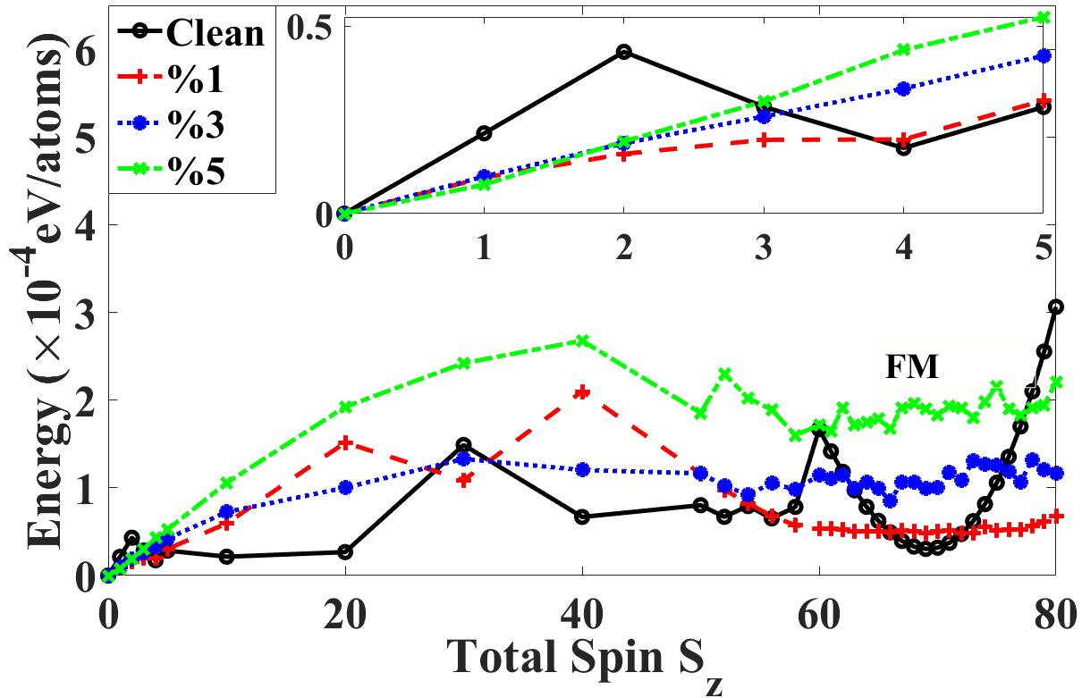
Figure 2: (Color online) Mean-field energy per atom as a function of total spin $S_{z}$ for clean, 1%, 3%, and 5% of defect concentrations. For the clean case, the ground state is AFM edges with $S_{z}$=0, and the FM phase occurs at $S_{z}$=69. The FM-AFM gap increases with increasing defects concentration.

As discussed above, local violation of Lieb’s theorem in the bulk region of the FM phase costs energy. A striking consequence of the energy cost is an increased stability of the AFM phase with respect to the FM phase. Figure 2 shows the energy per atom of different magnetic states $S_{z}$ with respect to the AFM ground state, for various defect concentrations up to $5\%$. For clean structure, the FM phase is at $S_{z}=N_{edge}/2=69$ and the FM-AFM gap is $3.041\times 10^{-5}$ eV/atom. As the defect concentration is increased, the FM-AFM gap increases, reaching $1.6\times 10^{-4}$ eV for the 5% of defects. Strikingly, the gap increase with respect to the AFM phase occurs not only for FM phase but most other $S_{z}$ states. However, in the vicinity of $S_{z}=0$ (see the inset), i.e. for single/few spin flips, energy cost is decreased at $1\%$ of defect concentrations, but then increases slightly with increasing number of defects. This reflects the fact that for low defect concentrations it is easier to flip an edge spin by moving it into a defect state than into the opposite edge. We note that similar behaviors were observed for other randomly generated defect concentrations and a statistical analysis will be presented below in Fig.4.

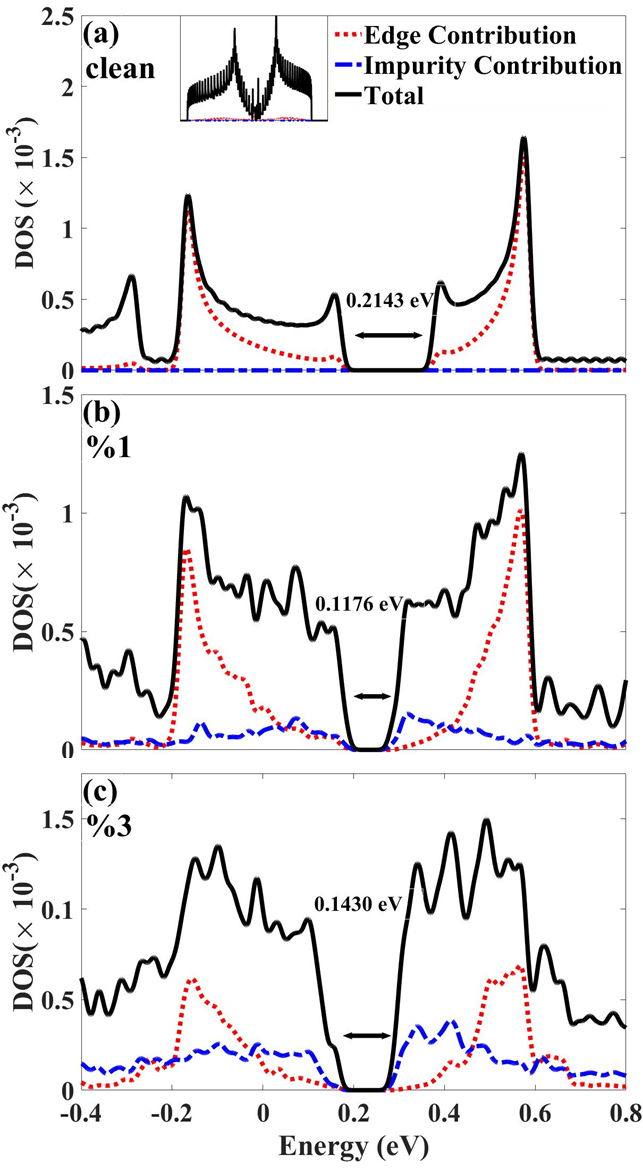
Figure 3: (Color online) Mean-field DOS for the AFM phase for the (a) clean, (b) 1% concentration, and (c) 3% concentration cases. Edge and defect states contributions are plotted with dotted and dot-dashed lines. Energy gap values of the total DOS are given for each case.

Figure 3 shows the mean-field density of states (DOS) for AFM ground state, for different concentrations considered in Fig.2. The solid lines represent the total DOS, whereas the dotted and dashed lines represent the contribution from edge and defect atoms (more precisely, atoms neighbouring the defects/vacancies) to the DOS, respectively. For the clean nanoribbon, the AFM gap is 0.2143 eV, which roughly corresponds to the energy required to flip a single spin. As the defect concentration is increased to 1%, there is an increase of midgap state density and the AFM gap is decreased to 0.1176 eV. This is consistent with the single spin flips in the vicinity of $S_{z}=0$ discussed in Fig.2. When the concentration of defects is increased to 3%, the AFM gap now increases slightly. This change of behavior reflects the fact that for higher number of defects the magnetic coupling between the defects is enhanced in average, stabilizing the magnetic configuration and making the spin flips harder. However, we note that, the AFM-FM gap monotonically increases with increasing midgap states due to the local violation of Lieb’s theorem, as discussed earlier.

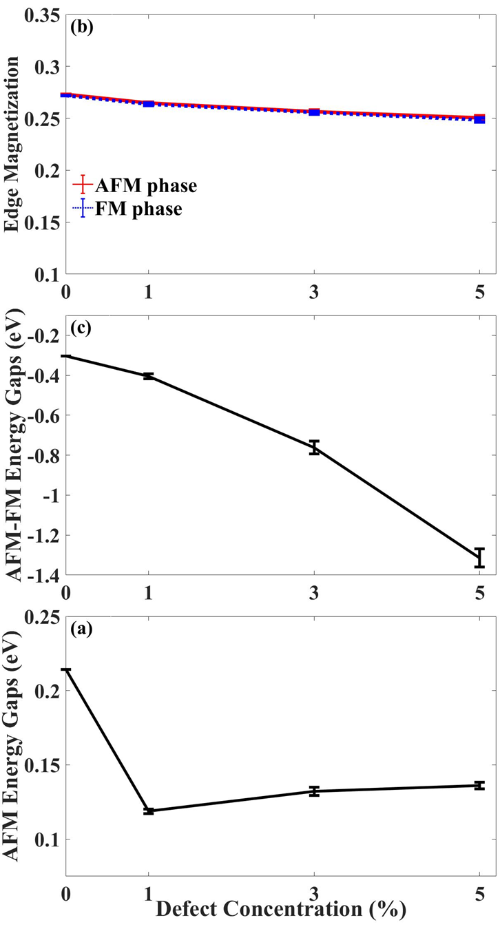
Figure 4: (Color online) Average (a) single edge magnetization,(b) AFM-FM energy gap, and (c) AFM energy gap, over 10 randomly generated disorder configurations, as a function of defect concentration.

Up to this point, the results presented were obtained for particular randomly generated defect configurations. For a statistical analysis of our results, we have repeated our calculations for 10 randomly generated configuration at 1, 3, and 5% defect concentrations. We have observed similar behavior in all the disorder configurations and the results are presented in Fig.4 as a function of defect concentration. The average magnetization of edge atoms for the AFM and FM phases, shown in Fig.4a, decreases slightly with increasing defect concentration. The difference between the AFM and FM edge magnetization remains negligible (within the error bars), consistent with Figs.1d-e. On the other hand, Fig. 4b shows that the AFM-FM gap rapidly decreases in average with a small error bar, clearly demonstrating an increased stability of the AFM phase with respect to the FM phase. Finally, the average AFM gap shown in Fig.4c, indicating the energy cost for a single spin flip, systematically undergoes a decrease at lower concentrations, then keeps slowly increasing at concentrations higher than 1% due to a more stable magnetic lattice formed by defects.

In summary, effects of randomly distributed atomic defects on the stability of magnetic phases of a zigzag edged graphene nanoribbon were investigated using a mean-field Hubbard approach. For an equal distribution of atomic defects among the two sublattices of the honeycomb lattice, the ground state remains antiferromagnetic with $S_{z}=0$. At lower defect concentrations ( $\leq 1\%$ ), the energy of single spin flips from the antiferromagnetic ground state is decreased due to possible electron transfer from edges to defect states. However, we show that the AFM-FM energy gap remains well protected and is enhanced as a function defect concentration. The increased stability of the AFM-FM gap by controlling defect concentrations opens up new possibilities for spintronic and magnetic nanodevice applications.

Acknowledgment. This work was supported by The Scientific and Technological Research Council of Turkey (TUBITAK) under the 1001 Grant Project No. 114F331. The numerical calculations reported in this work were partially performed at TUBITAK ULAKBIM, High Performance and Grid Computing Center (TRUBA resources).

References

- (1) D. D. Awschalom, L. C. Bassett, A. S. Dzurak, E. L. Hu, and J. R. Petta, Science , 339, 1174 (2013).
- (2) S. A. Wolf et al., Science 294, 1488 (2001)
- (3) C. Chappert, A. Fert, and F. N. Van Dau, Nature Mater. 6, 813 (2007)
- (4) Y.W.Son, M. L. Cohen, and S. G. Louie, Nature (London), 444, 347 (2006)
- (5) Wei L. Wang, Oleg V. Yazyev, Sheng Meng, and Efthimios Kaxiras Phys. Rev. Lett. , 102 157201 (2009)
- (6) J. Fernández-Rossier and J. J. Palacios Phys. Rev. Lett. 99, 177204 (2007).
- (7) O. V.Yazyev and M. I. Katsnelson, Phys. Rev. Lett., 100, 047209 (2008)
- (8) Michael Wimmer, İ. Adagideli, Savaş Berber, David Tománek, and Klaus Richter, Phys. Rev. Lett. 100, 177207 (2008).
- (9) B. Trauzettel, D. V. Bulaev, D. Loss, and G. Burkard, Nat. Phys. 3, 192 (2007)
- (10) A. D. Güçlü, P. Potasz, and P. Hawrylak, Phys. Status Solidi,RRL 10, 1, 58-67 (2015).
- (11) A. D. Güçlü, P. Potasz, O. Voznyy, M. Korkusinski, and P. Hawrylak, Phys. Rev. Lett 103, 246805 (2009)
- (12) Elliott H. Lieb, Phys. Rev. Lett. 62, 1201 (1989)
- (13) M. Fujita, K. Wakabayashi, K. Nakada, and K. Kusakabe, J. Phys. Soc. Jpn. 65, 1920 (1996).
- (14) Hosik Lee, Y.W. Son, Noejung Park, Seungwu Han, and Jaejun Yu Phys. Rev. B 72, 174431 (2005).
- (15) Y.W. Son, M.L. Cohen, and S.G. Louie, Phys. Rev. Lett. 97, 216803 (2006).
- (16) T. C. Li and Shao-Ping Lu Phys. Rev. B , 77, 085408 (2008).
- (17) F. Cervantes-Sodi, G. Csányi, S. Piscanec, and A. C. Ferrari Phys. Rev. B , 77,165427 (2008).
- (18) Tobias Wassmann, Ari P. Seitsonen, A. Marco Saitta, Michele Lazzeri, and Francesco Mauri, Phys. Rev. Lett. 101, 096402 (2008)
- (19) A. D. Güçlü, P. Potasz, and P. Hawrylak, Phys. Rev. B 88, 155429 (2013)
- (20) H.U. Özdemir, A.Altıntaş, and A.D.Güçlü Phys. Rev. B , 93 014415 (2016)
- (21) H. Şahin,R. T. Senger, and S. Ciraci, Journal of appl. phys. 108, 074301 (2010)
- (22) Oleg V Yazyev, Science 73, 5 (2010)
- (23) J. Jung and A. H. MacDonald, Phys. Rev. B 79, 235433 (2009)
- (24) P. Potasz, A. D. Güçlü, A. Wójs,and P. Hawrylak, Phys. Rev. B 81, 033403 (2010)
- (25) H. Feldner, Z.Y. Meng, A. Honecker, D. Cabra, S. Wessel, and F.F. Assaad Phys. Rev. B, 81, 115416 (2010).
- (26) G. Z. Magda, X. Jin , I. Hagymási, P. Vancsó, Z. Osváth, P. Nemes-Incze, C. Hwang, L. P. Biró, L. Tapasztó, Nature 514, 608 (2014)
- (27) M. Modarresi and A.D. Güçlü Phys. Rev. B 95, 235103 (2017)
- (28) Oleg V. Yazyev and Lothar Helm Phys. Rev. B , 75 125408 (2007)
- (29) J. J. Palacios, J. Fernández-Rossier, and L. Brey Phys. Rev. B , 77 195428 (2008)
- (30) W. Jaskolski, Leonor Chico, and A. Ayuela Phys. Rev. B , 91 165427 (2015)
- (31) H.Gonzalez-Herrero, J.M. Gomez-Rodriguez, P.Mallet, M. Moaied, J.J. Palacios, C.Salgado, M.M. Ugeda, J.Y. Veuillen, F.Yndurain, and I. Brihuega, Science 352, 437 (2016)
- (32) Fernando Gargiulo, Gabriel Autés, Naunidh Virk, Stefan Barthel, Malte Rösner, Lisa R. M. Toller, Tim O. Wehling, and Oleg V. Yazyev Phys. Rev. Lett. , 113, 246601 (2014).
- (33) P. Esquinazi, D. Spemann, R. Höhne, A. Setzer, K.-H. Han, and T. Butz Phys. Rev. Lett. 91, 227201 (2003).
- (34) D. Soriano, F. Munoz-Rojas, J. Fernández-Rossier, and J. J. Palacios Phys. Rev. B , 81, 165409 (2010)
- (35) Singh R., Kroll P. J Phys Condens Matter. , 21(19):196002 (2009)
- (36) A.D. Güçlü, N. Bulut Phys. Rev. B 91, 125403 (2015).
- (37) Yu Zhang, Si-Yu Li, Huaqing Huang, Wen-Tian Li, Jia-Bin Qiao, Wen-Xiao Wang, Long-Jing Yin, Ke-Ke Bai, Wenhui Duan, and Lin He, Phys. Rev. Lett. 117, 166801 (2016).
- (38) Oleg V. Yazyev Phys. Rev. Lett. 101, 037203 (2008).
- (39) Vitor M. Pereira, F. Guinea, J.M.B. Lopes dos Santos, N.M.R. Peres, and A.H. Castro Neto Phys. Rev. Lett. 96, 036801 (2006).
- (40) Leopold Talirz, Hajo Söde, Tim Dumslaff, Shiyong Wang, Juan Ramon Sanchez-Valencia, Jia Liu, Prashant Shinde, Carlo A. Pignedoli, Liangbo Liang, Vincent Meunier, Nicholas C. Plumb, Ming Shi, Xinliang Feng, Akimitsu Narita, Klaus Müllen, Roman Fasel, and Pascal Ruffieux, ACS Nano, 11, 1380-1388 (2017)
- (41) Giang D. Nguyen, Hsin-Zon Tsai, Arash A. Omrani, Tomas Marangoni, Meng Wu, Daniel J. Rizzo, Griffin F. Rodgers, Ryan R. Cloke, Rebecca A. Durr, Yuki Sakai, Franklin Liou, Andrew S. Aikawa, James R. Chelikowsky, Steven G. Louie, Felix R. Fischer,and Michael F. Crommie, Nature Nanotechnology, 12, 1077-1082 (2017)
- (42) Michael C. Chong, Nasima Afshar-Imani, Fabrice Scheurer, Claudia Cardoso, Andrea Ferretti, Deborah Prezzi, and Guillaume Schull, Nano Lett., 18, 175-181 (2018)
- (43) Dimas G. de Oteyza, Aran Garcia-Lekue, Manuel Vilas-Varela, Néstor Merino-Diez, Eduard Carbonell-Sanromá, Martina Corso, Guillaume Vasseur, Celia Rogero, Enrique Guitián, Jose Ignacio Pascual, J. Enrique Ortega, Yutaka Wakayama, and Diego Peña, ACS Nano, 10(9), 9000-9008 (2016)
- (44) Hironobu Hayashi , Junichi Yamaguchi, Hideyuki Jippo, Ryunosuke Hayashi, Naoki Aratani , Mari Ohfuchi, Shintaro Sato, and Hiroko Yamada, ACS Nano, 11(6), 6204-6210 (2017)
- (45) Robert M. Jacobberger and Michael S. Arnold, ACS Nano, 11(9), 8924-8929 (2017)
- (46) Robert S. Jordan , Yolanda L. Li, Cheng-Wei Lin, Ryan D. McCurdy, Janice B. Lin , Jonathan L. Brosmer , Kristofer L. Marsh, Saeed I. Khan, K. N. Houk , Richard B. Kaner , and Yves Rubin, J. Am. Chem. Soc., 139(44), 15878-15890 (2017)
- (47) Ayrat M. Dimiev, Artur Khannanov, Iskander Vakhitov, Airat Kiiamov, Ksenia Shukhina, and James M. Tour, ACS Nano, , Article ASAP (2018)
- (48) Nataliya Kalashnyk, Kawtar Mouhat, Jihun Oh, Jaehoon Jung, Yangchun Xie, Eric Salomon, Thierry Angot, Frédéric Dumur, Didier Gigmes and Sylvain Clair, Nature Comm., 8, 14735 (2017)
- (49) Lingxiu Chen, Li He, Hui Shan Wang, Haomin Wang, Shujie Tang, Chunxiao Cong, Hong Xie, Lei Li, Hui Xia, Tianxin Li, Tianru Wu, Daoli Zhang, Lianwen Deng, Ting Yu, Xiaoming Xie and Mianheng Jiang, Nature Comm., 8, 14703 (2017)
- (50) P. H. Jacobse, A. Kimouche, T. Gebraad, M. M. Ervasti, J. M. Thijssen, P. Liljeroth and I. Swart, Nature Comm., 8, 119 (2017)
- (51) Gerald Schubert and Holger Fehske, Phys. Rev. Lett. 108, 066402 (2012)
- (52) M. Topsakal, E. Aktürk, H. Sevinçli, and S. Ciraci, Phys. Rev. B. 78, 235435 (2008)
- (53) Q. Q. Dai, Y. F. Zhu, and Q. Jiang, Journal of phys. chem. C 117, 4791-4799 (2013)
- (54) A.H.C.Neto, F.Guinea, N.M.R. Peres, K.S. Novoselov, and A. K. Geim, Rev. Mod. Phys. 81 109 (2009)
- (55) S. Reich, J. Maultzsch, C. Thomsen, and P. Ordejón Phys. Rev. B 66 035412 (2002)
- (56) P. Potasz, A. D. Güçlü, and P. Hawrylak Phys. Rev. B 82 075425 (2010)