Online Convex Optimization and No-Regret Learning:
Algorithms, Guarantees and Applications

Abstract.

Spurred by the enthusiasm surrounding the “Big Data” paradigm, the mathematical and algorithmic tools of online optimization have found widespread use in problems where the trade-off between data exploration and exploitation plays a predominant role. This trade-off is of particular importance to several branches and applications of signal processing, such as data mining, statistical inference, multimedia indexing and wireless communications (to name but a few). With this in mind, the aim of this tutorial paper is to provide a gentle introduction to online optimization and learning algorithms that are asymptotically optimal in hindsight – i.e., they approach the performance of a virtual algorithm with unlimited computational power and full knowledge of the future, a property known as no-regret. Particular attention is devoted to identifying the algorithms’ theoretical performance guarantees and to establish links with classic optimization paradigms (both static and stochastic). To allow a better understanding of this toolbox, we provide several examples throughout the tutorial ranging from metric learning to wireless resource allocation problems.

1. Introduction

The prototypical setting of online optimization is as follows: at each stage of a repeated decision process, an optimizing agent makes a prediction and incurs a loss based on an a priori unknown cost function that measures the accuracy of said prediction. Subsequently, the agent receives some problem-specific feedback and makes a new prediction, possibly against a different ground truth (empirical evidence), with the goal of improving the quality of their predictions over time. In this broad context, the theory of online optimization seeks to characterize the limits of what is achievable in terms of performance guarantees, and to provide efficient algorithms to achieve them.

Spurred by the enthusiasm surrounding the Big Data paradigm, the mathematical and algorithmic tools developed in the field of online optimization have found widespread use in problems where the trade-off between data exploration and exploitation plays a predominant role. In signal processing, examples of this include sparse coding and dictionary learning [29], data classification and filtering [18], matrix completion and prediction [47], and many others. More recently, motivated by the highly dynamic nature of future and emerging wireless networks, online optimization methods have been successfully exploited to design resource allocation policies for problems ranging from signal covariance optimization in multi-antenna terminals [32] to channel selection and cognitive medium access [4].

In classic, static optimization problems, the core underlying assumption is that the objective to be optimized is known by the optimizing agent and remains fixed for the entire runtime of the algorithm computing a solution. Stochastic optimization provides an extension of this framework to problems where the objective function may also depend on a stationary stochastic process. Game theory takes an alternative, multi-agent view of such problems, often revolving around worst-case guarantees against an adversary – e.g., as in von Neumann’s celebrated minimax vision of zero-sum games. However, all these extensions rely on strong assumptions regarding the variability of the problem’s objective, the agents’ rationality and common knowledge of rationality (in games), the information at the agents’ disposal, etc. By contrast, online optimization provides an elegant toolbox which goes beyond the above by allowing for variations in the problem that are completely arbitrary – typically accounting for exogenous (stationary or otherwise) parameters affecting it (cf. Fig. 1).

Figure 1. A bird’s eye view of the links between online optimization and other optimization paradigms.

A key example of this framework is encountered in wireless communication networks, where traditional static/stationary paradigms no longer suffice to capture and cope with issues such as non-random fluctuations in the wireless medium, the unpredictable behavior of the communicating devices in distributed networks, etc. [31, 32]. Likewise, in metric learning problems for multimedia indexing and classification, the online framework allows to exploit distributed annotations from multiple input sources (such as the Internet users), as opposed to relying on centralized annotation of very large data sets, and also to relax all the stochastic assumptions among annotations that are common in offline metric learning [26].

In addition to its wide-ranging scope, another major advantage of the online framework is that the derived algorithms – referred here as online policies – come with provable theoretical guarantees in the face of uncertainty. These guarantees are based on Hannan’s definition of regret [22], a seminal notion which compares an algorithm’s performance to that of the best fixed policy in hindsight, an idealized benchmark that minimizes the total loss incurred over the horizon of play with perfect knowledge of the future. Since this benchmark requires full, non-causal knowledge of the dynamics governing the evolution of the problem’s objective, this is obviously not an implementable policy – it only exists as a theoretical performance target. As such, the aim of online optimization is to derive causal, online learning algorithms that get as close as possible to this formidable target with the fewest possible assumptions. What is truly striking is that it succeeds: the last two decades have seen a flurry of activity on the design of online algorithms that attain the best possible regret minimization rates in a broad range of problems, thus explaining the widespread use of such algorithms in Big Data.

We dive in all this by first exploring in Section 2 a fundamental discrete choice problem that has been the focus of a very active and vigorous literature: multi-armed bandits (MABs). This problem is simple to state and provides a gentle introduction to the fundamental exploration–exploitation trade-off that underlies much of online optimization; at the same time, it is sufficiently deep to require highly sophisticated analytical tools to solve it. A key lesson from this problem is that deterministic online policies suffice to achieve no regret in (stationary) stochastic environments. However, when pitted against an informed adversary, such algorithms are doomed to fail: when “gambling in a rigged casino”, only randomized algorithms can surprise the adversary often enough to attain a no-regret state.

Extending the above to problems with continuous action spaces, we introduce in Section 3 the fundamentals of online optimization (along with several applications and examples), and we discuss in Section 4 the most widely studied classes of online algorithms and their theoretical guarantees (again, with several practical applications). Specifically, we focus on Zinkevich’s seminal online gradient descent (OGD) method [50] and on its generalization: the class of online mirror descent (OMD) schemes pioneered by Shalev-Shwartz [44, 45]. By tailoring each method to the geometry of the problem at hand, it is possible to attain regret minimization rates that are provably optimal in terms of the problem’s dimension, going as far as achieving a logarithmic reduction thereof. This is a powerful instance of lifting the curse of dimensionality: in many machine learning and Big Data applications, the dimension of the problem’s state space is exponentially large, so these techniques render the solution of such problems feasible. Finally, we discuss in Section 5 the impact of noise and imperfections in the feedback received by the optimizer, the possibility to learn without gradient-based feedback, and other considerations that arise in practice.

To sum up, this tutorial is intended for researchers and graduate students interested in an overview of online optimization and no-regret learning, including theoretical guarantees, the algorithms that achieve them, and their applications. More specifically, our goal is to:

• Provide a holistic overview of the topic highlighting its connections with other optimization paradigms.

• Delineate the fundamental theoretical limits of what can be achieved and present the algorithms that achieve these limits.

• Explain to what extent the feedback limitations that arise in practical signal processing applications affect the performance of such algorithms.

• Provide applications and examples from different areas of signal processing to help the reader appreciate the wide applicability of online optimization and no-regret learning methods.

Our goal is to give an introduction to these questions, without going into overwhelming detail. In particular, we make no effort or claim of providing a comprehensive survey of the state-of-the-art; this would require a much more in-depth treatment than an introductory tutorial is meant to provide, so we do not attempt it.

Landau notation

Throughout this tutorial, we will make heavy use of the Landau asymptotic notation $\operatorname{\mathcal{O}}(\cdot)$, $o(\cdot)$, $\Omega(\cdot)$, etc. First, given two functions $f,g\colon\mathbb{R}\to\mathbb{R}$, we say that “$f$ grows no faster than $g$ asymptotically” and we write $f(t)=\operatorname{\mathcal{O}}(g(t))$ as $t\to\infty$ if $\limsup_{t\to\infty}f(t)/g(t)<\infty$, i.e., there exists some positive constant $c>0$ such that $\lvert f(t)\rvert<g(t)$ for sufficiently large $t$. Conversely, we say that “$f$ grows no slower than $g$” and we write $f(t)=\Omega(g(t))$ if $g(t)=\operatorname{\mathcal{O}}(f(t))$ or, equivalently, $\limsup_{t\to\infty}g(t)/f(t)>0$. If we have both $f(t)=\operatorname{\mathcal{O}}(g(t))$ and $f(t)=\Omega(g(t))$, we say that “$f$ grows as $g$” and we write $f(t)=\Theta(g(t))$. Finally, if $\limsup_{t\to\infty}f(t)/g(t)\leq 0$, we write $f(t)=o(g(t))$ and we say that “$f$ is dominated by $g$” (we ignore the negative part).

2. A Gentle Start: Multi-Armed Bandits

We begin with the multi-armed bandit (MAB) problem, a fundamental sequence prediction (or forecasting) problem that permeates many areas of online and machine learning, and which has found a remarkable breadth of applications – from sparse coding and dictionary learning [29], to filtering [18], matrix prediction [47], channel selection [4], antenna beam selection in mmWave communications [23] and many others. In a certain sense, multi-armed bandits comprise the “discrete” analogue of the more general online optimization framework that we treat in the rest of this monograph. We begin with this case mostly for historical reasons – but also to illustrate some of the key notions involved, which is easier to do in the multi-armed bandit (MAB) setting.

After a brief overview, we introduce the notion of regret in the context of stochastic multi-armed bandits and we present the upper confidence bound (UCB) algorithm, a deterministic policy that achieves no regret in this problem. Beyond stochastic bandits, when facing an adversary (sometimes referred to as “gambling in a rigged casino”), deterministic policies are no longer able to attain a no-regret state, so we turn to randomized strategies and present the regret guarantees of the exponential weights (EW) algorithm, with both full and partial information.

2.1. Problem Statement

Dating back to the seminal work of Thompson [49] and Robbins [40], a multi-armed bandit problem can be described as follows: At each stage $t=1,2,\dotsc$, of a repeated decision process, an optimizing agent (the decision-maker) selects an action $a_{t}$ from some finite set $\mathcal{A}=\{1,\dotsc,A\}$. Based on this choice, the agent receives a reward (or payoff) $u_{t}(a_{t})$, they select a new action $a_{t+1}$ and the process repeats. Sometimes it is more convenient to state the problem in terms of incurred losses instead of received payoffs; when this is the case, we will write $\ell_{t}(a_{t})=-u_{t}(a_{t})$ for the loss incurred by the agent at stage $t$.

Of course, the interpretation of the agents’ actions and their rewards (or losses) is context-specific and depends on the application at hand. In Robbins’ original formulation, the agent was a gambler choosing a slot machine in a casino (a “one-armed bandit” in the colorful slang of the 50’s), and the agent’s reward was the amount of money received minus the cost of playing [40]. In clinical trials (the setting of Thompson’s work), the choice of action represents the drug administered to a test patient and the incurred loss is the patient’s time to recovery [49]. A concrete example from wireless communications is as follows:

Example 2.1 (Channel selection).

Referring to [4] for the details, consider a wireless user transmitting over a set of $\mathcal{A}=\{1,\dotsc,A\}$ of non-overlapping frequency channels. At each time slot $t=1,2,\dotsc$, a channel $a\in\mathcal{A}$ could be either “free” or “busy”: if the chosen channel is free, the user’s packet is transmitted successfully, otherwise there is a collision and the packet is lost. Writing $v_{a,t}\in\{0,1\}$ for the state of channel $a$ at time $t$ (with $v_{a,t}=0$ indicating that the channel is free), the user’s loss at time $t$ is $\ell_{t}(a_{t})=-v_{a_{t},t}$, indicating a loss of $1$ whenever a packet drop occurs. Hence, to maximize throughput, the user’s objective is to minimize the total loss $\sum_{t=1}^{T}\ell_{t}(a_{t})$, i.e., the total number of packets dropped over the horizon $T$. Since the channel statistics change with the number of users in the system (and are typically unknown to the users anyway), the main challenge is to design channel selection algorithms that minimize this loss “on the fly”, i.e., as information becomes available over time.

Exploration vs. exploitation

Returning to the general bandit setting, it is easy to see that the optimizer faces a trade-off between exploration and exploitation. On the one hand, by trying out more arms (i.e., “exploring”), the agent obtains more information and can make better choices in the future. On the other hand, in so doing, the agent fails to take advantage of arms that yield better payoffs now, thus lagging behind in terms of performance (i.e., “exploitation”). As an example, in the channel selection problem, the more data used to train a scheduling algorithm, the better the channel selection will (eventually) become; however, this comes at the expense of false positives (or negatives) that severely hamper the user’s overall throughput. Achieving – and maintaining – a balance between exploration and exploitation is the main objective of the literature on multi-armed bandits.

Building on the above, there is a coarse categorization of multi-armed bandits based on the way the sequence of payoff functions $u_{t}\colon\mathcal{A}\to\mathbb{R}$ is generated. These are as follows:

1. Stochastic bandits: Each arm $a\in\mathcal{A}$ is associated to a statistical distribution $P_{a}$ and, at each stage $t=1,2,\dotsc$, the reward $u_{t}(a)$ of the $a$-th arm is an independent and identically distributed (i.i.d.) random variable $v_{a,t}$ drawn from $P_{a}$ (i.e., $u_{t}(a)\equiv v_{a,t}\sim P_{a}$ for all $a\in\mathcal{A}$ and all $t=1,2,\dotsc$). The arms’ reward distributions are not known to the agent, so the objective is to identify – and exploit – the arm with the highest mean reward in as few trials as possible.

2. Adversarial bandits: The payoff of each arm is determined by an “adversary” (real or fictitious) who prescribes the $t$-th stage “payoff vector” $v_{t}=(u_{t}(a))_{a\in\mathcal{A}}$ at the same time that the agent chooses an arm. In a certain sense, this is one of the most general formulations of the MAB problem as all distributional assumptions are removed. Thus, solving the adversarial problem also induces a solution to the stochastic bandit problem (though, perhaps, suboptimal).

3. Markovian bandits: The loss function $u_{t}$ is determined by the state $\omega_{t}$ of an underlying – and possibly hidden – Markov chain. The transition matrix of this Markov chain is a priori unknown, and the optimizer’s objective is to maximize their (discounted) expected reward over time.

In what follows, we describe the stochastic and adversarial MAB frameworks in detail. Albeit historically significant, the discounted reward and information structure of Markovian bandits makes them less suitable for signal processing applications, so they are not considered further in this tutorial; the interested reader can find a recent survey of the topic in [20].

2.2. Stochastic Bandits

In a stochastic multi-armed bandit, the agent’s objective would be to play the arm with the highest mean reward as many times as possible over the horizon of play $T$. To quantify this, let $\mu_{a}$ denote the mean value of the reward distribution $P_{a}$ of arm $a\in\mathcal{A}$ and let

$$\mu^{\ast}=\max_{a\in\mathcal{A}}\mu_{a}\quad\text{and}\quad a^{\ast}=\operatorname*{arg\,max}_{a\in\mathcal{A}}\mu_{a}$$ (2.1)

respectively denote the bandit’s maximal mean reward and the arm that achieves it (a priori, there could be several such arms but, for simplicity, we assume here that there is only one). A standard assumption is to further posit that the bandits’ rewards are always drawn from $[0,1]$: this is simply a normalization convention motivated by the Bernoulli bandit problem where each arm $a\in\mathcal{A}$ returns a payoff of $1$ with probability $p_{a}$ and $0$ with probability $1-p_{a}$.

2.2.1. Regret

With all this in mind, the agent’s performance after $T$ rounds can be quantified by aggregating the mean payoff gap between the bandit’s best arm and the arm $a_{t}$ chosen by the optimizer at each round $t=1,2,\dots,T$. This quantity is known as the agent’s mean regret and is formally defined as

$$\bar{R}_{T}=\sum_{t=1}^{T}\operatorname{\mathbb{E}}[u_{t}(a^{\ast})-u_{t}(a_{t})]=T\mu^{\ast}-\sum_{t=1}^{T}\operatorname{\mathbb{E}}[u_{t}(a_{t})].$$ (2.2)

For an alternative interpretation of $\bar{R}_{T}$, let $n_{a,t}$ denote the number of times that $a$ has been chosen up to time $t$ and write $\Delta_{a}=\mu^{\ast}-\mu_{a}$ for the mean payoff difference between arm $a$ and the bandit’s best arm. Then, an easy rearrangement of (2.2) yields the key expression

$$\bar{R}_{T}=\operatorname{\mathbb{E}}\left[\sum_{a\in\mathcal{A}}n_{a,T}\right]\,\mu^{\ast}-\operatorname{\mathbb{E}}\left[\sum_{a\in\mathcal{A}}\mu_{a}n_{a,T}\right]=\sum_{a\in\mathcal{A}}\Delta_{a}\operatorname{\mathbb{E}}[n_{a,T}].$$ (2.3)

Written this way, $\bar{R}_{T}$ can be viewed as the mean number of suboptimal choices made by the optimizer, weighted by the suboptimality gap $\Delta_{a}$ of each arm; put differently, $\bar{R}_{T}$ can be seen as a measure of the average number of mistakes made by the optimizer up to stage $T$.

In view of the above, maximizing the aggregate reward over $T$ stages of play amounts to asking the regret be sublinear in $T$. This is formally defined as

$$\bar{R}_{T}=o(T),$$ (2.4)

a property which is known as no regret and which guarantees that the relative number of mistakes (i.e., draws of suboptimal arms) must vanish in the long run. As a result, much of the literature on stochastic bandits has focused on the design of algorithms that attain the best possible regret minimization rate in (2.4).

2.2.2. No-regret algorithms for stochastic bandits

A straightforward idea to optimize one’s gains would be to keep a running average of the rewards obtained by each arm and then play the arm with the best estimate. This pure exploration (or “follow the leader”) policy can be formally described as

$$a_{t+1}=\operatorname*{arg\,max}_{a\in\mathcal{A}}\hat{\mu}_{a,t}$$ (2.5)

where

$$\hat{\mu}_{a,t}=\frac{1}{n_{a,t}}\sum_{s=1}^{t}\operatorname{\mathds{1}}(a_{s}=a)\,v_{a,s}$$ (2.6)

denotes the empirical mean payoff of arm $a$ (i.e., the total reward obtained from arm $a$ normalized by the number of times it was drawn). This policy is a reasonable first try but it can easily get stuck at a suboptimal arm: if the best arm performs very badly in its first draws, “following the leader” means it won’t be drawn again in the future, so the agent’s regret will grow linearly over time.

The above highlights the need for adding at least some exploration into the mix: otherwise, pure exploitation cannot lead to sublinear regret. Building on this observation, the landmark idea of [28, 6] was to retain optimism in the face of uncertainty, i.e., to construct an “optimistic” estimate for the mean payoff of each arm, and then pick the arm with the highest such estimate. If this guess is wrong, optimism will fade quickly; but if the guess is right, the agent will be able to balance exploration and exploitation, incurring little regret in the process.

The key ingredient of this “optimism” principle is provided by Hoeffding’s inequality, a fundamental tail bound in statistics which states that the sample mean $\bar{X}_{n}=n^{-1}\sum\nolimits_{i=1}^{n}X_{i}$ of a sequence of i.i.d. random variables $X_{i}\in[0,1]$ with mean $\mu$ satisfies

$$\operatorname{\mathbb{P}}\left(\bar{X}_{n}<\mu-z\right)\leq e^{-2nz^{2}}.$$ (2.7)

In our bandit setting, if we take $z=\sqrt{\alpha\log t/(2n_{a,t})}$ for some $\alpha>0$, it follows that

$$\operatorname{\mathbb{P}}\left(\hat{\mu}_{a,t}+\sqrt{\alpha\log t/(2n_{a,t})}<\mu_{a}\right)\leq t^{-\alpha},$$ (2.8)

i.e., the probability that the optimistic estimate $\hat{\mu}_{a,t}+\sqrt{\alpha\log t/(2n_{a,t})}$ is less than $\mu_{a}$ decays very fast as a function of $t$.

Algorithm 1 upper confidence bound (UCB) with parameter $\alpha$

0:  tuning parameter $\alpha>2$, initial reward sample $\hat{\mu}_{a}$ from each arm $a\in\mathcal{A}$

1:  set $n_{a}=1$ for all $a\in\mathcal{A}$ # initialization

2:  for $t=1$ to $T$ do

3:     draw $a_{t}\in\operatorname*{arg\,max}_{a\in\mathcal{A}}\left\{\hat{\mu}_{a}+\sqrt{\alpha\log t/(2n_{a})}\right\}$ # arm selection

4:     gain $\hat{u}_{t}=v_{a_{t},t}$ # receive reward

5:     $n_{a_{t}}\leftarrow n_{a_{t}}+1$ # sample size update

6:     $\hat{\mu}_{a_{t}}\leftarrow\left(1-\frac{1}{n_{a_{t}}}\right)\,\hat{\mu}_{a_{t}}+\frac{1}{n_{a_{t}}}\hat{u}_{t}$ # empirical mean update

7:  end for

Motivated by this, the upper confidence bound (UCB) algorithm with tuning parameter $\alpha>2$ is defined via the recursion

$$a_{t+1}=\operatorname*{arg\,max}_{a\in\mathcal{A}}\left\{\hat{\mu}_{a,t}+\sqrt{\frac{\alpha\log t}{2n_{a,t}}}\right\}.$$ (2.9)

Heuristically, the first term in (2.9) drives the agent to exploit the arm with the highest empirical mean while the second one encourages exploration by giving a second chance to arms which have not been played often enough (i.e., $n_{a,t}$ is small relative to $t$). This idea dates back to the landmark paper of Lai and Robbins [28] and was subsequently expanded by Agrawal [3], Auer et al. [6], and many others. For the specific variant considered here, the analysis of [13] gives:

Theorem 2.1 (UCB algorithm for stochastic bandits).

The UCB algorithm with parameter $\alpha>2$ enjoys the worst-case guarantee

$$\bar{R}_{T}\leq\sum_{a\neq a^{\ast}}\left(\frac{2\alpha}{\Delta_{a}}\log T+\frac{\alpha}{\alpha-2}\right)=\operatorname{\mathcal{O}}(\log T).$$ (2.10)

Importantly, the regret guarantee of UCB is optimal in $T$: the information-theoretic analysis of Lai and Robbins shows that no causal policy played against a bandit with Bernoulli reward distributions can achieve regret lower than $\Omega(\log T)$ [28]. Eliminating the gap between the multiplicative constants that appear in (2.10) and the Lai–Robbins lower bound has given rise to a significant body of literature: we only mention here the recent KL–UCB variant of [19] which essentially attains the Lai–Robbins bound and strictly dominates (2.9) for any class of bounded reward distributions. Further refinements under different assumptions are also possible, and we refer the reader to [13] for an introduction to this rich literature. Other than that however, in an application-agnostic setting, UCB provides a fairly complete solution to the stochastic MAB problem.

2.3. Adversarial Bandits

Stochastic bandits have found a wide range of applications in problems with a clear statistical character such as filtering [18], sequence prediction [15], etc. However, when the problem at hand is not purely statistical in nature (or when its statistics are influenced by exogenous, contextual factors), it is no longer possible to identify an “optimal” arm. In the context of signal processing, this is particularly important in communication problems that involve (slow) fading or jamming-proof coding [32], generative neural networks for image processing [21], game-theoretic applications [36], etc.

Tracing its roots to the “rigged casino” problem of [7], this paradigm is known as adversarial because the agent is called to learn against any possible sequence of rewards, including those designed by a mechanism that actively tries to minimize the agent’s cumulative payoff over time – an adversary. More precisely, at each step in an adversarial bandit problem, the rewards $u_{t}(a)$ of each arm $a\in\mathcal{A}$ are determined by the adversary simultaneously with the agent’s action $a_{t}$, possibly with full knowledge of the decision process employed by the agent at step $t$. Thus, optimizing in hindsight over the horizon of play, the agent’s realized regret is now defined as

$$R_{T}=\max_{a\in\mathcal{A}}\sum_{t=1}^{T}[u_{t}(a)-u_{t}(a_{t})],$$ (2.11)

i.e., as the cumulative payoff difference between the agent’s chosen arm and the best possible arm over the given horizon of play.

2.3.1. Adversarial vs. stochastic bandits

In an adversarial setting, the agent’s objective is to incur sublinear regret $R_{T}=o(T)$ against any sequence of rewards chosen by the adversary. However, in contrast to the stochastic case, this definition is not inherently probabilistic and does not include any (stochastic) averaging. In particular, if i ) the agent’s choice of arm is made by a deterministic algorithm that takes as input the history of play up to the current stage; and ii ) the adversary knows this algorithm in advance and uses it to design the worst possible sequence of outcomes, the sequence of play and the generated rewards are all deterministic.

This simple example shows that the stochastic and adversarial bandit paradigms are not immediately comparable. More importantly, it also illustrates Cover’s impossibility result [16]: a deterministic algorithm cannot hope to achieve sublinear regret against an adversarial bandit. Indeed, if the optimizer uses a deterministic algorithm which is known to the adversary, the adversary could set the reward $u_{s}(a_{s})$ of the optimizer’s chosen arm $a_{s}$ to $0$, and the rewards of all other arms $a\neq a_{s}$ to $1$. In so doing, after $T$ stages, the agent will have gained a cumulative payoff of $0$; however, any arm $a\in\mathcal{A}$ which has been chosen no more than $T/2$ times would have generated a cumulative payoff of at least $T/2$. The incurred regret is therefore $R_{T}\geq T/2$, showing that the agent cannot achieve sublinear regret in this setting.

Cover’s result shatters all hopes of minimizing regret with a deterministic algorithm in an adversarial setting. However, if the choice of the arms is randomized, different results may hold against an adversary. By this token, a meaningful relaxation of the problem is to allow for randomized arm selection: in this case, the agent is choosing an action $a_{t}$ at stage $t$ based on a probability distribution (or mixed strategy) $x_{t}=(x_{a,t})_{a\in\mathcal{A}}$ which assigns probability $x_{a,t}$ to arm $a$. The near-omniscient adversary might be fully aware of the agent’s mixed strategy at stage $t$, but the actual results of these randomized draws are not known in advance – otherwise, Cover’s impossibility result would still apply. The agent’s mean regret is then defined as

$$\bar{R}_{T}=\max_{a\in\mathcal{A}}\sum_{t=1}^{T}\operatorname{\mathbb{E}}\left[u_{t}(a)-u_{t}(a_{t})\right]$$ (2.12)

where the expectation $\operatorname{\mathbb{E}}[\cdot]$ is taken over the optimizer’s mixed strategy $x_{t}\in\Delta(\mathcal{A})$, $t=1,\dotsc,T$, and any randomization employed by the adversary (assumed here to be independent of the agent’s randomized outcomes).

A first observation is that if the adversary chooses the rewards of each arm by drawing an i.i.d. random variable from some fixed distribution, Eqs. 2.2 and 2.12 for the stochastic and adversarial setting coincide: in view of this, any regret guarantee for adversarial bandits translates to a regret guarantee for stochastic bandits. However, given that UCB is inherently deterministic (in that the arm chosen at each step is dictated by a deterministic criterion), this transfer of results does not go the other way: an algorithm attaining no regret in the stochastic framework may still incur significant regret against an adversary.

2.3.2. No regret in adversarial environments

Going back to the original “rigged casino” setting of [7], a key idea in balancing exploration versus exploitation in the adversarial setting is to keep a cumulative score of the performance of each arm and then employ an arm with probability that is exponentially proportional to this score. Assuming for the moment that the optimizer has full information – i.e., they can observe the bandit’s entire payoff vector $v_{t}=(u_{t}(a))_{a\in\mathcal{A}}$ after choosing an arm at stage $t$ – this leads to the so-called “Hedge” or exponential weights (EW) algorithm:

$$y_{t+1} =y_{t}+\gamma v_{t},$$ (2.13)

$$x_{t+1} =\operatorname{\Lambda}(y_{t+1}),$$

where the logit choice map $\operatorname{\Lambda}\colon\mathbb{R}^{\mathcal{A}}\to\Delta(\mathcal{A})$ is given by

$$\operatorname{\Lambda}(y)=\frac{(\exp(y_{a}))_{a\in\mathcal{A}}}{\sum_{a\in\mathcal{A}}y_{a}}.$$ (2.14)

Algorithm 2 Hedge/ exponential weights (EW)

0:  parameter $\gamma>0$

1:  set $y_{a}\leftarrow 0$ for each arm $a\in\mathcal{A}$ # initialization

2:  for $t=1$ to $T$ do

3:     play $x\leftarrow\operatorname{\Lambda}(y)$ # logit update as in (2.14)

4:     draw $a_{t}$ according to $x$ # arm selection

5:     get payoff vector $v_{t}$ and receive $\hat{u}_{t}=v_{t,a_{t}}$ # payoffs revealed

6:     set $y\leftarrow y+\gamma v_{t}$ # score update

7:  end for

The EW algorithm has close links with the replicator dynamics in evolutionary biology and reinforcement learning in games [35]. Heuristically, the algorithm reinforces the probability of choosing an arm that has performed well in the past while maintaining the possibility of exploring other arms (which may perform better in the future). This exploration-exploitation tradeoff is tuned here by the parameter $\gamma>0$: For very small values of $\gamma$, the differences between scores are negligible, so all arms are drawn with roughly uniform probability. On the other hand, for large values of $\gamma$, payoff differences are compounded by the EW algorithm, so the agent tends to select the highest-scoring arm with overwhelming probability. Making this tradeoff more precise, Auer et al. [7] obtained the regret guarantee

$$\bar{R}_{T}\leq\frac{\log A}{\gamma}+\frac{1}{2}\gamma T.$$ (2.15)

This bound illustrates the delicate role played by $\gamma$ in the dilemma between exploration and exploitation: when $\gamma$ is small, the “exploration regret” $\gamma T$ is minimized, but the “exploitation regret” $\log A/\gamma$ is maximized; conversely, for large values of $\gamma$, the exploration regret $\gamma T$ is maximized, while the exploitation regret $\log A/\gamma$ is minimized. Thus, optimizing the choice of $\gamma$ as a function of $T$, we have

Theorem 2.2 (EW algorithm with full information).

The EW algorithm with learning rate $\gamma=\sqrt{2\log A/T}$ achieves the regret bound

$$\bar{R}_{T}\leq\sqrt{2T\log A}=\operatorname{\mathcal{O}}\left(\sqrt{T\log A}\right).$$ (2.16)

Given the adversary’s near-omniscience, the fact that a minimal amount of randomization allows the agent to “surprise” the adversary often enough to attain a no-regret state is quite remarkable. Under this light, the added challenge of gambling against a rigged casino (as opposed to an ordinary stochastic bandit) is only reflected in the performance drop from $\operatorname{\mathcal{O}}(\log T)$ in the stochastic setting to $\operatorname{\mathcal{O}}(T^{1/2})$ in the adversarial case. That said, this gap is effectively insurmountable: Cesa-Bianchi et al. [14] showed that, for any causal algorithm with full information, there exists an adversarial sequence of payoffs such that

$$\bar{R}_{T}=\Omega\left(\sqrt{T\log A}\right).$$ (2.17)

In other words, there is a gap of the order of $\Omega(\sqrt{T}/\log T)$ between stochastic and adversarial bandits, even with full information for the latter.

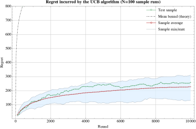
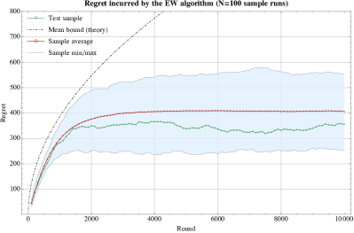
Figure 2. Performance of the UCB and EW algorithms in a channel selection problem with $A=16$ channels and random occupancy statistics. The user’s regret (measuring the throughput gap against the best channel) quickly stabilizes, giving an error probability of as little as $1\%$ relative to the best channel.

2.3.3. Full vs. partial information

From an information-theoretic point of view, a key difference between the UCB and EW algorithms is that the former does not require any further information except for the agent’s realized payoff $\hat{u}_{t}=v_{a_{t},t}$ (the payoff obtained by choosing the arm $a_{t}$) as opposed to relying also on the knowledge of the unchosen arms. Thus, since the $\operatorname{\mathcal{O}}(\sqrt{T})$ regret guarantee of the EW algorithm relies on full information, a key question remains: is it possible for the agent to attain a no-regret state in an adversarial environment with partial information?

To address this issue, the first step is to construct an estimator for the bandit’s payoff vector based on observations of the agent’s realized payoffs. This is often achieved by the so-called importance sampling technique: if the payoff vector at stage $t$ is $v_{t}$ and the agent gains $\hat{u}_{t}=v_{a_{t},t}$ after choosing arm $a_{t}$, the otherwise unobserved payoff vector can be estimated by setting

$$\hat{v}_{a,t}=\begin{cases}\hat{u}_{t}/x_{a,t}&\quad\text{if $a=a_{t}$},\\ 0&\quad\text{otherwise},\end{cases}$$ (2.18)

where $x_{a,t}=\operatorname{\mathbb{P}}(a_{t}=a)$ is the probability with which arm $a$ is drawn based on the agent’s mixed strategy $x_{t}$ at stage $t$. The key property of the resulting estimator $\hat{v}_{t}$ is that it is unbiased, i.e.,

$$\operatorname{\mathbb{E}}[\hat{v}_{t}]=v_{t}.$$ (2.19)

As such, even if the optimizer can only observe their realized payoffs, it is possible to run the EW algorithm with $\hat{v}_{t}$ in place of $v_{t}$ (for a pseudocode implementation, see Algorithm 3).

Algorithm 3 exponential weights (EW) with importance sampling

0:  the following lines in Algorithm 2

5:  receive $\hat{u}_{t}=v_{t,a_{t}}$ and set $\hat{v}_{a}\leftarrow\hat{u}_{t}\cdot\operatorname{\mathds{1}}(a=a_{t})/x_{a}$ for all $a\in\mathcal{A}$ # payoff vector estimate

6:  set $y\leftarrow y+\gamma\hat{v}$ # score update

Doing so, a finer regret analysis reveals that the EW algorithm with partial information enjoys the regret bound [45]

$$\bar{R}_{T}\leq\frac{\log A}{\gamma}+\gamma AT.$$ (2.20)

Comparing this guarantee to the full information bound (2.15), we see that the price of learning with partial information is an effective rescaling of the horizon $T$ to $AT$. In a certain sense, this is to be expected as the agent now has to play $\operatorname{\mathcal{O}}(A)$ more times in order to get a better handle on the bandit’s payoff vector. More concretely, if the parameter $\gamma$ is optimized in terms of $A$ and $T$, we have [45]:

Theorem 2.3 (EW algorithm with partial information).

The EW algorithm with partial information and learning rate $\gamma=\sqrt{\log A/(AT)}$ enjoys the regret bound

$$\bar{R}_{T}\leq 2\sqrt{AT\log A}=\operatorname{\mathcal{O}}\left(\sqrt{AT\log A}\right).$$ (2.21)

The above bound shows that the passage from full to partial information in an adversarial environment worsens the incurred regret of the EW algorithm by a factor of $\sqrt{A}$. This gap can be tightened, but only slightly so: an information-theoretic analysis of the adversarial bandit problem [7] reveals that the mean regret of any causal algorithm with partial information is bounded from below as

$$\bar{R}_{T}=\Omega\left(\sqrt{AT}\right).$$ (2.22)

Thus, comparing Eqs. 2.17 and 2.22, we see that it is not possible to bridge the gap between full and partial information when playing against an adversary.

In recent work, Audibert and Bubeck [5] shaved off the logarithmic gap between the upper and lower bounds (2.21) and (2.22) by tweaking the exponential map in (2.13) and employing a so-called implicitly normalized forecaster (INF). As in the stochastic case, further refinements are possible depending on what assumptions are made for the adversary – see e.g., [15] for some variants. However, except for such refinements, the EW algorithm essentially provides a complete solution to adversarial bandit problems; the various bounds are summarized in Table 1.

	Minimax Regret	Achieved by
Stochastic Bandit	$\Omega(\log T)$	UCB
Adversarial (Full Info)	$\Omega(\sqrt{T})$	EW
Adversarial (Partial Info)	$\Omega(\sqrt{AT})$	EW $+$ importance sampling

Table 1. Lowest achievable (minimax) regret bounds in multi-armed bandits and algorithms that attain them (up to logarithmic factors in $A$).

3. Online Optimization

Albeit powerful, the multi-armed bandit framework relies on the important assumption that the agent’s actions are drawn from a finite set, an assumption which is not realistic in many cases of practical interest in signal processing. This calls for a new way of optimizing the agent’s choices over time; this is offered by the framework of online optimization, which we motivate and discuss below.

3.1. Elements of Convex Analysis

Much of the discussion to follow will be focused on problems with a convex structure. We thus begin by recalling some basic elements of convex analysis – for a comprehensive primer, cf. [12]; see also the recent tutorials [30] and [43] for a signal processing viewpoint.

First, a subset $\mathcal{X}$ of a $d$-dimensional real space $\mathbb{R}^{d}$ is called convex if, for all $x,x^{\prime}\in\mathcal{X}$, the line segment $[x,x^{\prime}]\equiv\{(1-\theta)x+\theta x^{\prime}:0\leq\theta\leq 1\}$ also lies in $\mathcal{X}$. If $\mathcal{X}$ is convex, a function $f\colon\mathcal{X}\to\mathbb{R}$ is called convex if

$$f((1-\theta)x+\theta x^{\prime})\leq(1-\theta)f(x)+\theta f(x^{\prime})\quad\text{for all $x,x^{\prime}\in\mathcal{X}$ and all $\theta\in[0,1]$},$$ (3.1)

i.e., when the line segment between any two points on the graph of $f$ lies above the graph itself. When (3.1) holds as a strict inequality for all $x^{\prime}\neq x$, the function $f$ is called strictly convex. As a refinement of strict convexity, $f$ is called strongly convex when the gap in the inequality (3.1) is bounded by a quadratic function, i.e., there exists some $\beta>0$ such that

$$f((1-\theta)x+\theta x^{\prime})\leq(1-\theta)f(x)+\theta f(x^{\prime})-\frac{\beta}{2}\theta(1-\theta)\lVert x^{\prime}-x\rVert^{2},$$ (3.2)

or, equivalently, if the function $f(x)-\tfrac{1}{2}\beta\lVert x\rVert^{2}$ is convex. If $f$ is sufficiently differentiable, this curvature requirement is captured by asking that the Hessian of $f$ be bounded from below as $\operatorname{Hess}(f)\succcurlyeq\beta\,\mathbf{I}$.

Taking $\mathcal{X}=\mathbb{R}^{d}$, examples of convex functions include i) affine functions of the form $f(x)=a^{\top}x+b$ for $a,b\in\mathbb{R}^{d}$; ii) quadratics of the form $f(x)=x^{\top}\mathbf{M}x$ for some positive-definite $\mathbf{M}\in\mathbb{R}^{d\times d}$; iii) the log-sum-exp function $f(x)=\log\sum_{j=1}^{d}\exp(x_{j})$ which is widely used in dictionary learning and image processing; etc. Of these examples, affine functions are convex but not strictly convex, quadratics are strongly convex when $\mathbf{M}\succ 0$, and the log-sum-exp function is strictly convex but not strongly convex.

3.2. Online Optimization

With these preliminaries at hand, we are ready to describe our core online optimization framework: At each stage $t=1,2,\dotsc$, the optimizing agent selects an action $x_{t}$ from some compact convex set $\mathcal{X}\subseteq\mathbb{R}^{d}$ and incurs a loss of $\ell_{t}(x_{t})$ based on some (a priori unknown) loss function $\ell_{t}\colon\mathcal{X}\to\mathbb{R}$ (as in the bandit case, this loss function could be determined stochastically, adversarially, or otherwise). Subsequently, the agent selects a new action $x_{t+1}$ for the next stage and the process repeats as shown below:

Process 4 Generic online decision process

0:  action set $\mathcal{X}$, sequence of loss functions $\ell_{t}\colon\mathcal{X}\to\mathbb{R}$

1:  for $t=1$ to $T$ do

2:     choose $x_{t}\in\mathcal{X}$ # action selection

3:     incur $\ell_{t}(x_{t})$ # incur loss

4:     play $x_{t}\leftarrow x_{t+1}$ # update action

5:  end for

In the above description of online decision processes, no assumptions are made about the structure of the loss functions $\ell_{t}$. Typically, depending on their properties, an appropriate adjective is affixed to the term “online optimization”; in particular, we have the following fundamental classes of online optimization problems:

• Online convex optimization: $\ell_{t}\colon\mathcal{X}\to\mathbb{R}$ is convex for all $t$.

• Online strongly convex optimization: $\ell_{t}\colon\mathcal{X}\to\mathbb{R}$ is strongly convex for all $t$.

• Online linear optimization: $\ell_{t}$ is of the form $\ell_{t}(x)=-v_{t}^{\top}x$ for some vector $v_{t}\in\mathbb{R}^{d}$ and all $t$.

Both linear and strongly convex problems form subclasses of the convex class, but they are obviously pairwise disjoint. Other classes of problems have also been studied in the literature [15], but the above are the most common ones by far. For illustration purposes, we discuss some important examples below.

3.3. Examples of Online Optimization Problems

3.3.1. Multi-armed bandits revisited

Going back to the discussion of the previous section, let $\mathcal{X}=\Delta(\mathcal{A})=\{x\in\mathbb{R}_{+}^{\mathcal{A}}:\sum_{a\in\mathcal{A}}x_{a}=1\}$ denote the simplex of probability distributions over the set of arms of a multi-armed bandit. If the agent uses mixed strategy $x_{t}\in\mathcal{X}$ at stage $t$ and the bandit’s reward vector is $v_{t}$, the agent’s mean reward will be $v_{t}^{\top}x_{t}$. Hence, in a loss-based formulation, the agent will be incurring a mean loss of

$$\ell_{t}(x_{t})=-v_{t}^{\top}x_{t}.$$ (3.3)

Thus, going back to (2.12) the agent’s (mean) regret can be reformulated as

$$\bar{R}_{T}=\max_{a\in\mathcal{A}}\sum_{t=1}^{T}\operatorname{\mathbb{E}}\left[u_{t}(a)-u_{t}(a_{t})\right]=\max_{x\in\Delta(\mathcal{A})}\sum_{t=1}^{T}v_{t}^{\top}(x-x_{t})=\max_{x\in\mathcal{X}}\sum_{t=1}^{T}[\ell_{t}(x_{t})-\ell_{t}(x)].$$ (3.4)

This gives us an alternative way of interpreting the incurred regret in a multi-armed bandit problem: it is simply the difference between the aggregate loss incurred by the agent’s chosen policy and that of the best mixed strategy in hindsight. Since losses are linear, maximizing over the entire simplex (mixed strategies) or its vertices (pure strategies) does not change anything, so the two definitions coincide. As such, all applications of MAB problems discussed in Sec. 2 fall under the umbrella of online optimization.

3.3.2. Multi-antenna communications

The next example concerns the problem of signal covariance optimization in multiple-input and multiple-output (MIMO) wireless networks [43, 34, 33]. To state it, consider the dynamic multi-user MIMO wireless network of Fig. 3 where a set of autonomous wireless devices equipped with multiple antennas seek to maximize their individual data rates. Focusing on a single transmitter for convenience, its Shannon achievable rate is given by

$$C(\mathbf{Q};\tilde{\mathbf{H}})=\log\det(\mathbf{I}+\tilde{\mathbf{H}}\mathbf{Q}\tilde{\mathbf{H}}^{{\dagger}}),$$ (3.5)

where $\mathbf{Q}$ denotes the signal covariance matrix of the focal transmitter and $\tilde{\mathbf{H}}$ its effective gain matrix [34]. By standard considerations, $C$ is concave in $\mathbf{Q}$, so its maximization is relatively easy if $\tilde{\mathbf{H}}$ is known in advance. However, since $\tilde{\mathbf{H}}$ encompasses the effects of the wireless medium (noise, pathloss, device mobility) and depends on the transmit characteristics of all interfering users (which may go on- and off-line in an ad-hoc manner), it cannot be known in advance in a time-varying environment. Thus, letting $P_{\!\max}$ denote the user’s maximum transmit power and writing $\mathcal{X}=\{\mathbf{Q}\succcurlyeq 0:\operatorname{tr}\mathbf{Q}\leq P_{\!\max}\}$ for the set of possible covariance matrices, rate maximization in a dynamic MIMO network can be formulated as an online convex optimization problem where the user seeks to minimize the incurred loss $\ell_{t}(\mathbf{Q}_{t})=-C(\mathbf{Q}_{t};\tilde{\mathbf{H}}_{t})$ against any possible sequence of dynamically determined $\tilde{\mathbf{H}}_{t}$. Energy efficiency maximization [32] and cognitive medium access [41, 31] are other important applications in MIMO systems that can be formulated as online optimization problems.

Figure 3. A MU-MIMO wireless network: solid blue arrows indicate the intended receiver, dashed red arrows indicate interference crosstalk.

3.3.3. Multimedia indexing

The last example comes from supervised metric learning for image similarity search and classification [37, 9]. The aim here is to learn a positive-definite matrix $\mathbf{X}$ shaping the Mahalanobis distance $d_{X}(\mathbf{p},\mathbf{q})$ that best captures the similarity of two images $\mathbf{p}$ and $\mathbf{q}$, based upon existing annotations or examples (supervised learning); concretely, we have:

$$d_{X}(\mathbf{p},\mathbf{q})=(\mathbf{p}-\mathbf{q})^{\top}\mathbf{X}(\mathbf{p}-\mathbf{q}).$$ (3.6)

An example is a triplet $(\mathbf{p},\mathbf{q},y)$ where $\mathbf{p}$, $\mathbf{q}$ are two images and $y$ represents their similarity score (so $y=+1$ if the images are similar and $y=-1$ otherwise). Intuitively, the Malahanobis distance performs a linear transformation of the data and computes the distance $d_{X}(\mathbf{p},\mathbf{q})=\lVert\mathbf{X}^{1/2}\mathbf{p}-\mathbf{X}^{1/2}\mathbf{q}\rVert^{2}$ in the transformed space. Then, the objective is to learn the best transformation that brings closer the similar images and separates the dissimilar ones.

Following [26], this can be formalized by asking that

• For any example $(\mathbf{p},\mathbf{q},+1)$ of similar images $\mathbf{p}$ and $\mathbf{q}$, the distance separating them should be relatively small, i.e., $d_{X}(\mathbf{p},\mathbf{q})\leq\varepsilon-1$.

• For any example $(\mathbf{p},\mathbf{q},-1)$ of dissimilar images images $\mathbf{p}$ and $\mathbf{q}$, the distance separating them should be relatively large, i.e., $d_{X}(\mathbf{p},\mathbf{q})\geq\varepsilon+1$.

In the above, $\varepsilon\geq 1$ is a threshold margin which has to be learned jointly with $\mathbf{X}$. The above requirements amount to satisfying the compact similarity constraint

$$y(\varepsilon-d_{X}(\mathbf{p},\mathbf{q}))\geq 1,$$ (3.7)

which should be met for all examples $(\mathbf{p},\mathbf{q},y)$.

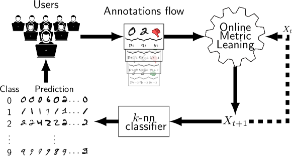
Figure 4. Online metric learning for MNIST database digit classification using the $k$-nearest neighbors classifier.

In online metric learning, the process is based on annotations that are not all available at once but become available on-the-fly (as opposed to batch methods that use offline datasets for training) [26, 25, 46]. This is particularly relevant in Internet applications where the annotations are collected continuously and in a distributed manner: there, the feedback coming from the users by scoring pairs of images (and effectively providing new examples) is exploited to improve and adapt incrementally the existent metric, as depicted in Fig. 4. Specifically, at each stage $t$, the process receives a new user annotation $(\mathbf{p}_{t},\mathbf{q}_{t},y_{t})$ and incurs the hinge loss

$$\ell_{t}(\mathbf{X}_{t},\varepsilon_{t})=\max\left\{0,1-y_{t}\left(\varepsilon_{t}-d_{X}(\mathbf{p}_{t},\mathbf{q}_{t})\right)\right\},$$ (3.8)

which penalizes the existing measure $\mathbf{X}_{t}$ and threshold $\varepsilon_{t}$ whenever the similarity constraint in (3.7) is violated. The problem’s feasible set is therefore $\mathcal{X}=\{(\varepsilon,\mathbf{X}):\varepsilon\geq 1,\mathbf{X}\succcurlyeq 0,\operatorname{tr}\mathbf{X}\leq c\}$, where the trace constraint plays the role of a relaxed rank (or sparsity) constraint enabling the reduction of computational costs, model complexity, and over-fitting effects. Fig. 4 depicts a digit classification pipeline investigated in [26] for the MNIST database (taken from http://yann.lecun.com/exdb/mnist/) exploiting the online learned metric in the $k$-nearest neighbors classifier.

3.4. Regret in Online Optimization

Recalling the discussion of the previous section, the agent’s regret in an online optimization problem is defined as

$$R_{T}=\max_{x\in\mathcal{X}}\sum_{t=1}^{T}[\ell_{t}(x_{t})-\ell_{t}(x)]=\sum_{t=1}^{T}\ell_{t}(x_{t})-\min_{x\in\mathcal{X}}\sum_{t=1}^{T}\ell_{t}(x),$$ (3.9)

i.e., as the difference between the aggregate loss incurred by the agent after $T$ stages and that of the best action in hindsight. As in the bandit case, the agent’s regret contrasts the performance of the agent’s policy $x_{t}$ to that of the optimum action

$$x^{\ast}\in\operatorname*{arg\,min}_{x\in\mathcal{X}}\sum_{t=1}^{T}\ell_{t}(x)$$ (3.10)

which minimizes the total incurred loss over the given horizon of play.

Of course, this optimum action cannot be calculated if the loss functions encountered by the optimizer are not known in advance. Consequently, the figure of merit in an online optimization problem is to design a strictly causal, online policy that achieves no regret, i.e.,

$$R_{T}=o(T),$$ (3.11)

As in the multi-armed bandit case, online optimization focuses on designing algorithms that attain the best possible regret minimization rate in (3.11), not only in terms of the horizon of play $T$, but also in terms of the multiplicative constants that come into (3.11), and which depend on the geometry and dimensionality of the optimizer’s feasible set $\mathcal{X}$. We address this issue in detail in Section 4; for now, we close this section with two important remarks relating online optimization to other optimization paradigms:

Links with static optimization

A static optimization problem in normal form can be stated as

minimize $$\quad f(x)$$ (Opt)

subject to $$\quad x\in\mathcal{X}.$$

Viewed as an online optimization problem, this would correspond to facing the same loss function $\ell_{t}=f$ at each stage. In this case, if $x_{t}$ is a no-regret policy and $f$ is convex, an immediate application of Jensen’s inequality shows that the so-called “ergodic average”

$$\bar{x}_{T}=\frac{1}{T}\sum_{t=1}^{T}x_{t}$$ (3.12)

enjoys the guarantee

$$f(\bar{x}_{T})-\min f\leq\frac{1}{T}\sum_{t=1}^{T}[f(x_{t})-\min f]\leq\frac{R_{T}}{T}.$$ (3.13)

We thus see that $\bar{x}_{T}$ converges to the solution set of (Opt) as $T\to\infty$; moreover, the rate of this convergence is controlled by the regret minimization rate of $x_{t}$. This key property of no-regret policies has been the cornerstone of a vast literature on fast optimization algorithms; for a recent overview, see [39]. As an application, in Section 4.2 (see also Fig. 7), online policies are compared to classical iterative water-filling algorithms in static MIMO networks composed of rate-driven multiple interfering users [42, 34]. This example highlights the interest of online optimization tools, especially for their theoretical guarantees and convergence properties. Indeed, providing convergence guarantees for water-filling algorithms may be very challenging. For instance, the sufficient conditions in [42] roughly require all interfering links to be dominated by the direct links, which can be rather restrictive and not necessary; in the particular case of multiple access networks (composed of multiple transmitters and one common receiver as opposed to multiple transmit-receive pairs), such conditions can never be met as the interfering links of one transmitter are the direct links of the others.

Links with stochastic optimization

The normal form of a stochastic optimization problem is

minimize $$\quad\operatorname{\mathbb{E}}[F(x;\omega)]$$ (Opt-S)

subject to $$\quad x\in\mathcal{X}$$

where $F(x;\omega)$ is a stochastic objective function that depends on a random variable $\omega$. The expectation in (Opt-S) is usually very difficult to compute (when at all possible) so, when designing algorithms to solve (Opt-S), it is assumed that $F$ is sampled at an i.i.d. realization $\omega_{t}$ of $\omega$ at each iteration. For instance, in offline metric learning for multimedia indexing, all examples are readily available in a training dataset, but they cannot be exploited simultaneously because of their prohibitive number and size [9]. To counter this, much smaller random population samples are drawn and exploited iteratively, despite the fact that the stochastic average of this sampling procedure cannot be computed.

From an online viewpoint, this corresponds to a sequence of loss functions of the form $\ell_{t}(x)=F(x;\omega_{t})$. As we discuss in detail in the next section, when each $\ell_{t}$ is convex, no regret is typically achieved by first bounding the difference $\ell_{t}(x_{t})-\ell_{t}(x)$ from above as $\nabla\ell_{t}(x_{t})^{\top}(x_{t}-x)$, and then establishing an upper bound of the form

$$\sum_{t=1}^{T}\nabla\ell_{t}(x_{t})^{\top}(x_{t}-x)\leq V_{T}$$ (3.14)

for some sublinear function $V_{T}=o(T)$. In the stochastic case where $\ell_{t}(x)=F(x;\omega_{t})$, this translates immediately to the value convergence guarantee

$$\operatorname{\mathbb{E}}[F(\bar{x}_{T};\omega)]-\min\operatorname{\mathbb{E}}[F]\leq\frac{1}{T}\sum_{t=1}^{T}\operatorname{\mathbb{E}}[\nabla\ell_{t}(x_{t})^{\top}(x_{t}-x)]\leq\frac{\operatorname{\mathbb{E}}[V_{T}]}{T}.$$ (3.15)

Thus, again, under a no-regret policy, the sequence $\bar{x}_{T}$ converges to the solution set of (Opt-S) and the rate of convergence is controlled by $V_{T}$, the mean regret minimization rate of $x_{t}$.

4. Online Algorithms and Guarantees

We now turn to the fundamental underlying question arising from the definition of the regret: How can the optimizer attain a no-regret state, and what is the associated regret minimization rate?

Of course, the answer to this question depends on the precise context of the problem at hand: the geometry and dimensionality of the agent’s action space, the structure of the problem’s objective (convex, strongly convex, etc.), the information available to the optimizer (perfect gradient observations or otherwise), are all factors that play a major role. In the following, we focus on obtaining simple answers and identifying the resulting bottlenecks; the various finer issues that arise (such as the impact of noise and feedback scarcity, etc.) are explored in Section 5.

4.1. Online Gradient Descent

The most straightforward approach for solving classic, offline optimization problems is based on (projected) gradient descent: at each stage, the algorithm takes a step against the gradient of the objective and, if necessary, projects back to the problem’s feasible region. Dating back to the seminal work of Zinkevich [50], online gradient descent (OGD) is the direct adaptation of this idea to an online context. In particular, writing

$$v_{t}=-\nabla\ell_{t}(x_{t})$$ (4.1)

for the negative gradient of the $t$-th loss function sampled at the agent’s chosen action (again at round $t$), online gradient descent (OGD) can be described via the recursion

$$x_{t+1}=\operatorname{\Pi}(x_{t}+\gamma v_{t}),$$ (4.2)

where $\operatorname{\Pi}\colon\mathbb{R}^{d}\to\mathcal{X}$ denotes the (Euclidean) projector

$$\operatorname{\Pi}(y)=\operatorname*{arg\,min}_{x\in\mathcal{X}}\ \lVert y-x\rVert^{2},$$ (4.3)

and $\gamma>0$ is a step-size parameter whose role is discussed below. (For a schematic illustration and a pseudocode implementation, see Fig. 5 and Algorithm 5 respectively.)

Algorithm 5 online gradient descent (OGD)

0:  step-size $\gamma>0$

1:  choose $x\in\mathcal{X}$ # initialization

2:  for $t=1$ to $T$ do

3:     incur loss $\hat{\ell}\leftarrow\ell_{t}(x)$ # losses revealed

4:     observe $v\leftarrow-\nabla\ell_{t}(x)$ # gradient feedback

5:     play $x\leftarrow\operatorname{\Pi}(x+\gamma v)$ # gradient step

6:  end for

Figure 5. Schematic representation of OGD (Algorithm 5).

4.1.1. Basic regret guarantees

The regret analysis of OGD is remarkably simple and intuitive, so it is worth presenting in some detail. Indeed, for any test point $p\in\mathcal{X}$, we have

$$\lVert x_{t+1}-p\rVert^{2}=\lVert\operatorname{\Pi}(x_{t}+\gamma v_{t})-p\rVert^{2}\leq\lVert x_{t}+\gamma v_{t}-p\rVert^{2}=\lVert x_{t}-p\rVert^{2}+2\gamma v_{t}^{\top}(x_{t}-p)+\gamma^{2}\lVert v_{t}\rVert^{2}.$$ (4.4)

Hence, after summing and rearranging, we obtain the “linearized” regret bound

$$\sum_{t=1}^{T}\nabla\ell_{t}(x_{t})^{\top}(x_{t}-p)=-\sum_{t=1}^{T}v_{t}^{\top}(x_{t}-p)\leq\frac{1}{2\gamma}\lVert x_{1}-p\rVert^{2}+\frac{\gamma}{2}\sum_{t=1}^{T}\lVert v_{t}\rVert^{2}.$$ (4.5)

With $\ell_{t}$ convex, the first-order condition $\ell_{t}(x_{t})-\ell_{t}(p)\leq\nabla\ell_{t}(x_{t})^{\top}(x_{t}-p)$ yields

$$R_{T}\equiv\max_{p\in\mathcal{X}}\sum_{t=1}^{T}[\ell_{t}(x_{t})-\ell_{t}(p)]\leq\frac{\operatorname{diam}(\mathcal{X})^{2}}{2\gamma}+\frac{\gamma}{2}\sum_{t=1}^{T}\lVert v_{t}\rVert^{2},$$ (4.6)

where $\operatorname{diam}(\mathcal{X})\equiv\max_{x,x^{\prime}\in\mathcal{X}}\lVert x^{\prime}-x\rVert$ denotes the (Euclidean) diameter of $\mathcal{X}$. Consequently, if we further assume that each $\ell_{t}$ is $L$-Lipschitz continuous (so $\lVert v_{t}\rVert\leq L$ for all $t$), we get

$$R_{T}\leq\frac{\operatorname{diam}(\mathcal{X})^{2}}{2\gamma}+\frac{\gamma L^{2}T}{2}.$$ (4.7)

Thus, optimizing the method’s step-size $\gamma$ as a function of the horizon $T$, we finally obtain:

Theorem 4.1 (Worst-case regret of OGD).

Against $L$-Lipschitz convex losses, the OGD algorithm with step-size $\gamma=(\operatorname{diam}(\mathcal{X})/L)/\sqrt{T}$ enjoys the regret bound

$$R_{T}\leq\operatorname{diam}(\mathcal{X})L\sqrt{T}.$$ (4.8)

As in the case of adversarial bandits, this result is quite remarkable: it shows that a) Cover’s impossibility result does not extend to problems with a convex – albeit possibly deterministic – structure; and b) the passage from discrete to continuous action spaces does not worsen the achievable regret bounds in terms of the horizon of play. In fact, Theorem 4.1 provides a key insight into what is needed to beat an adversary at its own game: convexification. The use of mixed strategies (randomization) which played a crucial role in achieving no regret against an adversarial bandit can now be seen as an instance of convexifying the problem’s structure: by looking at the mean (linear) rewards over the simplex of probability distributions (a convex set), the adversary can no longer trap the optimizer in a perpetual “ping pong” between extremes. In essence, the existence of intermediate strategies (convex combinations of pure strategies) effectively mitigates the adversary’s choices and provides the basis for achieving no regret.

4.1.2. Minimax regret and refinements

The guarantees of Theorem 4.1 cannot be improved in general: indeed, since adversarial multi-armed bandits fall under the umbrella of online linear optimization, it is not possible to achieve a worst-case guarantee better than $\Omega(\sqrt{T})$ when facing linear losses. More precisely, as was shown by Abernethy et al. [1], an informed adversary choosing linear losses of the form $\ell_{t}(x)=-{v_{t}}{x}$ with $\lVert v_{t}\rVert\leq L$ can impose regret no less than

$$R_{T}\geq\frac{\operatorname{diam}(\mathcal{X})L}{2\sqrt{2}}\sqrt{T}.$$ (4.9)

The minimax bound (4.9) above suggests there is little hope of improving on the regret minimization rate of OGD given by (4.8). Nevertheless, despite this negative result, the optimizer can achieve significantly lower regret when facing strongly convex losses. More precisely, if each $\ell_{t}$ is $\beta$-strongly convex, Hazan et al. [24] showed that a slight modification of the OGD algorithm enjoys the logarithmic regret guarantee

$$R_{T}\leq\frac{1}{2}\frac{L^{2}}{\beta}\log T=\operatorname{\mathcal{O}}(\log T).$$ (4.10)

Remarkably, in the class of strongly convex functions, this guarantee is tight, even up to the multiplicative constant in (4.10). In particular, Abernethy et al. showed in [1] that if the adversary is restricted to quadratic convex functions of the form $\ell_{t}(x)=\frac{1}{2}x^{\top}\mathbf{M}_{t}x-v_{t}^{\top}x+c$ with $\mathbf{M}_{t}\succcurlyeq\beta\,\mathbf{I}$, the optimizer’s worst-case regret cannot be better than

$$R_{T}\geq\frac{1}{2}\frac{L^{2}}{\beta}\log T.$$ (4.11)

The above shows that the rate of regret minimization in online convex optimization depends crucially on the curvature of the loss functions encountered. Against arbitrary loss functions, the optimizer cannot hope to do better than $\Omega(\sqrt{T})$ in general; however, if the optimizer’s losses possess a strictly positive global curvature, the optimizer’s worst-case guarantee drops down to $\operatorname{\mathcal{O}}(\log T)$. For convenience, we collect these guarantees in Table 2.

	Minimax Regret	Worst-Case
Convex Losses	$\Omega(LT^{1/2})$	$\operatorname{\mathcal{O}}(LT^{1/2})$
Linear Losses	$\Omega(LT^{1/2})$	$\operatorname{\mathcal{O}}(LT^{1/2})$
$\beta$-Strongly Convex	$\Omega(\beta^{-1}L^{2}\log T)$	$\operatorname{\mathcal{O}}(\beta^{-1}L^{2}\log T)$

Table 2. Regret achieved by OGD (Algorithm 5) against $L$-Lipschitz convex losses.

As an illustrative example, consider the maximization of transmit energy efficiency in multi-user MIMO networks, defined here as the ratio between throughput and power consumption. In [32], it was shown that if each user applies an online gradient policy, they are able to track their mean optimal transmit covariance matrix in a distributed manner. This is illustrated in Fig. 6 for mobile users with very different mobility characteristics, both pedestrian and vehicular. Specifically, in Fig. 6, the users’ policy is compared to several policies: a) the instantaneous optimum policy that varies over time (labeled “Optimum”); b) a uniform power allocation scheme over antennas and frequency carriers (“Uniform”); and c) the best fixed policy in hindsight (“Oracle”). Remarkably, even under rapidly changing channel conditions, the users’ online policy quickly converges to the maximum value and tracks its variations remarkably well and consistently outperforms the fixed oracle solution – a behavior consistent with the no-regret property of OGD.

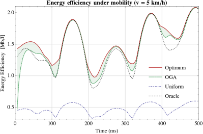
(a) Energy efficiency under low mobility

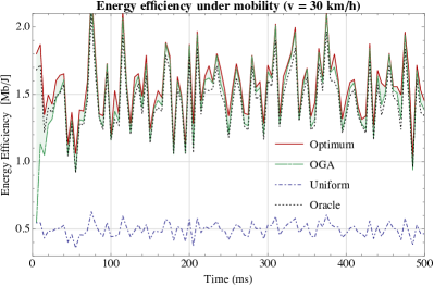
(b) Energy efficiency under high mobility

Figure 6. Performance of an online gradient policy in a dynamic setting with mobile users seeking to optimize their transmit energy efficiency [32]. The users’ achieved energy efficiency tracks its (evolving) maximum value remarkably well, even under rapidly changing channel conditions.

4.2. Online Mirror Descent

Even though the worst-case regret guarantee of OGD is essentially tight, there is an important gap hidden in the problem’s geometry. This is best explained by going back to the adversarial multi-armed bandit problem: as discussed in Section 3, MABs can be seen as an online linear problem with feasible region $\mathcal{X}=\Delta(\mathcal{A})=\{x\in\mathbb{R}^{x}:\sum_{a\in\mathcal{A}}x_{a}=1\}$ and linear loss functions of the form $\ell_{t}(x)=-v_{t}^{\top}x$ where $\lvert v_{a,t}\rvert\leq 1$ for all $a\in\mathcal{A}$ and all $t=1,2,\dotsc,T$. This implies that the Lipschitz constant of the bandit’s loss functions can be as high as

$$\textstyle L=\max\left\{\sqrt{\sum_{a\in\mathcal{A}}v_{a}^{2}}:\lvert v_{a}\rvert\leq 1\right\}=\sqrt{1^{2}+\dotsm+1^{2}}=\sqrt{A},$$ (4.12)

so the regret guarantee (4.8) of OGD becomes

$$R_{T}\leq\sqrt{AT}.$$ (4.13)

Compared to the $\operatorname{\mathcal{O}}(\sqrt{T\log A})$ worst-case regret guarantee of the EW algorithm (cf. Section 2), the above indicates a gap of the order of $\operatorname{\mathcal{O}}(\sqrt{A/\log A})$ between the two algorithms – and this, despite the fact that OGD implicitly assumes full knowledge of the gradient vector $v_{t}$ at each round. In this way, we are faced with an apparent paradox: how can the $\operatorname{\mathcal{O}}(\sqrt{T\log A})$ regret guarantee of the EW algorithm be reconciled with the $\Omega(\sqrt{AT})$ minimax bound of Eq. 4.9 for online linear problems with $\sqrt{A}$-Lipschitz losses?

The answer to this paradox lies in the different sets of the reward vectors $v_{t}$ chosen by the adversary. In online linear problems with $\sqrt{A}$-Lipschitz losses, $v_{t}$ is drawn from the Euclidean ball of radius $\sqrt{A}$ (i.e., $\lVert v_{t}\rVert\leq\sqrt{A}$). By contrast, in multi-armed bandit problems, the reward vector $v_{t}$ lies in the hypercube $[-1,1]^{A}$ (since $\lvert v_{a,t}\rvert\leq 1$). The hypercube is strictly contained in the (much) larger Euclidean ball so, heuristically, an adversarial multi-armed bandit is more constrained and cannot cause as much damage.

Geometrically, this highlights a crucial difference between the $\ell^{\infty}$ sup-norm and the ordinary (Euclidean) $\ell^{2}$ norm, which in turn explains the performance gap between the EW and OGD algorithms in online linear problems. By moving beyond the Euclidean norm and geometry might bridge this gap and lift the so-called curse of dimensionality in general online convex optimization problems. Especially in the world of Big Data, many problems of practical interest have state spaces of huge dimension, so descent methods must be finely tuned to the problem’s geometry in order to attain an optimal regret minimization rate.

Algorithm 6 online mirror descent (OMD)

0:  $K$-strongly convex regularizer $h\colon\mathcal{X}\to\mathbb{R}$, step-size $\gamma>0$

1:  choose $x\in\mathcal{X}$ # initialization

2:  for $t=1$ to $T$ do

3:     incur loss $\hat{\ell}\leftarrow\ell_{t}(x)$ # losses revealed

4:     observe $v\leftarrow-\nabla\ell_{t}(x)$ # gradient feedback

5:     play $x\leftarrow P_{x}(\gamma v)$ # mirror step

6:  end for

4.2.1. Mirror descent

A systematic way to exploit the geometry of the problem is via the method of online mirror descent (OMD) [44]. To illustrate the core components of the method (which can be traced back to the seminal work of Nemirovski and Yudin [38] for offline problems), it is convenient to rewrite the Euclidean update step (4.2) of OGD as

$$x_{t+1}=\operatorname{\Pi}(x_{t}+\gamma v_{t}) =\operatorname*{arg\,min}_{x\in\mathcal{X}}\ \tfrac{1}{2}\lVert x_{t}+\gamma v_{t}-x\rVert^{2}$$

$$=\operatorname*{arg\,min}_{x\in\mathcal{X}}\ \big{\{}\tfrac{1}{2}\lVert x_{t}-x\rVert^{2}+\tfrac{1}{2}\lVert\gamma v_{t}\rVert^{2}+\gamma v_{t}^{\top}(x_{t}-x)\big{\}}$$

$$=\operatorname*{arg\,min}_{x\in\mathcal{X}}\ \big{\{}\gamma v_{t}^{\top}(x_{t}-x)+D(x,x_{t})\big{\}},$$ (4.14)

where we have defined

$$\textstyle D(p,x)=\frac{1}{2}\lVert p-x\rVert^{2}=\frac{1}{2}\lVert p\rVert^{2}-\frac{1}{2}\lVert x\rVert^{2}-x^{\top}(p-x).$$ (4.15)

The key novelty of mirror descent is to replace this quadratic term by the so-called Bregman divergence

$$D_{h}(p,x)=h(p)-h(x)-\nabla h(x)^{\top}(p-x),$$ (4.16)

where $h\colon\mathcal{X}\to\mathbb{R}$ is a smooth $K$-strongly convex function (usually referred to as a regularizer). In so doing, we obtain the online mirror descent (OMD) algorithm

$$x_{t+1}=P_{x_{t}}(\gamma_{t}v_{t}),$$ (4.17)

where the mirror-prox operator $P$ is defined as

$$P_{x}(v)=\operatorname*{arg\,min}_{x^{\prime}\in\mathcal{X}}\ \left\{v^{\top}(x-x^{\prime})+D_{h}(x^{\prime},x)\right\},$$ (4.18)

and, as before, $v_{t}=-\nabla\ell_{t}(x_{t})$ denotes the negative gradient of the loss function of the $t$-th sampled at $x_{t}$. (For a pseudocode implementation, see Algorithm 6.)

4.2.2. Examples

Before delving into the regret guarantees of the OMD algorithm, it is worth discussing some important examples in detail:

Example 4.1 (Euclidean regularization).

As we discussed above, the regularizer $h(x)=\frac{1}{2}\lVert x\rVert^{2}$ yields the archetypal OGD algorithm (4.2). As such, all results obtained for OMD also carry over to OGD.

Example 4.2 (Entropic regularization).

Another important instance of the OMD method is when the problem’s feasible region $\mathcal{X}$ is the unit simplex of $\mathbb{R}^{d}$ and the regularizer is the (negative) Gibbs–Shannon entropy

$$h(x)=\sum_{j=1}^{d}x_{j}\log x_{j}.$$ (4.19)

A short calculation shows that the resulting mirror-prox operator is given by the exponential mapping

$$P_{x}(v)=\frac{(x_{j}\exp(v_{j}))_{j=1}^{d}}{\sum_{k=1}^{d}x_{k}\exp(v_{k})}$$ (4.20)

which in turn leads to the exponentiated gradient (EG) algorithm:

$$x_{j,t+1}=\frac{x_{j,t}\exp(\gamma v_{j,t})}{\sum_{k=1}^{d}x_{k,t}\exp(\gamma v_{k,t})}.$$ (4.21)

Importantly, going back to the EW algorithm (2.13) for multi-armed bandits, we readily get

$$x_{j,t+1}\propto\exp(y_{j,t+1})=\exp(y_{j,t}+\gamma v_{j,t})\propto x_{j,t}\exp(\gamma v_{j,t}).$$ (4.22)

Thus, by normalizing, we see that OMD with entropic regularization is simply the EW algorithm. This remarkable observation sheds further light on the structure of the EW algorithm: despite their very different origins, exponential weights and gradient descent are different sides of the same coin – mirror descent.

Algorithm 7 matrix exponential learning (MXL)

0:  step-size $\gamma>0$

1:  $\mathbf{Y}\leftarrow 0$ # initialization

2:  for $t=1$ to $T$ do

3:     set $\mathbf{X}\leftarrow\exp(\mathbf{Y})/[1+\operatorname{tr}(\exp(\mathbf{Y}))]$ # matrix exponentiation

4:     incur loss $\hat{\ell}\leftarrow\ell_{t}(\mathbf{X})$ # losses revealed

5:     observe $\mathbf{V}\leftarrow-\nabla\ell_{t}(\mathbf{X})$ # gradient feedback

6:  end for

Example 4.3 (Matrix exponential learning).

Our last example concerns learning with matrices and is of particular relevance to MIMO communications [43, 41, 34, 33]. When optimizing signal covariance matrices in such systems, the problem’s feasible region is often a spectrahedron of the form

$$\boldsymbol{\mathcal{X}}=\{\mathbf{X}\in\mathbb{R}^{d\times d}:\mathbf{X}\succcurlyeq 0,\,\operatorname{tr}{\mathbf{X}}\leq 1\}.$$ (4.23)

A tailor-made regularizer for this type of constraints is given by the (negative) von Neumann entropy

$$h(\mathbf{X})=\operatorname{tr}[\mathbf{X}\log\mathbf{X}]+(1-\operatorname{tr}\mathbf{X})\log(1-\operatorname{tr}\mathbf{X}).$$ (4.24)

As was shown in [34, 33], this choice of regularizer yields the matrix exponential learning (MXL) algorithm

$$\mathbf{Y}_{t+1} =\mathbf{Y}_{t}+\gamma\mathbf{V}_{t}$$ (4.25)

$$\mathbf{X}_{t+1} =\frac{\exp(\mathbf{Y}_{t+1})}{1+\operatorname{tr}[\exp(\mathbf{Y}_{t+1})]}$$

where $\mathbf{V}_{t}=-\nabla_{\mathbf{X}_{t}}\ell_{t}(\mathbf{X}_{t})$ is the matrix gradient of the $t$-th round loss function (for a pseudocode implementation, see Algorithm 7). A very appealing property of the exponential update in (4.25) is that it ensures positive-definiteness in an elegant and lightweight manner compared to the Euclidean projection on the positive-definite cone (which requires solving a convex optimization problem at each stage). Moreover, this algorithm exhibits very fast convergence rates for throughput and energy efficiency maximization in wireless networks, greatly outperforming traditional algorithms based on water-filling [34, 33]; for an illustration of the algorithm’s performance in MIMO systems, see Fig. 7.

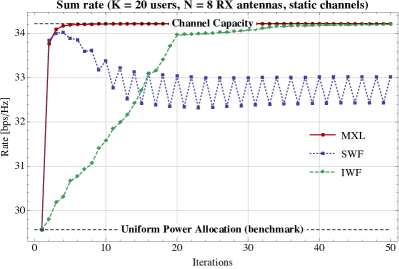
(a) Sum rate for 20 users and 8 receive antennas

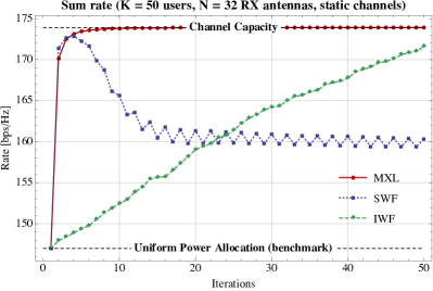
(b) Sum rate for 50 users and 32 receive antennas

Figure 7. Performance comparison between the MXL algorithm with water-filling methods in a static uplink setting with one base station and multiple transmitters driven by their own rates [34]. IWF converges slowly because only one user updates its input covariance per iteration; SWF is faster but does not always converge due to cycles in the update process. On the contrary, the MXL algorithm converges within a few iterations even for large numbers of users.

To highlight the range of the MXL algorithm, we also consider below its application to the multimedia indexing problem described in Section 3. Specifically, in Fig. 8, we compare the Euclidean metric with the online metric that was learned by the MXL algorithm, and a different online metric based on the mirror descent for metric learning (MDML) algorithm of [26]. In more detail, we tested the MDML variant based on the Frobenius norm regularization (as opposed to the entropic regularization). Fig. 8 illustrates that MXL performs best in terms of classification test errors on three well-known datasets: Iris, Wine and MNIST. both the mean and variance of the results with respect to the random dataset splitting between train and test over $200$ runs are plotted (except for the MNIST data in which the pre-defined sets were used). For a detailed description of the experimental setup used to obtain these plots (dataset description, choice of the train and test datasets, step-sizes, etc.) we refer the reader to the online report [10].

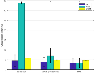
(a) Classification errors on Iris, Wine and MNIST.

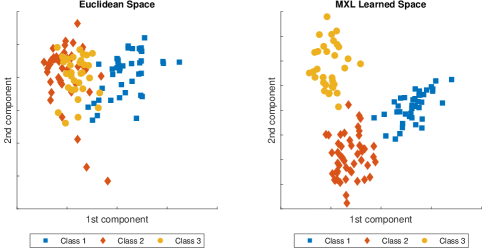
(b) Principal data components in the Euclidean and the transformed space via MXL on the Wine dataset.

Figure 8. Performance comparison between a Euclidean metric, and two online metrics based on mirror descent: the MDML in [26] and MXL, on three different datasets (Iris, Wild and MNIST). Both online metrics always outperform the Euclidean metric and the MXL algorithm provides the best online learned metric. In the Wine dataset, in which the Euclidean representation is quite ill-suited for classification, the MXL algorithm provides the best linear transformation, which successfully separates the images into the three classes.

4.2.3. Regret guarantees

The basic worst-case guarantee of OMD is as follows [45, 13, 27]:

Theorem 4.2 (Worst-case regret of OMD).

Against $L$-Lipschitz convex losses, the OMD algorithm based on a $K$-strongly convex regularizer $h$ enjoys the regret bound

$$R_{T}\leq 2L\sqrt{\frac{\max h-\min h}{2K}T},$$ (4.26)

achieved by taking the step-size $\gamma=L^{-1}\sqrt{2K(\max h-\min h)/T}$.

An important remark in the above is that the strong convexity and Lipschitz constants $K$ and $L$ need not be taken with respect to the Euclidean norm. When they are, Theorem 4.2 readily yields the $\operatorname{\mathcal{O}}(L\sqrt{T})$ regret guarantee of OGD. For the EW algorithm, the entropic regularizer (4.19) is $1$-strongly convex with respect to the taxicab ($\ell^{1}$) norm [45] and $\max h-\min h=\sum_{j=1}^{d}\frac{1}{d}\log d=\log d$, leading to the $\operatorname{\mathcal{O}}(\sqrt{T\log A})$ bound (2.15) (since $A\equiv d$). Finally, for the MXL algorithm, the von Neumann regularizer $h$ is $1$-strongly convex relative to the nuclear matrix norm ($\lVert\mathbf{X}\rVert_{1}=\operatorname{tr}\lvert\mathbf{X}\rvert$) and $\max h-\min h=\log d$, leading to the regret bound

$$R_{T}\leq L\sqrt{2T\log d}.$$ (4.27)

Remarkably, the regret bound of the EW and MXL algorithms coincide, even though the latter is run in a space of much greater dimension ($d\times d$ versus $d$ respectively).

We summarize these results in Table 3. The main take-away from this table is that OMD enjoys the same $\sqrt{T}$ rate as OGD, but the multiplicative constants are optimized relative to the dimension and geometry of the problem. This logarithmic reduction is of immense value to real-world Big Data problems that suffer from the curse of dimensionality. As a result, the systematic design of tailor-made OMD algorithms for arbitrary problem geometries has attracted considerable interest in the literature and remains a vigorously researched question, often resembling a form of art.

	Region	Losses	Regret
OGD	Unit ball	$\lVert v_{t}\rVert\leq 1$	$\operatorname{\mathcal{O}}(\sqrt{T})$
EW	Simplex	$\lVert v_{t}\rVert_{\infty}\leq 1$	$\operatorname{\mathcal{O}}(\sqrt{T\log d})$
MXL	Spectrahedron	$\lvert\operatorname{eig}(\mathbf{V}_{t})\rvert\leq 1$	$\operatorname{\mathcal{O}}(\sqrt{T\log d})$

Table 3. Regret achieved by OMD strategies in various geometries.

5. Additional Considerations

In this final section, we discuss some further aspects of regret minimization that are of particular relevance to signal processing and its applications.

5.1. Imperfect feedback

We begin by discussing the quality and amount of feedback available to the optimizer. Indeed, throughout the analysis of the previous section, it was tacitly assumed that the optimizer had access to a black-box feedback mechanism – an oracle – which, when called, provided perfect gradient observations for the loss function of each stage. In the multi-armed bandit language of Section 2, this corresponds to the “full information” case, i.e., when the agent has full knowledge of the payoff vector $v_{t}$ at each stage (meaning the payoff of each arm – chosen or not). In practical situations (e.g., throughput maximization in a fast-fading wireless medium), such information might be difficult – or even impossible – to come by, so the relevance and applicability of the online algorithms we have discussed so far is put to the test.

To model imperfections in the optimizer’s feedback, we will focus on an application-agnostic framework where, at each stage $t=1,2,\dotsc$, the optimizer receives a noisy, imperfect estimate $\hat{v}_{t}$ of the true gradient $v_{t}=-\nabla\ell_{t}(x_{t})$. For this estimate, we make the standard statistical assumptions that it is unbiased and bounded in mean square, i.e.,

$$\operatorname{\mathbb{E}}[\hat{v}_{t}\nonscript\>|\nonscript\>\mathopen{}\mathcal{F}_{t-1}]=v(x_{t}),$$ (5.1a)

and

$$\operatorname{\mathbb{E}}[\lVert\hat{v}_{t}\rVert^{2}\nonscript\>|\nonscript\>\mathopen{}\mathcal{F}_{t-1}]\leq V^{2}\quad\text{for some finite $V>0$},$$ (5.1b)

where $\mathcal{F}_{t}$ denotes the history of play up to stage $t$ (inclusive). These bare-bones assumptions simply indicate that there is no systematic error in the optimizer’s gradient measurements and that the observed error cannot become unreasonably large with high probability. This is true for most statistical distributions used to describe error processes in practice – ranging from uniform and (sub-)Gaussian to log-normal, exponential, and Lévy-type models – so we will maintain this assumption throughout what follows.

Of course, given that the feedback to the optimizer is now a stochastic process, the incurred regret will also be random. On that account, the figure of merit will now be the optimizer’s mean regret

$$\bar{R}_{T}=\max_{x\in\mathcal{X}}\sum_{t=1}^{T}\operatorname{\mathbb{E}}[\ell_{t}(x_{t})-\ell_{t}(x)],$$ (5.2)

which is the direct extension of the corresponding regret measure (2.12) for multi-armed bandit problems (cf. Section 2). Then, focusing for simplicity on the OGD algorithm, we have the following worst-case guarantee [13, 27]:

Theorem 5.1 (Worst-case regret of OGD with imperfect feedback).

Against convex losses, the OGD algorithm with step-size $\gamma=\operatorname{diam}(\mathcal{X})/\sqrt{V^{2}T}$ and noisy gradient feedback satisfying (5.1) enjoys the worst-case guarantee

$$\bar{R}_{T}\leq\operatorname{diam}(\mathcal{X})V\sqrt{T}=\operatorname{\mathcal{O}}(\sqrt{T}).$$ (5.3)

Remarkably, despite all the uncertainty, the worst-case regret of OGD with noisy feedback is of the same order in $T$ as in the perfect information case (cf. Theorem 4.1 in Section 4). That being said, the noise does deteriorate the algorithm’s performance in two important ways:

1. The regret bound (5.3) depends linearly on the second moment of the optimizer’s feedback (which could become quite high if the optimizer only has access to low-quality observations with a lot of noise).

2. The optimizer must be able to estimate the variance of the noise in order to run OGD.

Especially the latter could have important ramifications for the agent’s regret: if the optimizer “plays it safe” and overestimates the variance of the noise, the incurred regret will grow commensurately because of the second moment factor $V$ in (5.3). This quantifies the impact of errors and observation noise in the performance of OGD.

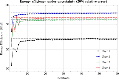
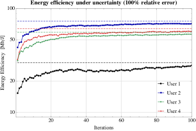
Figure 9. Energy efficiency of an online gradient policy with imperfect measurements and observation errors [32]. Even under very high uncertainty, when the gradient estimation lies within $100\%$ of its true value, the system converges within a few tens of iterations to a stable, no-regret state (dashed line).

To asses the impact of the noisy estimation in a concrete example, we plot the energy efficiency of the online gradient algorithm in [32] in Fig. 6 for four arbitrarily chosen users (see also the corresponding discussion in Section 4.1). Here, the channels are assumed to remain static to better isolate this effect. Although the system’s rate of equilibration is affected by the intensity of the noise, the system still equilibrates within a few tens of iterations, even in the presence of very high uncertainty. Other applications to rate maximization problems via OMD can be found in [31, 34].

5.2. Zeroth-order feedback

The noisy feedback case can be seen as the precursor to a much more challenging question: can the optimizer attain a no-regret state with no gradient feedback whatsoever?

This question is sometimes referred to as “bandit online optimization” (in reference to the multi-armed bandit problem) or “online optimization with zeroth-order feedback” (in contrast to first-order feedback, i.e., gradient information). The motivation for it is clear: in many practical applications (such as multi-user communication systems), gradient calculations are completely beyond the optimizer’s reach (noisy or otherwise), especially if the loss function itself is not revealed. In that case, the only feedback available to the agent is the actual incurred loss, and the agent must choose a descent direction to follow based only on this minimal piece of information.

In the multi-armed bandit problem, this is achieved by means of the importance sampling technique we described in Section 2 (cf. Algorithm 3). However, in more general online optimization problems, importance sampling cannot be applied because there is a continuum of points to sample, and also because the value of a function at a given point (a scalar) carries no information about its gradient (a vector). Thus, to gain such information, it is important to inject some “directionality” that could generate a vector out of a scalar. This is precisely the key idea behind the so-called simultaneous stochastic approximation (SSA) method of Spall [48] where the gradient is estimated by artificially sampling the function not at the point of interest, but at a nearby, randomly chosen point.

To illustrate the method, it is convenient to begin with the one-dimensional case, i.e., functions defined over the real line. Specifically, suppose that we seek to estimate the derivative of a function $f\colon\mathbb{R}\to\mathbb{R}$ at some target point $\hat{x}$ using a single evaluation thereof. By definition, this derivative can be approximated by the difference quotient

$$f^{\prime}(\hat{x})\approx\frac{f(\hat{x}+\delta)-f(\hat{x}-\delta)}{2\delta},$$ (5.4)

with the approximation becoming exact as $\delta\to 0^{+}$. Of course, this estimate requires two function evaluations (at $\hat{x}+\delta$ and $\hat{x}-\delta$), but it also suggests the following approach: simply make a (uniform) random draw from $\{\pm 1\}$ and sample $f$ at $\hat{x}\pm\delta$ accordingly. Letting $z\in\{\pm 1\}$ denote the outcome of this draw, the difference quotient above can be rewritten as

$$\frac{f(\hat{x}+\delta)-f(\hat{x}-\delta)}{2\delta}=\frac{1}{\delta}\left[\frac{1}{2}f(\hat{x}+\delta)-\frac{1}{2}f(\hat{x}-\delta)\right]=\frac{1}{\delta}\operatorname{\mathbb{E}}[f(\hat{x}+\delta z)\,z].$$ (5.5)

i.e., as the expectation of the random variable $f(\hat{x}+\delta z)z$. Thus, going back to (5.4), we see that $f^{\prime}(\hat{x})$ can be approximated to $\operatorname{\mathcal{O}}(\delta)$ by the single-shot estimator $\delta^{-1}f(\hat{x}+\delta z)\,z$.

Extending this construction to functions defined on $\mathbb{R}^{d}$ gives rise to the estimator

$$\frac{d}{\delta}f(\hat{x}+\delta z)\,z,$$ (5.6)

where $z$ is now drawn uniformly from the unit sphere $\mathbb{S}^{d}$ and the factor $d$ has been included for dimensional scaling reasons. As in the one-dimensional case, the bias of the estimator vanishes in the limit $\delta\to 0^{+}$: more precisely, for positive $\delta>0$ and $L$-Lipschitz $f$, we have

$$\operatorname{\mathbb{E}}\left[\frac{d}{\delta}f(\hat{x}+\delta z)\,z\right]=\nabla f_{\delta}(\hat{x}),$$ (5.7)

where $f_{\delta}$ is a “$\delta$-smoothed” approximation of $f$ with $\lvert f_{\delta}(\hat{x})-f(\hat{x})\rvert\leq L\delta$. In other words, the single-shot estimator (5.6) provides a reasonable approximation of $\nabla f(\hat{x})$, up to a bias of at most $\operatorname{\mathcal{O}}(\delta)$.

Algorithm 8 online gradient descent with zeroth-order feedback (OGD-0)

0:  step-size $\gamma>0$, exploration factor $\delta>0$

1:  choose pivot point $\hat{x}$ # initialization

2:  for $t=1$ to $T$ do

3:     draw $z$ uniformly from $\mathbb{S}^{d}$ # exploration direction

4:     play $x\leftarrow\hat{x}+\delta z$ # choose action

5:     incur loss $\hat{\ell}\leftarrow\ell_{t}(x)$ # losses revealed

6:     set $\hat{v}\leftarrow-\frac{d}{\delta}\hat{\ell}\cdot z$ # estimate gradient

7:     set $\hat{x}\leftarrow\operatorname{\Pi}(\hat{x}+\gamma\hat{v})$ # update pivot

8:  end for

Figure 10. Schematic representation of OGD-0 (Algorithm 8). To ensure feasibility, the projected iterate is mapped to the $\delta$-shrunk region $\mathcal{X}_{\delta}$.

The above is the cornerstone of the “gradient descent without a gradient” methodology of [17]. In particular, the main idea of this method is to apply a projected descent scheme to generate an online sequence of pivot points $\hat{x}_{t}$. These points are not played by the optimizer, but they act as base points (“pivots”) to select an action at each stage based on the perturbation model

$$x_{t}=\hat{x}_{t}+\delta z_{t},$$ (5.8)

with $z_{t}$ drawn i.i.d. from the unit sphere $\mathbb{S}^{d}$ of $\mathbb{R}^{d}$. In so doing, the agent can follow the zeroth-order technique outlined above to simultaneously estimate the (negative) gradient of $\ell_{t}$ at $\hat{x}_{t}$ as

$$\hat{v}_{t}=-\frac{d}{\delta}\ell_{t}(x_{t})\,z_{t}.$$ (5.9)

Of course, this is not an estimate of the loss gradient at $x_{t}$. However, since the distance between the pivot and the agent’s chosen action is $\operatorname{\mathcal{O}}(\delta)$, the difference is not too big: optimistically, it should be enough to generate a descent step. With this in mind, we obtain the following recursive scheme for running online gradient descent with zeroth-order feedback (OGD-0):

$$x_{t} =\hat{x}_{t}+\gamma z_{t}$$ (5.10)

$$\hat{v}_{t} =-\frac{d}{\delta}\ell_{t}(x_{t})\,z_{t}$$

$$\hat{x}_{t+1} =\operatorname{\Pi}(\hat{x}_{t}+\gamma\hat{v}_{t})$$

with $\hat{x}_{1}$ initialized arbitrarily (for a pseudocode implementation, see Algorithm 8).

Before proceeding with the analysis of OGD-0, two remarks are in order: The first concerns the bias-variance dilemma: the bias of the estimator (5.9) can be made arbitrarily small but, in so doing, the estimator’s variance explodes. In this way, it is impossible to satisfy both branches of the statistical assumption (5.1): the zeroth-order estimator (5.9) can either have small bias or small variance, but not both.

The second important consideration is that if the pivot point $\hat{x}_{t}$ lies too close to the boundary of $\mathcal{X}$, the chosen action $x_{t}=\hat{x}_{t}+\delta z_{t}$ may lie outside the problem’s feasible region. To account for this feasibility issue, one can keep the method’s pivots away from the boundary of $\mathcal{X}$ by re-projecting them onto a “$\delta$-shrunk” sub-region of $\mathcal{X}$ (for a schematic illustration, see Fig. 10). This introduces a further error of order $\operatorname{\mathcal{O}}(\delta)$ in the mix, but since all other estimation errors are of the same order, it does not affect the algorithm’s qualitative behavior. To streamline our presentation and keep our notation as light as possible, we will not carry around this adjustment in the definition of OGD-0 but we will tacitly assume that it always takes place if/when needed.

With all this at hand, it can be shown that OGD-0 enjoys the following guarantee [17, 45]:

Theorem 5.2 (Worst-case regret of OGD-0).

Against $L$-Lipschitz convex losses, the OGD-0 algorithm enjoys the worst-case guarantee

$$\bar{R}_{T}=\operatorname{\mathcal{O}}(\sqrt{dL}T^{3/4}),$$ (5.11)

achieved by taking $\gamma=(2T)^{-1/2}B/[d(\ell_{\max}/\delta+L)]$ and $\delta=T^{-1/4}\sqrt{dB\ell_{\max}/(3L)}$, with $\ell_{\max}$ denoting the agent’s maximum possible loss (i.e., $\ell_{t}\leq\ell_{\max}$ for all $t$) and $B=\max_{x\in\mathcal{X}}\lVert x\rVert$.

The complicated expressions for the operational parameters of OGD-0 illustrate the delicate dependence of the algorithm’s performance on balancing exploration versus exploitation. If the exploration parameter $\delta$ is too large, the algorithm’s gradient estimator will gain in terms of precision (variance) but lose in terms of accuracy; conversely, for small $\delta$, the estimated gradient will be relatively accurate in the mean, but with immense variability. This is a consequence of the fact that, in general, exploring a nonlinear function is much more difficult than exploring a bandit with a finite number of arms.

The above also explains the difficulty in closing the gap between the $\operatorname{\mathcal{O}}(T^{3/4})$ regret minimization rate of Theorem 5.2 and the $\operatorname{\mathcal{O}}(T^{1/2})$ rate that can be achieved when first-order feedback is available (noisy or otherwise). This gap has been closed in several cases, such as if the optimizer can sample each loss function at two points [2], if the loss functions are highly smooth [8], and other refinements of the problem. However, the case of general convex functions remains open and it is not known whether there is a fundamental gap between what is known and what is attainable with zeroth-order feedback (though it is widely believed that $\operatorname{\mathcal{O}}(\sqrt{T})$ regret should still be attainable in this case).

Remark.

Before ending the limited feedback discussion, we note that similar results to Theorems 5.1 and 5.2 also hold for general OMD algorithms. The worse-case regret with noisy feedback is of the same order as in the perfect information case, while zeroth-order feedback incurs the same drop in the rate of regret minimization.

5.3. Fixed horizon vs. anytime bounds

A further consideration regarding the information available to the optimizer is the knowledge – or not – of the horizon of play. Indeed, all the worst-case guarantees that we have discussed so far presume that $T$ is known in advance, so the various parameters of an online optimization algorithm can be fine-tuned as a function thereof. Depending on the application at hand, this assumption could be severely limiting: for instance, in the context of telecommunication networks, it is often far-fetched to assume that a wireless user can know in advance the duration of their call.

Guarantees established for problems where the duration of play is unknown are usually referred to as anytime bounds and one of the main techniques to achieve them is via the so-called doubling trick [15]. The basic idea behind this device is as follows: the optimizer chooses a fixed window consisting of $W$ rounds and plays with a no-regret algorithm optimized for $W$ stages. When this window draws to a close, the agent doubles the window length ($W\leftarrow 2W$) and restarts the algorithm, now optimized for $2W$ stages. This process then repeats as needed, until play ends – specifically, after no more than $\lceil\log_{2}(T/W)\rceil$ period doublings.

In so doing, if the chosen algorithm enjoys an upper bound of $MW^{1/2}$ when run over a fixed window of size $W$, the induced anytime bound will be

$$\smashoperator[]{\sum_{k=0}^{\lceil\log_{2}(T/W)\rceil}}M\sqrt{2^{k}W}=M\sqrt{W}\frac{\sqrt{2}^{\lceil\log_{2}(T/W)\rceil+1}-1}{\sqrt{2}-1}\leq M\sqrt{W}\,\frac{2\sqrt{T/W}}{\sqrt{2}-1}=\frac{2}{\sqrt{2}-1}M\sqrt{T}.$$ (5.12)

In other words, thanks to the doubling trick, the optimizer can achieve an anytime regret guarantee which is at most a factor of $2/(\sqrt{2}-1)$ worse than the algorithm’s fixed horizon guarantee. Moreover, this constant factor does not depend on the size of the window, so the optimizer has significant flexibility in applying the doubling trick.

Similar tricks can also be applied to the case where an algorithm guarantees a regret of $MW^{\alpha}$ for some $\alpha\in(0,1)$. In this case, it is again possible to achieve $\operatorname{\mathcal{O}}(MW^{\alpha})$ regret up to a universal multiplicative factor that depends only on $\alpha$. We leave the details as an exercise for the reader.

5.4. Dynamic regret

To conclude this section, we briefly return to the definition of the regret as the performance gap between the optimizer’s chosen policy and the best fixed action in hindsight. This definition is somewhat restrictive as it only compares the chosen policy to constant policies; ideally, the optimizer would seek to minimize the incurred dynamic regret, defined here as

$$R^{\ast}_{T}=\sum_{t=1}^{T}\left[\ell_{t}(x_{t})-\min_{x\in\mathcal{X}}\ell_{t}(x)\right].$$ (5.13)

Obviously, since $R^{\ast}_{T}$ targets the smallest possible aggregate loss $\sum_{t=1}^{T}\min_{x\in\mathcal{X}}\ell_{t}(x)$, we have $R_{T}\leq R^{\ast}_{T}$, i.e., the ordinary (static) regret is always less than or equal to the dynamic regret. Unfortunately for the optimizer, this inequality indicates an insurmountable gap: the sequence of payoff vectors used to establish Cover’s impossibility result in Section 2 can be easily adapted to show that the adversary can always enforce $R^{\ast}_{T}=\Omega(T)$, even when restricted to linear loss functions. Thus, in general, it is not possible to achieve sublinear dynamic regret against an informed adversary.

The key limitation here is the variability of the adversary’s choices: recent work by Besbes et al. [11] showed that it is possible to achieve sublinear dynamic regret if the so-called “variation budget”

$$\mathrm{VB}_{T}=\sum_{t=1}^{T-1}\lVert\ell_{t}-\ell_{t+1}\rVert$$ (5.14)

of the sequence of loss functions chosen by the adversary is itself sublinear in $T$. This is achieved by exploiting an algorithm that guarantees sublinear (static) regret and then restarting it following a judiciously chosen schedule (not unlike the doubling trick described above). Otherwise, if $\mathrm{VB}_{T}$ scales as $\Theta(T)$, minimizing the agent’s dynamic regret is a bridge too far.

Other, less “dynamic” notions of regret have also been studied in the literature (such as the “adaptive” or “shifting” regret). For a discussion of the guarantees available in that context, we refer the reader to [15].

6. Concluding remarks

The aim of this tutorial was to provide an introduction to online optimization and online learning with a clear focus on their applications to signal processing – from resource allocation problems in wireless communication networks to multimedia indexing and, in particular, metric learning for image similarity search and data classification. A major asset of this framework is its flexibility and the fact that it already encompasses discrete choice models, offline optimization problems (both static and stochastic), but also non-stationary problems in which the objective’s dynamics might be completely unpredictable. Another advantage lies in the theoretical guarantees of the developed algorithms which are able to reach the best average performance of an ideal policy with full knowledge of the future, despite being run with minimal coordination and feedback assumptions. We find this property to be one of the most appealing characteristics of online optimization, serving to explain its wide applicability in large-scale machine learning and Big Data problems.

References

- [1] J. Abernethy, P. L. Bartlett, A. Rakhlin, and A. Tewari, Optimal strategies and minimax lower bounds for online convex games, in COLT ’08: Proceedings of the 21st Annual Conference on Learning Theory, 2008.
- [2] A. Agarwal, O. Dekel, and L. Xiao, Optimal algorithms for online convex optimization with multi-point bandit feedback, in COLT ’10: Proceedings of the 23rd Annual Conference on Learning Theory, 2010.
- [3] R. Agrawal, Sample mean based index policies with regret for the multi-armed bandit problem, Advances in Applied Probability, 27 (1995), pp. 1054–1078.
- [4] A. Anandkumar, N. Michael, A. K. Tang, and A. Swami, Distributed algorithms for learning and cognitive medium access with logarithmic regret, IEEE J. Sel. Areas Commun., 29 (2011), pp. 731–745.
- [5] J.-Y. Audibert and S. Bubeck, Regret bounds and minimax policies under partial monitoring, Journal of Machine Learning Research, 11 (2010), pp. 2635–2686.
- [6] P. Auer, N. Cesa-Bianchi, and P. Fischer, Finite-time analysis of the multiarmed bandit problem, Machine Learning, 47 (2002), pp. 235–256.
- [7] P. Auer, N. Cesa-Bianchi, Y. Freund, and R. E. Schapire, The nonstochastic multiarmed bandit problem, SIAM Journal on Computing, 32 (2002), pp. 48–77.
- [8] F. Bach and V. Perchet, Highly-smooth zero-th order online optimization, in COLT ’16: Proceedings of the 29th Annual Conference on Learning Theory, 2016.
- [9] A. Bellet, A. Habrard, and M. Sebban, A survey on metric learning for feature vectors and structured data, arXiv preprint arXiv:1306.6709, (2013).
- [10] E. V. Belmega, P. Mertikopoulos, R. Negrel, and L. Sanguinetti, Matrix exponential learning in multimedia classification problems: Experimental setup and results, Tech. Rep., (2018).
- [11] O. Besbes, Y. Gur, and A. Zeevi, Non-stationary stochastic optimization, Operations Research, 63 (2015), pp. 1227–1244.
- [12] S. P. Boyd and L. Vandenberghe, Convex Optimization, Cambridge University Press, Cambridge, UK, 2004.
- [13] S. Bubeck and N. Cesa-Bianchi, Regret analysis of stochastic and nonstochastic multi-armed bandit problems, Foundations and Trends in Machine Learning, 5 (2012), pp. 1–122.
- [14] N. Cesa-Bianchi, Y. Freund, D. Haussler, D. P. Helmbold, R. E. Schapire, and M. K. Warmuth, How to use expert advice, Journal of the ACM, 44 (1997), pp. 427–485.
- [15] N. Cesa-Bianchi and G. Lugosi, Prediction, Learning, and Games, Cambridge University Press, 2006.
- [16] T. M. Cover, Behavior of sequential predictors of binary sequences, in Transactions of the Fourth Prague Conference on Information Theory, Statistical Decision Functions, and Random Processes, 1965, pp. 263–272.
- [17] A. D. Flaxman, A. T. Kalai, and H. B. McMahan, Online convex optimization in the bandit setting: gradient descent without a gradient, in SODA ’05: Proceedings of the 16th annual ACM-SIAM symposium on discrete algorithms, 2005, pp. 385–394.
- [18] D. Garber and E. Hazan, Adaptive universal linear filtering, IEEE Trans. Signal Process., 61 (2013), pp. 1595–1604.
- [19] A. Garivier and O. Cappé, The KL-UCB algortihm for bounded stochastic bandits and beyond, in COLT ’11: Proceedings of the 24th Annual Conference on Learning Theory, 2011.
- [20] J. Gittins, K. Glazebrook, and R. Weber, Multi-Armed Bandit Allocation Indices, Wiley, 2011.
- [21] I. J. Goodfellow, J. Pouget-Abadie, M. Mirza, B. Xu, D. Warde-Farley, S. Ozair, A. Courville, and Y. Bengio, Generative adversarial nets, in NIPS ’14: Proceedings of the 27th International Conference on Neural Information Processing Systems, 2014.
- [22] J. Hannan, Approximation to Bayes risk in repeated play, in Contributions to the Theory of Games, Volume III, M. Dresher, A. W. Tucker, and P. Wolfe, eds., vol. 39 of Annals of Mathematics Studies, Princeton University Press, Princeton, NJ, 1957, pp. 97–139.
- [23] M. Hashemi, A. Sabharwal, C. E. Koksal, and N. B. Shroff, Efficient beam alignment in millimeter wave systems using contextual bandits, arXiv preprint arXiv:1712.00702, (2017).
- [24] E. Hazan, A. Agarwal, and S. Kale, Logarithmic regret algorithms for online convex optimization, Machine Learning, 69 (2007), pp. 169–192.
- [25] P. Jain, B. Kulis, I. S. Dhillon, and K. Grauman, Online metric learning and fast similarity search, in Advances in neural information processing systems, 2009, pp. 761–768.
- [26] G. Kunapuli and J. Shavlik, Mirror descent for metric learning: A unified approach, in Joint European Conference on Machine Learning and Knowledge Discovery in Databases, Springer, 2012, pp. 859–874.
- [27] J. Kwon and P. Mertikopoulos, A continuous-time approach to online optimization, Journal of Dynamics and Games, 4 (2017), pp. 125–148.
- [28] T. L. Lai and H. Robbins, Asymptotically efficient adaptive allocation rules, Advances in Applied Mathematics, 6 (1985), pp. 4–22.
- [29] J. Mairal, F. Bach, J. Ponce, and G. Sapiro, Online learning for matrix factorization and sparse coding, Journal of Machine Learning Research, 11 (2010), pp. 19–60.
- [30] J. Mattingley and S. Boyd, Real-time convex optimization in signal processing, IEEE Signal Process. Mag., 27 (2010), pp. 50–61.
- [31] P. Mertikopoulos and E. V. Belmega, Transmit without regrets: online optimization in MIMO–OFDM cognitive radio systems, IEEE J. Sel. Areas Commun., 32 (2014), pp. 1987–1999.
- [32] , Learning to be green: Robust energy efficiency maximization in dynamic MIMO-OFDM systems, IEEE J. Sel. Areas Commun., 34 (2016), pp. 743 – 757.
- [33] P. Mertikopoulos, E. V. Belmega, R. Negrel, and L. Sanguinetti, Distributed stochastic optimization via matrix exponential learning, IEEE Trans. Signal Process., 65 (2017), pp. 2277–2290.
- [34] P. Mertikopoulos and A. L. Moustakas, Learning in an uncertain world: MIMO covariance matrix optimization with imperfect feedback, IEEE Trans. Signal Process., 64 (2016), pp. 5–18.
- [35] P. Mertikopoulos and W. H. Sandholm, Learning in games via reinforcement and regularization, Mathematics of Operations Research, 41 (2016), pp. 1297–1324.
- [36] P. Mertikopoulos and Z. Zhou, Learning in games with continuous action sets and unknown payoff functions, Mathematical Programming, (to appear).
- [37] R. Negrel, D. Picard, and P.-H. Gosselin, Web-scale image retrieval using compact tensor aggregation of visual descriptors, IEEE Magazine on MultiMedia, 20 (2013), pp. 24–33.
- [38] A. S. Nemirovski and D. B. Yudin, Problem Complexity and Method Efficiency in Optimization, Wiley, New York, NY, 1983.
- [39] Y. Nesterov, Primal-dual subgradient methods for convex problems, Mathematical Programming, 120 (2009), pp. 221–259.
- [40] H. Robbins, Some aspects of the sequential design of experiments, Bulletin of the American Mathematical Society, 58 (1952), pp. 527–535.
- [41] G. Scutari and D. P. Palomar, MIMO cognitive radio: A game theoretical approach, IEEE Trans. Signal Process., 58 (2010), pp. 761–780.
- [42] G. Scutari, D. P. Palomar, and S. Barbarossa, The MIMO iterative waterfilling algorithm, IEEE Trans. Signal Process., 57 (2009), pp. 1917–1935.
- [43] G. Scutari, D. P. Palomar, F. Facchinei, and J.-S. Pang, Convex optimization, game theory, and variational inequality theory in multiuser communication systems, IEEE Signal Process. Mag., 27 (2010), pp. 35–49.
- [44] S. Shalev-Shwartz, Online learning: Theory, algorithms, and applications, PhD thesis, Hebrew University of Jerusalem, 2007.
- [45] , Online learning and online convex optimization, Foundations and Trends in Machine Learning, 4 (2011), pp. 107–194.
- [46] S. Shalev-Shwartz, Y. Singer, and A. Y. Ng, Online and batch learning of pseudo-metrics, in Proceedings of the twenty-first international conference on Machine learning, ACM, 2004, p. 94.
- [47] O. Shamir and S. Shalev-Shwartz, Matrix completion with the trace norm: Learning, bounding, and transducing, Journal of Machine Learning Research, 15 (2014), pp. 3401–3423.
- [48] J. C. Spall, A one-measurement form of simultaneous perturbation stochastic approximation, Automatica, 33 (1997), pp. 109–112.
- [49] W. R. Thompson, On the likelihood that one unknown probability exceeds another in view of the evidence of two samples, Biometrika, 25 (1933), pp. 285–294.
- [50] M. Zinkevich, Online convex programming and generalized infinitesimal gradient ascent, in ICML ’03: Proceedings of the 20th International Conference on Machine Learning, 2003, pp. 928–936.