The 2017 SNOOK PRIZES in
Computational Statistical Mechanics

Abstract

The 2017 Snook Prize has been awarded to Kenichiro Aoki for his exploration of chaos in Hamiltonian $\phi^{4}$ models. His work addresses symmetries, thermalization, and Lyapunov instabilities in few-particle dynamical systems. A companion paper by Timo Hofmann and Jochen Merker is devoted to the exploration of generalized Hénon-Heiles models and has been selected for Honorable Mention in the Snook-Prize competition.

I Introduction

The annual Snook Prize awards honor our late Australian colleague Ian Snook ( 1945-2013 ) and his contributions to computational statistical mechanics during his 40-year tenure at the Royal Melbourne Institute of Technology. The Snook Prize Problem for 2017 was to explore and discuss the uniqueness of the chaotic sea, the spatial variation of local small-system values of the kinetic temperature at equilibrium, the time required for Lyapunov-exponent pairing and its dependence on the integrator, as well as the possibility of the long-time absence of exponent pairingb1 . The Lyapunov exponents, two for each Hamiltonian degree of freedom, characterize the strength of chaos in classical dynamical systems.

Kenichiro Aoki took the Snook Prize challenge seriously and explored the behavior of $\phi^{4}$-model exponent pairs, including the dependence of pairing on energy, symmetry, and system size. In his workb2 Aoki asked whether or not chaotic ergodicity implies a uniform temperature distribution in phase space, and whether or not disparities in kinetic temperature could persist for long in isoenergetic chaotic Hamiltonian steady states,

$$mkT_{i}=\langle\ p_{i}^{2}\ \rangle\stackrel{{\scriptstyle?}}{{=}}\langle\ p_{j}^{2}\ \rangle=mkT_{j}\ .$$

Persistent temperature differences might well appear to enable violations of the Second Law of Thermodynamics through the spontaneous generation of enduring temperature gradients. Aoki demonstrated the existence of microcanonical temperature differences along with a lack of long-time exponent pairing. He found faster pairing for exponents at higher temperatures. He explored the effects of symmetries on the dynamics of anharmonic chains and on their exponents. He pointed out the short-term dependence of the exponents on the ordering of the variables using the Gram-Schmidt orthonormalization algorithm. We have judged his work worthy of the 2017 Snook Prize, awarded in April 2018.

II The $\phi^{4}$ Model Generates Chaotic Dynamical Systems

II.1 Chaos with Just Two One-Dimensional Bodies

Kenichiro Aoki and Dimitri Kusnezovb3 pioneered investigations of the $\phi^{4}$ model as a prototypical ideal material supporting Fourier heat conduction. The model augments the harmonic chain with the addition of attractive quartic tethering potentials which bind the particles to individual lattice sites. The simplest interesting chaotic case invoves two masses and two springs. It is shown at the top of Figure 1 :

$${\cal H}=(1/4)(q_{1}^{4}+q_{2}^{4})+(1/2)[\ p_{1}^{2}+p_{2}^{2}+q_{1}^{2}+(q_{1}-q_{2})^{2}\ ]\ .$$

For convenience the masses and spring constants have all been set equal to unity. The rest positions of both particles define the coordinate origins, $q_{1}=0\ ;\ q_{2}=0$. Particle 1 is linked to a fixed boundary to its left with $\phi_{1}=(q_{1}^{2}/2)$. Particle 1 is additionally linked to Particle 2 at its right with $\phi_{12}=(q_{1}-q_{2})^{2}/2$. Figure 1 shows the momentum correlation for the two Particles for four different initial conditions, all of them with total energy ${\cal H}=6$.

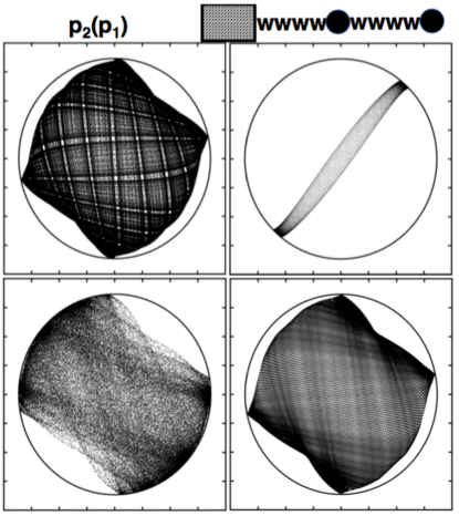
Figure 1: The top row shows $p_{2}(p_{1})$ projections for initial values $\{\ p^{2}\ \}=(11.6,0.4)$ at the left and $(6,6)$ at right. The bottom row shows $p_{2}(p_{1})$ projections for initial squared momenta of (12,0) at left and (0,12) at right. Runge-Kutta fourth-order integration with $dt=0.001$ and ${\cal H}=6$ are used in Figures 1-3. The bottom left projection represents chaos, with a Lyapunov exponent of 0.05. The other three do not. It appears that the combination (11.4,0.6) is chaotic with a Lyapunov exponent of order 0.003. The circles in Figure 1 represent the maximum momenta, $p^{2}=12$.

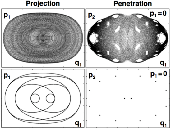
Figure 2: The left column shows phase-plane projections $p_{1}(q_{1})$ and the right column $p_{2}(q_{1})$ shows Poincaré sections $p_{2}(q_{1})$ with $p_{1}=0$. The initial momenta for the top row are $\{\ p^{2}\ \}=(12,0)$ and for the bottom row $(11.85,0.15)$. The top row is chaotic with $\lambda_{1}=0.05$ while the bottom row is close to a periodic orbit with $\lambda_{1}=0$. The top-row section suggests a “fat fractal” with infinitely-many tori threading through its perforations.

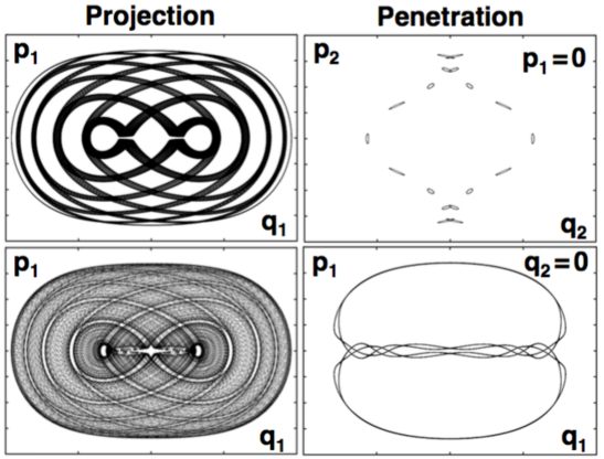
Figure 3: Here the top row initial momenta are $\{\ p^{2}\ \}=(11.5,0.5)$ and the motion is regular, with $\lambda_{1}=0$. The bottom row momenta are $(11.4,0.6)$ where chaos or its lack are still problematic, a region meriting more study. Here the left panels are projections while the right ones show Poincaré penetrations.

Aoki goes well beyond this interesting two-body problem. He considers a variety of $\phi^{4}$ chain problems in his provocative paper, considering the effects of symmetry and chaos on equilibrium temperature distributions, Lyapunov instability, and the pairing of the Lyapunov exponents. At present it is unknown whether or not the spectra become paired for all, or maybe “almost all” initial conditions. The $\phi^{4}$ model provides a surprisingly rich testbed for investigating Lyapunov instability.

Poincaré sections, two-dimensional cuts through the three-dimensional phase-density in its four-dimensional embedding space are shown at the right in Figure 2. The upper right section suggests a distribution resembling a ball of yarn with holes here and there, with these holes filled with periodic tori. Although far from ergodic the one-dimensional trajectory certainly explores most of the ${\cal H}=6$ region for this simplest of initial conditions where a single momentum variable carries all of the energy. Despite its two-spring simplicity the model’s quartic tethers are enough to bring out all the general features associated with Hamitonian chaos.

The Sections of Figure 3 hint at the “chains-of-islands” features typical of the boundaries separating regular and chaotic regions in sections of Hamiltonian chaos. A series of squared momenta in the neighborhood of (11.5,0.5) to 11.4,0.4) would make an interesting research investigation. Aoki also investigated a sightly more complex model with four degrees of freedom rather than just two. Let us consider it next.

II.2 Chaos with Four Bodies Subject to Periodic Boundary Conditions

A four-body periodic chain of $\phi^{4}$ particles has the Hamiltonian

$${\cal H}=(1/4)(q_{1}^{4}+q_{2}^{4}+q_{3}^{4}+q_{4}^{4})+(1/2)(p_{1}^{2}+p_{2}^{2}+p_{3}^{2}+p_{4}^{2})+$$

$$(1/2)[\ (q_{1}-q_{2})^{2}+(q_{2}-q_{3})^{2}+(q_{3}-q_{4})^{2}+(q_{4}-q_{1})^{2}\ ]\ .$$

With the implied periodic boundary conditions the special initial conditions ,

$$q_{1}=q_{2}=q_{3}=q_{4}=0\ ;\ p_{1}=p_{2}=-p_{3}=p_{4}=2\ ,$$

generate an interesting chaotic solution. It is symmetric. Consequently Particles 2 and 4 obey identical equations of motion. If as here the initial conditions have proper symmetry, identical dynamics results, with $q_{2}(t)=q_{4}(t)$ for all time. The motion corresponding to these conditions is chaotic. It likely generates a five-dimensional isoenergetic and chaotic “fat fractal”, in either six-dimensional or eight-dimensional phase space, $\Gamma=\{q,p\}$. Here the $\{q,p\}$ are the Cartesian coordinate-momentum pairs describing the system dynamics.

Figure 4 demonstrates the chaotic nature of that symmetric motion. It displays the convergence process $\langle\ \lambda_{1}(t)\ \rangle_{t\rightarrow\infty}\longrightarrow\lambda_{1}$ . The maximum Lyapunov exponent $\langle\ \lambda_{1}(t)\ \rangle$ is calculated by following two neighboring phase-space trajectories, the “reference” and a nearby “satellite” in either six or eight-dimensional phase space. The satellite trajectory is kept close to the reference by a rescaling of its phase-space separation from that reference at the end of every timestep :

$$|\ \Gamma_{r}(t+dt)-\Gamma_{s}(t+dt)\ |\longrightarrow\delta\ .$$

This condition is implemented by rescaling the separation to the fixed length $\delta$  :

$$\Gamma_{s}(t+dt)\longrightarrow\Gamma_{r}(t+dt)+\delta\frac{\ \Gamma_{s}(t+dt)-\Gamma_{r}(t+dt)\ }{|\ \Gamma_{s}(t+dt)-\Gamma_{r}(t+dt)\ |}\ .$$

The “local” “largest” Lyapunov exponent, $\lambda_{1}(t)$ for that timestep, is given in terms of the phase-space offsets before and after the rescaling operation :

$$|\ \delta\ |\propto e^{\lambda t}\longrightarrow\lambda_{1}(t)\equiv(1/dt)\ln[\ {\delta}_{\rm before}/\delta_{\rm after}\ ]\ .$$

Note well that what is here called “largest” is so only as a time average. The “largest” can at times actually be the smallest !

Figure 4 shows both six-dimensional and eight-dimensional cumulative time averages of the local largest Lyapunov exponent, as computed with fourth- and fifth-order Runge-Kutta integrators. The chaos of the $\phi^{4}$ dynamics guarantees that different integrators eventually generate different trajectory pairs and different local Lyapunov exponents. But the “global” long-time averages of the Lyapunov exponents are in statistical agreement with each other for any properly convergent integrator.

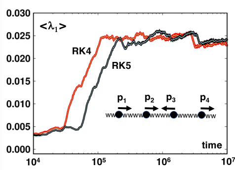
Figure 4: The cumulative “largest” Lyapunov exponent describing the four-particle chaos of a $\phi^{4}$ system with initial velocities $\{2,2,-2,2\}$ as computed in six-dimensional (thin lines) and eight-dimensional spaces ( thick lines ) using fourth-order and fifth-order Runge-Kutta integrators. For these simulations, with 10,000,000,000 timesteps $dt=0.001$, the reference trajectories agree precisely while the satellite trajectories show real, but negligibly small, differences.

Unlike many simple one-dimensional models augmenting harmonic chains the $\phi^{4}$ chains are tethered to fixed lattice sites by a quartic potential :

$$\{\ \ddot{q}_{i}=q_{i-1}-2q_{i}+q_{i+1}-q_{i}^{3}\ \}\ [\ {\rm Newtonian}\ \phi^{4}\ {\rm Model}\ ]\ .$$

The tethers kill the ballistic transmission of energy. Over wide ranges of energy and temperature $\phi^{4}$ chains exhibit Lyapunov instability ( exponential growth of small perturbations ) and Fourier conductivity, even for just a few particles. The initial conditions are not crucial so long as we choose them from a unique chaotic sea. With uniqueness long-time averages, either at or away from equilibrium conform to well-defined long-time averages. Until now investigations of small-system chaos have typically found a single chaotic sea for a given energy. This apparent simplicity could be misleading. In Aoki’s two-body $\phi^{4}$ model, pictured in Figures 1-3, $\lambda_{1}$ is 0.05 with the initial squared momenta $(12.0,0.0)$. For moderate run lengths at the same energy the initial momenta (11.4,0.6) lead instead to a smaller Lyapunov constant, $\simeq 0.003$. In their contribution Hofmann and Merker likewise suggest that the chaotic sea is not unique in a generalized Hénon-Heiles model with two degrees of freedom.

II.3 Fourier Heat Flow in Chaotic $\phi^{4}$ Systems

Hot and cold boundaries can be introduced into chaotic systems by adding temperature-dependent “thermostat” forces directing the kinetic temperatures of two or more particles’ mean values to their individual values $\{T_{i}\}$ :

$$\ddot{q}_{i}=F\longrightarrow\ddot{q}_{i}=F-\zeta\dot{q}_{i}\ {\rm with}\ \dot{\zeta}=\dot{q}_{i}^{2}-T_{i}\ [\ {\rm Nos\acute{e}-Hoover}\ \phi^{4}\ {\rm Model}\ ]\ .$$

The heat current that results reduces the dimensionality of the phase-space distribution from the equilibrium value of $2N$ for $N$ degrees of freedom by an amount roughly quadratic in the heat current. Reductions of the order of 50$\%$ have been obtained in steady-state heat flow simulations with a few dozen particles, one hot, one cold, and the rest purely Newtonianb4 .

These results follow from measurements of the spectrum of Lyapunov exponentsb4 . $\lambda_{1}(t)$ quantifies the local rate at which nearby pairs of phase-space trajectories separate. $\lambda_{1}+\lambda_{2}$ quantifies the rate at which triangles of phase-space trajectories grow or shrink, and $\lambda_{1}+\lambda_{2}+\lambda_{3}$ does this for tetrahedra. When such a sum of $n$ Lyapunov exponents has a positive average, overall growth of $n$-dimensional phase volumes occurs, and at the rate $\sum\lambda_{i\leq n}$. A negative sum indicates shrinkage onto a strange attractor with a dimensionality less than that of the full phase space.

In Hamiltonian systems growth and shrinkage necessarily cancel due to the time-reversibility of the motion equations. Nonequilibrium simulations with thermostats are typically time-reversible too. Both $\{\ \ddot{q}\ \}$ and the thermostat forces $\{\ -\zeta\dot{q}\ \}$ are even functions of the time. Nevertheless, in practice the greater abundance of compressive phase-space states causes symmetry breaking. The invariable shrinkage of the comoving phase volume onto a nonintegral-dimensional “fractal” strange attractor results. In the nonequilibrium case the spectrum of exponents is always shifted toward more negative values. This is the heat-based mechanical explanation of the Second Law of Thermodynamics.

III Hénon-Heiles’ Model

A more mathematically oriented paper by Timo Hofmann and Jochen Merkerb5 took Honorable Mention in the Snook Prize competition with their study of the Hénon-Heiles model in a four-dimensional Hamiltonian phase space :

$${\cal H}=(1/2)(p_{x}^{2}+p_{y}^{2}+x^{2}+y^{2})+x^{2}y-(y^{3}/3)\ [\ {\rm H\acute{e}non-Heiles}\ {\rm Model}\ ]\ .$$

Hénon-Heiles models are unsuited to conductivity or to manybody problems but still have considerable interest. Hofmann and Merker made a plausible argument for the coexistence of two chaotic seas for a generalized Hénon-Heiles model augmented by three quartic, three quintic, and four sextic terms in the four-variable generalized Hamiltonian.

Hofmann and Merker compared three versions of local Lyapunov exponents for their model and concluded that the Gram-Schmidt local exponents are not necessarily paired because their values depend upon the initial conditions. We decided to award their work an Honorable Mention in view of its interest and their exploration of a problem area quite different to Aoki’s. We congratulate all three men.

IV Epilogue and Moral

For Carol and me it was a challenge to reproduce some of the work of all the Snook Prize entries. It often takes real effort to dissipate the uncertainty characteristic of numerical chaos work. But by using reproducible “random number generators”, straightforward integrators, and careful descriptions of all the necessary initial conditions it is still possible to describe reproducible results, the sine qua non of physics. We are very grateful to Ken Aoki, Timo Hofmann, and Jochen Merker for their useful and interesting contributions, as well as the welcome input from several anonymous referees and colleagues.

V Acknowledgments

We are particularly grateful to Kris Wojciechowski for stimulating and overseeing this work and to Giancarlo Benettin, Carl Dettmann, Puneet Patra, Harald Posch, and Roger Samelson for their patient comments and suggestions regarding aspects of last year’s Snook Prizes. We very much appreciate the Institute of Bioorganic Chemistry of the Polish Academy of Sciences and the Poznań Supercomputing and Networking Center for their continued support of the Ian Snook Additional Prize.

References

- (1) Wm. G. Hoover and C. G. Hoover, “Instantaneous Pairing of Lyapunov Exponents in Chaotic Hamiltonian Dynamics and the 2017 Ian Snook Prizes”, Computational Methods in Science and Technology 23 (1), 73-79 (2017).
- (2) K. Aoki, “Symmetry, Chaos, and Temperature in the One-Dimensional Lattice Theory”, Computational Methods in Science and Technology (to appear, 2018).
- (3) K. Aoki and D. Kusnezov, “Lyapunov Exponents and the Extensivity of Dimensional Loss for Systems in Thermal Gradients”, Physical Review E 68, 056204 (2003).
- (4) Wm. G. Hoover and C. G. Hoover, Microscopic and Macroscopic Simulation Techniques - Kharagpur Lectures (World Scientific Publishers, Singapore, 2018), Section 10.8.
- (5) T. Hofmann and J. Merker, “On Local Lyapunov Exponents of Chaotic Hamiltonian Systems”, Computational Methods in Science and Technology (to appear, 2018).