Instability of particulate pipe flow

Abstract

We present linear stability analysis for a simple model of particle-laden pipe flow. The model consists of a continuum approximation for the particles two-way coupled to the fluid velocity field via Stokes drag (Saffman,, 1962). We extend previous analysis in a channel (Klinkenberg et al.,, 2011) to allow for the initial distribution of particles to be inhomogeneous and in particular consider the effect of allowing the particles to be preferentially located around one radius in accordance with experimental observations. This simple modification of the problem is enough to alter the stability properties of the flow, and in particular can lead to a linear instability at experimentally realistic parameters. The results are compared to the experimental work of Matas et al., 2004a and are shown to be consistent with the reported flow regimes.

1 Introduction

This paper is concerned with the wide issue of how particles affect the transition to turbulence in a pipe flow. Beside the fundamental interest of this canonical problem, several industrial sectors have seen a growing need to accurately measure flow rates or volume fractions in complex fluid mixtures flowing through pipes. Examples range from the precise determination of the volume fraction of oil in the oil-water-sand-gas mixture that is extracted from offshore wells, to needs in the food processing industry (Ismail et al.,, 2005), and flows of molten metal carrying impurities during recycling processes (Kolesnikov et al.,, 2011). Each of these examples requires dedicated flow metering technologies, most of which rely on a priori knowledge of the nature of the flow inside the pipe or the duct and in particular whether it is turbulent or not (Wang and Baker,, 2014). Though none of these examples could satisfactorily be modelled as a single fluid phase carrying one type of particles, the ideal problem of the particulate pipe flow constitutes one of their elementary building blocks. As such it is a good starting point from which to infer the basic mechanisms governing the transition to turbulence.

Adding particles opens a number of possibilities, associated with different physical mechanisms: particles can be buoyant or not, of different sizes and shapes, and also mono- or polydisperse. As a first step in studying the transition to turbulence in particulate pipe flows, we shall focus on the simpler case of neutrally buoyant, monodisperse spherical particles. Whether the effect of particles on the transition to turbulence in general is a stabilising or destabilising one mostly depends on the size and volume fraction of particles. Early experiments on the transition to turbulence in a pipe highlighted a critical volume fraction of particles below which they favoured the transition at a lower Reynolds number. At higher volume fractions than this critical value, by contrast, the effect was reversed (Matas et al.,, 2003). Recent numerical simulations based on accurate modelling of individual solid particles recovered this phenomenology (Yu et al.,, 2013).

The non-trivial nature of the influence of particles is further supported by the numerical study of individual perturbations introduced in a channel: whilst below a critical volume fraction, particles lower the critical energy beyond which perturbations triggered the transition to turbulence, the transition takes place longer after the perturbation was introduced in the presence of particles if the perturbation took the form of streamwise vortices (Klinkenberg et al.,, 2013). At high volume fraction, the critical energy was increased. Linear stability analysis in the same configuration provide a hint on the origin of this non-monotonous effect of volume fraction: they revealed the existence of an optimal stabilisation regime due to a maximum in the Stokes drag, when the particle relaxation time (i.e. the time for a particle at rest to accelerate to the velocity of the surrounding fluid), coincided with the period of the streamwise oscillation Klinkenberg et al., (2011).

Single phase pipe flow is governed by the a sole parameter, the nondimensional flow rate or Reynolds number. The problem remains linearly stable even at large Reynolds number (Meseguer and Trefethen,, 2003), and so the turbulence that is observed even at moderate flow rates (above $Re\simeq 2000$) must be initiated by finite amplitude disturbances. The inclusion of particles complicates this, and could even lead to linear instability.

Adding particles to the pipe flows raises the question of how particles shall be distributed in the pipe, at least in some initial state. While a homogeneous spatial distribution may first come to mind as the simplest possible, particles in pipe are known to aggregate near a specific radius greater than $65\%$ of the pipe radius (Segré and Silberberg,, 1962), that increases slowly with the Reynolds number. The underlying mechanism is driven by the radial variations of the lift force experienced by particles rotating in shear (Repetti and Leonard,, 1964). The dependence of the aggregation radius (often called the Segré-Silberberg radius) on the Reynolds number can be explained by means of asymptotic theory introducing the particle Reynolds number as the small parameter in the expression of the lift force (Schonberg and Hinch,, 1989; Hogg,, 1994; Asmolov,, 1999).

While this dependence is well recovered in experiments at moderate Reynolds numbers, a second equilibrium position appears at a lower radius (Matas et al., 2004a, ) for $Re>600$. Although this transition coincides with a change in the concavity of the radial profile of the lift force, the detailed mechanisms driving this effect remain to be found, and the authors left open the question of whether this equilibrium is stable or not. Han et al., (1999) note that the main effect of particle concentration on this phenomenology is to disperse the particle distribution around the equilibrium annulus. However, higher concentrations can also lead to the formation of trains of particles aligned with the stream Matas et al., 2004b . In the context of the transition to turbulence, the natural tendency of particles to aggregate around specific radii at different Reynolds numbers raises the question of the critical Reynolds at which these annuli of particles break-up and whether this break-up plays any role in the triggering of turbulence.

The variety of phenomena observed in particulate flows illustrates the numerous aspects of its transition to turbulence (starting with the difficulty of even distinguishing turbulent fluctuations from particle-induced ones). As such our purpose in the context of the pipe flow shall be limited to first step of investigating the linear stability of the particulate pipe flow to infinitesimal perturbations. Tackling this question requires the choice of a strategy to model particles (see Maxey, (2017) for a review on current methods). While the most accurate method consists of modelling particles as individual solids (Uhlmann,, 2005), this approach is the most computationally expensive and may not allow for consideration of a long enough pipe to cover long-wave instabilities. Cost-effective alternatives exist based on individual point-particle model that can incorporate various levels of complexity (one or two-way interaction, rotation of particles, particle interaction etc…). However, in the spirit of simplicity of this first step, we shall follow the even simpler option of modelling particles as a second fluid phase whose interaction with the fluid phase is limited to the drag forces that each phase exerts on the other (Saffman,, 1962; Klinkenberg et al.,, 2011) . Within this framework we address the questions of whether particulate pipe flow is stable for either homogeneous or inhomogeneous distributions of particles; which distributions of particles most adversely effect stability; and whether the distributions are realistic in comparison with experiments. The paper is organised as follow: in section 2, we shall introduce the model and the assumptions it relies as well as the numerical methods used. We shall then start by considering the simplest case of a homogeneous particle distribution in the pipe (section 3), before studying the linear stability of particles normally distributed around a radius, paying particular attention on how the standard deviation and the value of this radius influence the flow stability (section 4). We then compare our findings to the experiments of Segré and Silberberg, (1962) and Matas et al., 2004a (section 5), where localisation was observed before discussing the possible implications of our results for the transition to turbulence (section 6).

2 Model and governing equations

In order to avoid the heavy computational load cost incurred by when accounting for particles as individual solids, we describe the particulate flow using the “two-fluid” model first derived by Saffman, (1962). Particles are described as a continuous field rather than as discrete entities with a finite size. This model takes into account neither effects due to particle-particle interactions such as collisions or clustering, nor the deflection of the flow around the particles around particles. It is therefore valid for lower concentrations and in the limit where particles are sufficiently smaller than the characteristic scale of the flow.

We consider the flow of a fluid (density $\rho$, viscosity $\mu$) through a straight pipe with constant circular cross-section of radius $r_{0}$ and driven by a constant pressure gradient. The fluid carries particles of radius $a$. To describe the problem we adopt the model proposed by Saffman, (1962) and studied by Klinkenberg et al., (2011) in the context of channel flow. The particles are considered as a continuous field with spatially varying number density $N$, their motion coupled to the fluid solely via Stokes’ drag, $6\pi a\mu(\mathbf{u_{p}}-\mathbf{u})$. We take coordinates $(r,\theta,z)$ with respective velocities $\mathbf{u}=(u,v,w)$. Where relevant we distinguish those quantities associated with the particles from those associated with the fluid by means of a subscript $p$. After nondimensionalising by the centreline velocity, $U_{0}$, the pipe radius $r_{0}$ and the fluid density $\rho_{f}$ we have the equations

$$\partial_{t}\mathbf{u}+(\mathbf{u}\cdot\nabla)\mathbf{u}=-\nabla\mathbf{p}+\frac{1}{Re}\nabla^{2}\mathbf{u}+\frac{f}{SRe}(\mathbf{u_{p}}-\mathbf{u}),$$ (1)

$$\partial_{t}\mathbf{u_{p}}+(\mathbf{u_{p}}\cdot\nabla)\mathbf{u_{p}}=\frac{1}{SRe}(\mathbf{u}-\mathbf{u_{p}}),$$ (2)

$$\partial_{t}N=-\nabla\cdot(N\mathbf{u_{p}}),$$ (3)

$$\nabla\cdot\mathbf{u}=0.$$ (4)

We have non-dimensional Reynolds numbers $Re=U_{0}r_{0}/\nu$, dimensionless relaxation time $S=2a^{2}\rho_{p}/9r_{0}^{2}\rho_{f}$ and mass concentration $f=m_{p}/m_{f}$, the ratio of total mass of particles to total mass of fluid. These equations are augmented with an impermeable and no-slip boundary condition for the fluid

$$\mathbf{u}|_{r=1}=0$$ (5)

and a no penetration boundary condition for the particles

$$u_{p}|_{r=1}=0.$$ (6)

The stability of the flow is studied through the addition of a small perturbation to the steady solution ($\mathbf{U}=\mathbf{U}_{p}=(1-r^{2})\hat{\mathbf{z}}$)

$$\mathbf{u}=\mathbf{U}+\mathbf{u}^{\prime},\;\;\mathbf{u_{p}}=\mathbf{U}+\mathbf{u_{p}}^{\prime},\;\;p=P+p^{\prime},\;\;N=N_{0}+N^{\prime}.$$

Linearising equations (1) - (4) around this base state and dropping the primes gives

$$\partial_{t}\mathbf{u}+\mathbf{U}\cdot\nabla\mathbf{u}+\mathbf{u}\cdot\nabla\mathbf{U}=-\nabla\mathbf{p}+\frac{1}{Re}\nabla^{2}\mathbf{u}+\frac{f}{SRe}(\mathbf{u_{p}}-\mathbf{u}),$$ (7)

$$\partial_{t}\mathbf{u_{p}}+\mathbf{u_{p}}\cdot\nabla\mathbf{U}+\mathbf{U}\cdot\nabla\mathbf{u_{p}}=\frac{1}{SRe}(\mathbf{u}-\mathbf{u_{p}}),$$ (8)

$$\partial_{t}N=-N_{0}\nabla\cdot\mathbf{u_{p}}-\mathbf{u_{p}}\cdot\nabla N_{0}-\mathbf{U}\cdot\nabla N,$$ (9)

$$\nabla\cdot\mathbf{u}=0.$$ (10)

The boundary conditions for the perturbation are the same as for the full flow.

2.1 Linear stability

Given the streamwise and azimuthal invariance of the problem, we consider perturbations of the form

$$g(r,\theta,z,t)=\sum_{n=0}^{N}g_{n}T_{n}(r)\exp\{i((\alpha z+m\theta-\omega t)\},$$ (11)

where $T_{n}$ is the $n^{th}$ Chebyshev polynomial and $g$ is any of the fields of interest, with corresponding coefficients $g_{n}$ in the expansion. Substituting this into equations (7)-(10) and boundary conditions (5) and (6) leads, after collocation, to a generalised eigenvalue problem

$$i\omega\mathbf{A}\mathbf{\phi}=\mathbf{B}\mathbf{\phi}$$ (12)

which can be solved using LAPACK.

The code was validated for the case of non-particulate pipe flow against Meseguer and Trefethen, (2003) and for particulate flow in a channel against Klinkenberg et al., (2011). With 100 Chebychev polynomials, the relative error remains below $10^{-7}$ for the various tested combinations of values of $\alpha\leq 1$, $m\leq 1$ and $Re<10^{4}$. With the addition of particles, the precision dropped to $10^{-6}$ for $S=10^{-3}$ and down to $10^{-5}$ for $S=0.1$, with as many as 200 polynomials.

To further test all cases, we created a linear simulation code based on the non-particulate DNS code of Willis, (2017). This code uses Fourier-modes in the axial and azimuthal directions, and finite differences radially. This allowed us to check the leading eigenvalue of each different Fourier mode for any given configuration. Accuracy between the methods was confirmed to be within 1%.

3 Uniform particle distribution

Previous work on this model (Klinkenberg et al.,, 2011) has made the assumption that the initial distribution of particles is uniform throughout the domain. This simplifies the governing equations as $\nabla N_{0}=0$, removing terms and decoupling equation (9) from the rest of the problem.

3.1 Modified eigenvalue spectrum

The addition of uniformly distributed particles does not lead to large changes in the stability problem of pipe flow. Figure 1 compares the eigenvalue spectra of the particulate and non-particulate problems for one typical case. The overall shape of the spectrum is qualitatively unchanged, maintaining three branches, the location of the leading eigenvalue being at the tip of the ‘P’-branch (Mack,, 1976) .

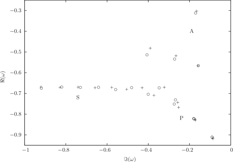
Figure 1: Eigenvalue spectra for the generalised eigenvalue problem (12) for $Re=1000$, $S=10^{-3}$, $\alpha=1$, $f=0.1$. The classical single phase eigenvalues are marked ‘$+$’ while the eigenvalues for the particulate flow are marked ‘$\circ$’. The three branches of the eigenspectrum are labelled $A$, $P$ and $S$ in accordance with the notation of Mack, (1976)

We quantify the change in the eigenvalue spectrum by tracking the normalised growth rate

$$\lambda^{\prime}_{p}(Re,\alpha,m,f,S)=\frac{\Im\{\omega_{p}(Re,\alpha,m,f,S)\}}{\Im\{\omega_{f}(Re,\alpha,m)\}},$$ (13)

where $\omega_{p}$ and $\omega_{f}$ are the leading eigenvalues in the particulate and non-particulate problems. From the definition (11) the growth rate is the imaginary part of the eigenvalue. As the pure-fluid problem is linearly stable (meaning $\Im\{\omega_{f}\}$ is always negative), $\lambda_{p}^{\prime}>1$ is indicative of the particles stabilising the flow while $\lambda_{p}^{\prime}<1$ corresponds to them destabilising the flow. The critical value $\lambda_{p}^{\prime}=0$ would indicate the particulate problem crossing the neutral stability threshold, however this was never observed for any parameter combination with a uniform distribution of particles.

Parameter space is simplified by the observation that the role of $f$, the concentration, seems to be secondary. Figure 2 shows $\lambda^{\prime}_{p}$ as a function of $f$ and in all cases the concentration serves simply to amplify the underlying result almost linearly. Consequently, in the analysis of the uniform particle distribution problem we fix $f=0.01$ in the knowledge that trends could be exacerbated further by increasing the quantity.

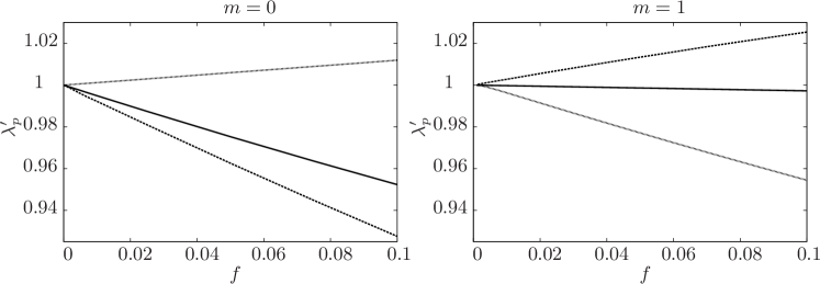
Figure 2: Normalised growth rate, $\lambda_{p}^{\prime}$, as a function of $f$ for $S=10^{-3}$ (line), $S=10^{-2}$ (dots), $S=10^{-1}$ (dashed) with $Re=1000$, $\alpha=1$. In all cases examined, $\lambda_{p}^{\prime}$ is very close to being proportional to $f$, suggesting that this parameter simply serves to amplify the underlying result linearly.

3.2 Influence of Stokes number

Stokes number reflects the size of the particles. It is most easily understood in terms of its limiting values. In the ballistic limit, $S\rightarrow\infty$ the large particles become independent of the flow. In the other extreme, $S\rightarrow 0$, the particles are passive tracers. In neither case do the particles unduly influence the flow. In the former, they fully decouple and one recovers the pure fluid results. In the latter case, the particles act as one with the fluid, only changing the effective density of the total suspension. This rescales the effective Reynolds number as $Re^{\prime}=(1+f)Re$ (Klinkenberg et al.,, 2011).

In between these two extreme limits, non-trivial changes occur to the leading eigenvalue. For $m=0$ the behaviour is readily described. In figure 3 (left), $\lambda_{p}^{\prime}$ smoothly varies from less stable ($\lambda_{p}^{\prime}\simeq 0.995$ for $S=0$) to unaffected ($\lambda_{p}^{\prime}=1$ for $S\rightarrow\infty$), it does not do so monotonically. In particular it initially decreases the stability of the flow, then over stabilises the flow past the level of a pure fluid before it subsides to the particle-free result. This occurs for all $Re$ and $\alpha$ considered.

This result is clarified further by fixing $S$ and varying $Re$, as in figure 4. For low values of $S$ (here $10^{-3}$) the stability remains effectively unchanged at these Reynolds numbers with the particles remaining as passive tracers. For large Stokes number ($S=0.1$) there is some variation of $\lambda_{p}^{\prime}$ with $Re$, but it is relatively benign as the particles decouple from the flow. It is only at intermediate Stokes number ($S=0.01$) that we see nontrivial behaviour for moderate Reynolds number.

The case of $m=1$ is more complex (figure 3, right). The limiting cases of very large or very small $S$ still behave as expected (though now even smaller values of $S$ must be considered to recover the limiting case) but the intermediate behaviour is more involved. The particles can either stabilise or destabilise the flow depending on the precise parameters chosen. For a given $Re$ and $\alpha$, increasing $S$ can lead to the flow switching repeated between one and the other.

We conclude this section by noting that the simple behaviour for $m=0$ suggests we may be able to isolate some simple behaviour. To identify the region in which particles have the most significant effect on the flow, we define $S^{m}$ to be the Stokes number for which the flow is most destabilised and $\lambda_{p}^{\prime}$ is minimised. Least squares fitting suggests a clear scaling of $S_{m}$ with both $Re$ and $\alpha$ as shown in figure 5. While the effect is somewhat unsurprisingly amplified at larger Reynolds number, it mostly concerns longer wavelengths and remains limited in amplitude in all cases (we never found an increase of growthrate more that 2% higher than the single fluid case).

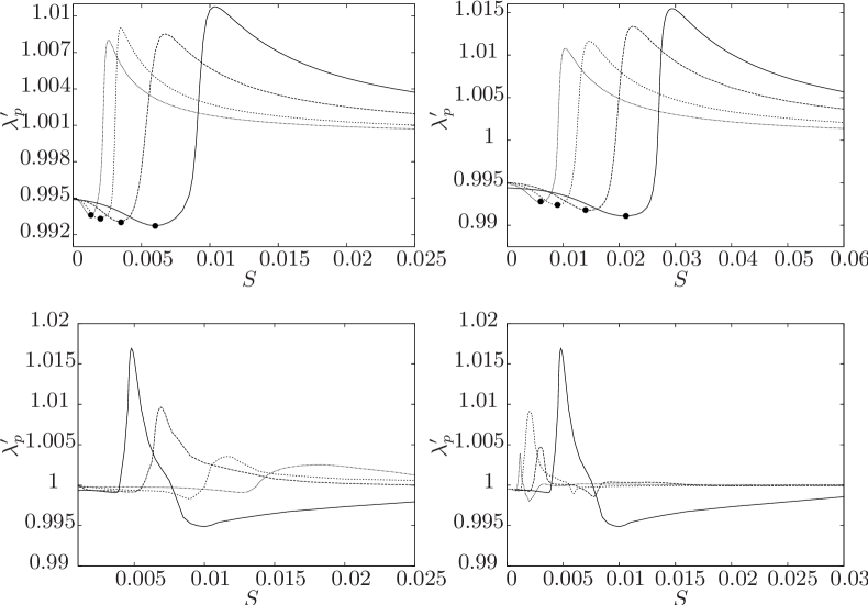
Figure 3: Normalised leading growthrate, $\lambda_{p}^{\prime}$, as a function of $S$ while keeping $f=0.01$. The top row is $m=0$, the bottom is $m=1$. In all cases we see that for low Stokes number we recover the result of a single fluid, albeit of larger effective density. For large $S$ the particulate eigenvalue tends towards that of the non-particulate case and hence $\lambda_{p}^{\prime}\rightarrow 1$. For $m=0$, in each case there is a clearly defined $S^{m}$ (marked $\bullet$) for which $\lambda^{\prime}_{p}$ is minimised and the flow is least stable. Left: Fixed $\alpha=2$ and $Re=1000$ (line), $3000$ (dashed), $10000$ (short dashed), $20000$ (dots). There is no qualitative change in behaviour, but the Stokes number for which the effect of the particles changes from destabilising to stabilising reduces with $Re$. Right: Fixed $Re=1000$ and $\alpha=0.2$ (line), $0.4$ (dashed), $1$ (short dashed), $2$ (dots). Again there is no qualitative change with $\alpha$ but the region of $S$ where the effect changes from destabilising to stabilising decreases with $\alpha$.

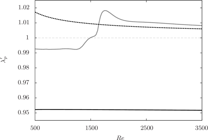
Figure 4: Normalised leading growthrate, $\lambda_{p}^{\prime}$ for $m=0$ as a function of $Re$, for $S=10^{-3}$ (line), $S=10^{-2}$ (dots), $S=10^{-1}$ (dashed) with $f=0.01$, $\alpha=1$. While the largest and smallest values of $S$ present straightforward, monotonic behaviour, the intermediate $S=0.01$ presents non-trivial variation with Reynolds number.

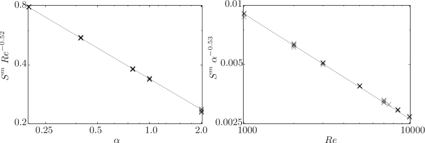
Figure 5: The variation $S^{m}$ with $Re$ and $\alpha$. The data can be collapsed down on to a single line by using an appropriate rescaling. Upper: $S^{m}Re^{-0.52}$ (exponent given to two significant figures) as a function of $\alpha$. The collapsing of the data onto close to a single line suggests $S^{m}\propto Re^{0.52}$. Lower: $S^{m}\alpha^{-0.53}$ as a function of $Re$. The data again collapses onto a single line, though not as cleanly as for the scaling in $Re$. Nonetheless, this suggests $S^{m}\propto\alpha^{-0.53}$.

4 Nonuniform particle distributions

There is nothing inherent in the model which requires the initial distribution of particles to be uniform. Relaxing this assumption allows to us to consider a more general problem, albeit at the cost of including all terms in the linearised equations (7)-(10). As discussed in the introduction, experimental work suggests that for low to moderate Reynolds numbers particles congregate at a particular radius forming an annulus from their distribution centred in the region $r=0.5-0.8$. In this section we capture the essence of this by considering distributions of the form

$$N_{0}(r)=\tilde{N}\exp\{-(r-r_{d})^{2}/2\sigma^{2}\},$$ (14)

with $\tilde{N}$ chosen such that $\int_{0}^{1}N(r)rdr=1$.

Throughout this section we keep fix $S=10^{-3}$, $f=0.1$ and $m=1$ to reduce the set of parameters being considered. The first two of these is consistent with experimentally realisable parameters (see section 5) while $m=1$ is the only azimuthal wavenumber for which we observed instability.

4.1 The onset of instability

As soon as the assumption of uniform particle distribution is relaxed we see a linear instability occurring. Figure 6 shows the leading eigenvalues for two different localised distributions of particles compared with the uniform distribution result. Whereas the latter of these remains stable for all $Re$, the two non-uniform distributions are unstable. Of particular note is that in both cases we see instability for moderate Reynolds number, but not for either high or low $Re$. This initially surprising observation that the flow re-stabilises as $Re$ increases is a recurrent observation. For very large $Re$, there is no coupling between the fields and everything is stable. For low $Re$, diffusion dominates and imposes stability. Only in the middle is instability feasible.

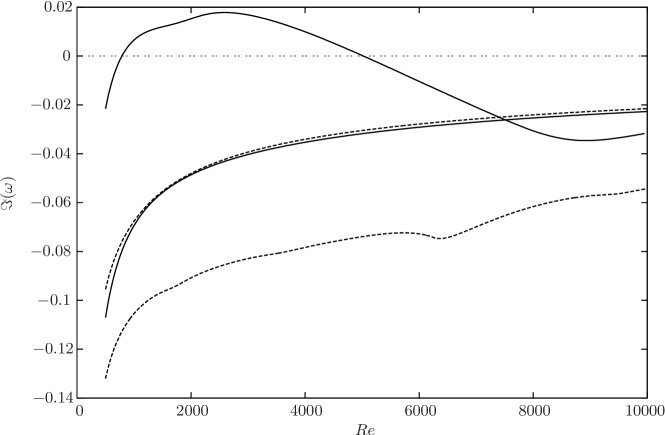
Figure 6: The leading eigenvalue for uniform (solid) and non-uniform particle distributions, centred at either $r=0.6$ (dashed) or $r=0.7$ (dotted). The uniform distribution is stable for all $Re$, but both the non-uniform distributions are unstable for a range of $Re$. For higher $Re$ the leading eigenmode switches between A and P branches for both non-uniform distributions at the point where dashed and solid lines meet on the graph.

For higher $Re$, after the flow has restabilised we observe there is a switching of the leading eigenmode (at around $Re=6000-8000$) after which the dominant eigenmode appears to be the same as for the uniform problem. Closer examination of the eigenvalue spectrum (figure 7) reveals that for an unstable configuration, the leading eigenvalue is now in the P-branch of the spectrum, rather than the A-branch as in the case of both the non-particulate and uniformly distributed problems.

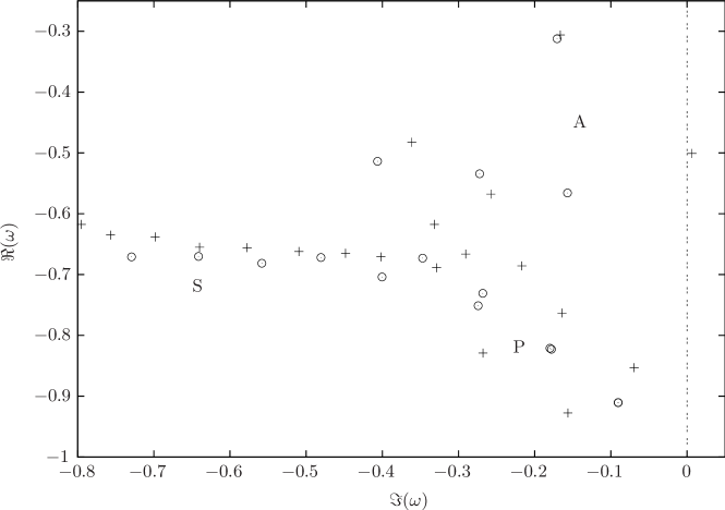
Figure 7: Eigenvalue spectra for the non-particulate ($\circ$) and particulate cases ($+$). In both cases $Re=1000$, $\alpha=1$ and $m=1$ while the particles were non-uniformly distributed with $f=0.1$, $r_{d}=0.6$ and $\sigma=0.1$.

The reason for the switching of branches becomes clear as soon as we examine the eigenmodes associated with the two eigenvalues. In figure 8 the leading eigenmodes of the two branches are plotted. The overall shape is relatively insensitive to the distribution of particles, but the modes of the two branches are primarily active in different parts of the pipe. For the A-branch, the eigenmode is localised to a relatively central part of the domain (centred at $r\approx 0.3$), while the P-branch mode is located nearer the edge of the pipe ($r\approx 0.7$). It is unsurprising that when the particle distribution is centred near this outer location, these are the eigenmodes that are primarily excited.

As well as only being unstable for a finite range of $Re$, the flow is also only unstable for a finite range of $\alpha$ (figure 9). For both small and large wavenumber disturbances the flow is stable. The latter is to be expected due to the stabilising influence of viscosity, but it is important to note the instability exists at very moderate wave numbers for which the model is expected to be valid.

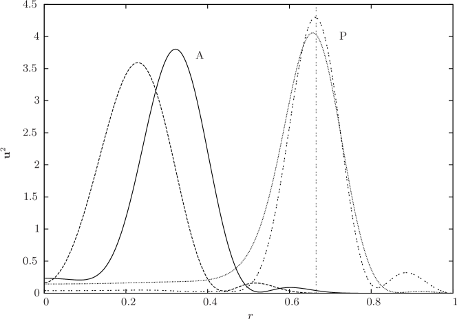
Figure 8: The distribution of the fluid energy in the leading eigenmodes. The two that peak on the left are the leading A branch modes for the non-particulate (solid line) and particulate case (dashed). The leading P modes peak on the right with the non-particulate case being double-dashed and the particulate profile dotted. For the particulate case the particles are non-uniformly distributed with $Re=1000$, $m=1$, $f=0.1$, $S=10^{-3}$, $r_{d}=0.7$ and $\sigma=0.1$. The vertical line is at $r_{d}^{*}=0.666$.

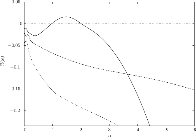
Figure 9: The leading growthrates for $Re=1000$, $m=1$, $f=0.1$, $S=10^{-3}$, $r_{d}=0.65$ and $\sigma=0.1$. Instability ($\Im\{\omega\}>0$) only occurs for a finite range of $\alpha$, with the flow being stable to both long and short wavelength disturbances.

4.2 Effect of the radial distribution of particles

The exact location where the particle annulus ($r_{d}$) is centred, and how sharply the distribution peaks around this location, plays an important role in determining whether the flow becomes unstable or not. By searching over $\alpha$ we can trace out neutral stability contours in $Re-r_{d}$ space for differing values $\sigma$ (figure 10, upper). The enclosed regions are unstable and we see that all the contours are indeed closed. The fact that there is a minimum/maximum value of $Re$ for which the flow is unstable is consistent with our earlier observations, while the fact that there are bounds on the value of $r_{d}$ supports the thesis of needing to excite the P-branch in order to destabilise the flow. We note that for all values of $\sigma$ the curves are concentric and the broadest range of unstable $Re$ occurs when $r_{d}$ is in the region $0.6-0.7$.

We track the maximum and minimum values of $r_{d}$ for which instability exists in figure 10 (lower). By doing so we arrive at a minimum degree of localisation required to trigger instability, corresponding to $\sigma^{*}=0.111$, for which the particle distribution must be centred at $r_{d}^{*}=0.666$.

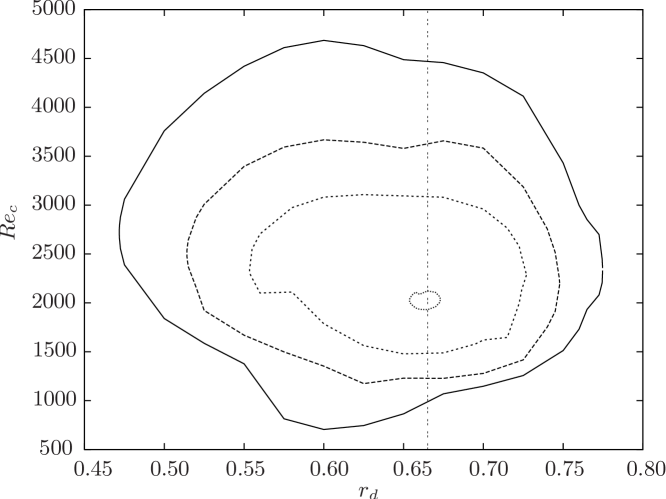
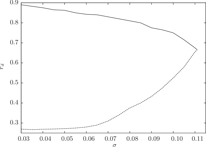
Figure 10: Upper: Contours of neutral stability in $Re-r_{d}$ space for values of $\sigma=0.110$, $0.105$, $0.100$ and $0.095$ from innermost to outermost. In each case, the enclosed region is the unstable region. That all the contours are closed indicates there is a maximum/minimum value of both $Re$ and $r_{d}$ for which flow is unstable. Lower: The maximum (solid)/minimum (dashed) values of $r_{d}$ for which the flow becomes unstable as $\sigma$ is varied, searching across all $Re$. There is a maximum value of $\sigma$ beyond which instability isn’t possible.

5 Relevance to experimental configurations

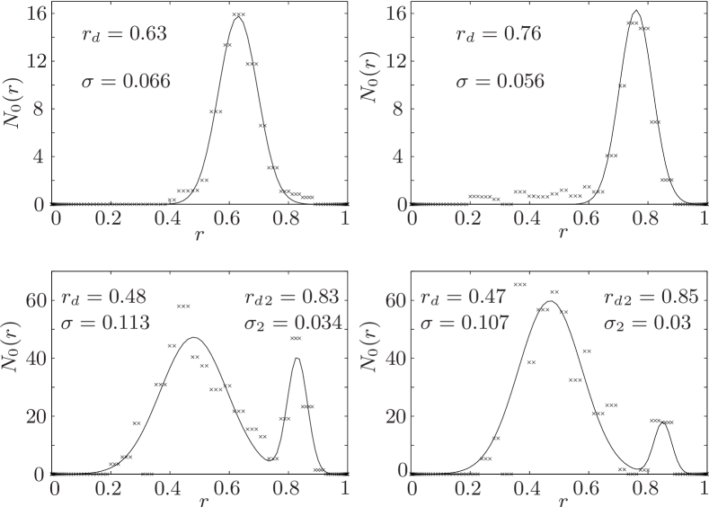
Figure 11: Particles concentration as a function of the radius. The crosses show the experimental results of Matas et al., 2004a while the lines are our fitted distributions. For the top row ($Re=67$ (left) and $Re=350$ (right)) a single gaussian was fitted for each case, centred at $r_{d}$ and of width $\sigma$. For the bottom row ($Re=1000$ (left) and $Re=1650$ (right)) each set of data was fitted with the sum of two gaussians of the given locations and widths.

		$\Im\{\omega\}$
$Re$	$S$	particle free	discontinuous	continuous
$67$	$2.743\times 10^{-3}$	$-0.58409$	$-0.56033$	$-0.55828$
$350$	$2.743\times 10^{-3}$	$-0.14605$	$-0.16606$	$-0.17752$
$1000$	$7.689\times 10^{-4}$	$-0.091143$	$-0.10480$	$-0.10635$
$1650$	$7.689\times 10^{-4}$	$-0.074771$	$-0.094478$	$-0.099083$

Table 1: Comparison of leading eigenvalues for the linear stability problem obtained in the cases of no particles, with particles distributions experimentally found by Matas et al., 2004a (see figure 11), and with particles distributed with closest Gaussian fits to the experimental data (the parameters given in figure 11). In each case the eigenvalues are given for $m=1$ and $\alpha=1$.

Matas et al., 2004a explores the effect of adding particles to pipe flow. As with other experimental work they report the clustering of particles at preferential radii that motivates this study but they do not report evidence of a linear instability. In this section we analyse the configurations observed by Matas et al., 2004a and show that our numerical results are consistent with the experiments - that is that we find the configurations to be linearly stable.

In the experimental work, four configurations of particles are explicitly given (figure 11) corresponding to $Re=67$, $350$, $1000$ and $1650$ (left to right, top to bottom). At low $Re$ the particles all cluster at a single radius consistent with Segré and Silberberg, (1962). As the $Re$ is increased, two preferential radii emerge and coexist. We capture these distributions within the linear stability analysis with two approaches. Firstly we fit either one or two Gaussian distributions through the data using least squares. These fits and the corresponding fitting parameters are those given in 11. Secondly, we use the raw data to give a discontinuous distribution with the $N(r)$ being taken as constant between data points.

In table 1 we give the growth rates of the leading eigenvalues for non-particulate flow, particles distributed continuously and particles distributed discontinuously for the different configurations reported by Matas et al., 2004a. For $Re=67$ both distributions of particles reduce the stability of the flow, but not so far as to make it unstable. For the higher values of $Re$, the particles in fact stabilise the flow further. These effects apply for both the Gaussian and discontinuous particle distributions and all growth rates agree to within at most $7\%$, much less than the discrepancy with the non-particulate case. We conclude that within the set of cases experimentally studied, our numerical results are fully consistent with the observations.

6 Conclusions and discussion

We have presented a very simple model for particulate pipe flow. Although this model has been examined before in plane shear flow (Saffman,, 1962; Klinkenberg et al.,, 2011), it has only been done in the context of an initially uniform particle distribution. In that previous work, the flow has always remained stable and here this is observed for pipe flow too. We are able to track the curves in parameter space for which the flow becomes most effected by the presence of particles, but it does always remain stable.

Relaxing the assumption of uniformly distributed particles, and allowing for the experimentally observed situation of particles arranged preferentially in an annulus is sufficient to induce linear instability in the flow for certain ranges of parameter. In particular, the flow is only ever unstable for intermediate Reynolds numbers, restabilising as $Re$ is increased further. This in-between regime is sandwiched between low $Re$ flows dominated by viscous diffusion and high $Re$ flows where the two phase decouple. The instability also only exists at intermediate axial wavenumbers. This avoids both the small length scale disturbances which violate the assumptions of the model and also the large (axial) scale disturbances which must test any assumption of axial independence of the base state.

The linear instability appears strongest when the annulus of particles is centred at $r_{d}\approx 0.65$ both in terms of this being the location where the smallest degree of localisation is needed for instability and being closely correlated with the widest band of unstable $Re$ for stronger localisation. This is particularly important as experimental work suggests that particles naturally congregate at this radius. The experimental work done to date on transitional particulate pipe flow (Matas et al.,, 2003; Matas et al., 2004a, ) has all been within the region of parameter space that this study has found to be linearly stable and so is entirely consistent with this.

That linear instability is feasible even within such a simple framework highlights the complexities of the problem and reveals that very different transition scenarios can be at play within the broader problem of particulate pipe flow. We do not submit this as a full explanation for the transition problem not least because it is possible that some of the excluded physics has a stabilising effect on the flow. In particular, the inertial mechanisms driving the particles to form into an annulus could be expected to act as a stabilising influence. Instead we suggest that the formation of an annulus of particles could be a key step in the onset of turbulence for certain, experimentally relevant parametric configurations of the problem.

7 Acknowledgements

AR is supported by TUV-NEL. CCTP is partially supported by EPSRC grant No. EP/P021352/1 . AP acknowledges support from the Royal Society under the Wolfson Research Merit Award Scheme (Grant WM140032). We thank Ashley Willis for use his code as well as useful discussions on adapting it.

References

- Asmolov, (1999) Asmolov, E. S. (1999). The inertial lift on a spherical particle in a plane poiseuille flow at large channel reynolds number. J. Fluid Mech., 381:63–87.
- Han et al., (1999) Han, M., Kim, C., Kim, M., and Lee, S. (1999). Particle migration in tube flow of suspensions. J. Rheol., 43:1157–1174.
- Hogg, (1994) Hogg, A. J. (1994). The inertial migration of non-neutrally buoyant spherical particles in two-dimensional shear flows. J. Fluid Mech., 272:285–318.
- Ismail et al., (2005) Ismail, I., Gamio, J., Bukhari, S., and Yang, W. (2005). Tomography for multi-phase flow measurement in the oil industry. Flow Measurement and Instrumentation, 16(2):145 – 155. Tomographic Techniques for Multiphase Flow Measurements.
- Klinkenberg et al., (2011) Klinkenberg, J., de Lange, H., and Brandt, L. (2011). Modal and non-modal stability of particle-laden channel flow. Physics of Fluids (1994-present), 23(6):064110.
- Klinkenberg et al., (2013) Klinkenberg, J., Sardina, G., De Lange, H., and Brandt, L. (2013). Numerical study of laminar-turbulent transition in particle-laden channel flow. Physical Review E, 87(4):043011.
- Kolesnikov et al., (2011) Kolesnikov, Y., Karcher, C., and Thess, A. (2011). Lorentz force flowmeter for liquid aluminum: Laboratory experiments and plant tests. Metallurgical and Materials Transactions B, 42(3):441–450.
- Mack, (1976) Mack, L. M. (1976). A numerical study of the temporal eigenvalue spectrum of the blasius boundary layer. Journal of Fluid Mechanics, 73(3):497–520.
- Matas et al., (2003) Matas, J.-P., Morris, J. F., , and Guazzelli, E. (2003). Transition to turbulence in particulate pipe flow. Phys. Rev. Lett., 90:014501.
- (10) Matas, J.-P., Morris, J. F., , and Guazzelli, E. (2004a). Inertial migration of rigid spherical particles in poiseuille flow. J. Fluid Mech., 515:171.
- (11) Matas, J.-P., V., G., Morris, J. F., and Guazzelli, E. (2004b). Trains of particle at finite reynolds number pipe flow. Phys. Fluids, 16(11):4192–4195.
- Maxey, (2017) Maxey, M. (2017). Simulation methods for particulate flows and concentrated suspensions. Annual Review of Fluid Mechanics, 49(1):171–193.
- Meseguer and Trefethen, (2003) Meseguer, A. and Trefethen, L. N. (2003). Linearized pipe flow to reynolds number 10 7. Journal of Computational Physics, 186(1):178–197.
- Repetti and Leonard, (1964) Repetti, R. V. and Leonard, E. F. (1964). Segré–silberberg’s annulus formation: a possible explanation. Nature, 203:1346–1348.
- Saffman, (1962) Saffman, P. G. (1962). On the stability of a laminar flow of a dusty gas. Journal of Fluid Mechanics, 13(01):120–128.
- Schonberg and Hinch, (1989) Schonberg, J. A. and Hinch, E. J. (1989). Inertial migration of a sphere in poiseuille flow. J. Fluid Mech, 203:517–524.
- Segré and Silberberg, (1962) Segré, G. and Silberberg, A. (1962). Behaviour of macroscopic rigid spheres in poiseuille flow part 2.: Experimental results and interpretation. J. Fluid Mech., 14:136–157.
- Uhlmann, (2005) Uhlmann, M. (2005). An immersed boundary method with direct forcing for the simulation of particulate flows. Journal of Computational Physics, 209(2):448 – 476.
- Wang and Baker, (2014) Wang, T. and Baker, R. (2014). Coriolis flowmeters: a review of developments over the past 20 years, and an assessment of the state of the art and likely future directions. Flow Measurement and Instrumentation, 40:99 – 123.
- Willis, (2017) Willis, A. P. (2017). The Openpipeflow Navier–Stokes solver. SoftwareX, 6:124–127.
- Yu et al., (2013) Yu, Z., Wu, T., Shao, X., and Lin, J. (2013). Numerical studies of the effects of large neutrally buoyant particles on the flow instability and transition to turbulence in pipe flow. Phys. Fluids, 25:043305.