Generative models for local network community detection

Abstract

Local network community detection aims to find a single community in a large network, while inspecting only a small part of that network around a given seed node. This is much cheaper than finding all communities in a network. Most methods for local community detection are formulated as ad-hoc optimization problems. In this work, we instead start from a generative model for networks with community structure. By assuming that the network is uniform, we can approximate the structure of unobserved parts of the network to obtain a method for local community detection. We apply this local approximation technique to two variants of the stochastic block model. To our knowledge, this results in the first local community detection methods based on probabilistic models. Interestingly, in the limit, one of the proposed approximations corresponds to conductance, a popular metric in this field. Experiments on real and synthetic datasets show comparable or improved results compared to state-of-the-art local community detection algorithms.

I Introduction

Networks are a convenient abstraction in many different areas, such as social sciences, biology, and the world wide web. A common structure in these real-world networks is a community, a group of nodes that are tightly connected and often share other properties, for example, biological function in a protein interaction network.

Imagine that you are trying to find such a community of nodes in a network. If the network is very large, it becomes too expensive to look at all nodes and edges in the network. Therefore local methods are needed. Local community detection aims to find only one community around a given set of seed nodes, by relying on local computations involving only nodes relatively close to the seed (Kloumann and Kleinberg, 2014; Andersen et al., 2006); in contrast to global community detection, where all communities in a network have to be found.

For global community detection, it is possible to treat the problem of finding all communities in a network as a probabilistic inference problem. This puts global community detection on a solid foundation, and makes it clear what a community is, and how these communities manifest in the network structure.

But most algorithms for local community detection operate by optimizing an ad-hoc objective function such as conductance (Andersen et al., 2006; Yang and Leskovec, 2012; Li et al., 2015).

In this paper we will fill this gap, and propose a probabilistic model for local community detection. Our contributions can be summarized as follows:

1. We introduce an approximation technique for using global models to perform local community detection.

2. We introduce the first method for local community detection based on a generative model by using this approximation.

3. We propose two algorithms for local community detection, based on approximations of the stochastic block model and of the degree-corrected stochastic block model.

4. We provide a probabilistic interpretation of conductance, as limit behavior of the approximate degree-corrected stochastic block model.

5. We show that the approximate stochastic block model is a highly competitive algorithm, which outperforms the state-of-the-art on three of five real life benchmark datasets.

I.1 Related work

I.1.1 Local community detection

Local network community detection methods have largely focused on optimizing conductance, which is a measure of the quality of a graph cut. Empirically, conductance has been shown to be a good quality metric for communities in real-world networks (Yang and Leskovec, 2012), in the sense that real-world communities often have a higher conductance than other sets of nodes.

Because community detection is computationally hard (Fortunato, 2010; Shi and Malik, 2000), several different heuristics have been developed. A common approach is to use spectral partitioning, which involves finding the dominant eigenvector of a random walk kernel. Andersen et al. (2006) showed that communities with a good conductance can be computed efficiently in this way. In their method nodes are added to the community in order of decreasing personalized pagerank score, and the community along this ‘sweep’ with the highest conductance is returned. Computing this personalized pagerank is a global operation, but efficient local approximations are possible, that only involve nodes near the seed.

Several variants of this sweep method have been proposed. Kloster and Gleich (2014) propose an alternative to the personalized pagerank score, based on the heat kernel instead of random walks. Yang and Leskovec (2012) propose to find the first local optimum of conductance instead of a global optimum. Other heuristics involve trying to find multiple pagerank-like vectors and restarting the method from different neighborhoods around the seed (Li et al., 2015).

However, being based on graph cuts, a good conductance is often achieved by cutting a network into roughly equal-sized parts, which is undesirable. To limit the size of communities, a cut-off on the personalized pagerank score can be used (Andersen et al., 2006); also, variations of the sweep methods have been proposed that stop at earlier local optima (Yang and Leskovec, 2012).

I.1.2 Global community detection

Many different global community detection methods have been developed for different classes of networks and different community structures. For a complete overview, we refer the reader to the surveys by Fortunato (2010); Xie et al. (2013).

Here we focus on probabilistic models for global community detection. The simplest are the stochastic block models (Paul W. Holland, 1983; Carolyn J. Anderson, 1992), which partition the nodes into communities, with varying probabilities of edges. These block models produce networks that are very different than real networks, in particular, the distribution of degrees is very different. To more accurately model the node degrees, Karrer and Newman (2011) have proposed the degree-corrected stochastic block model (DC-SBM). In this model, they add an extra parameter to each node, which controls the likelihood of edges to that node, and hence the node’s degree. This extra complexity comes at the cost of making the model more difficult to fit, and so degree correction might not be appropriate for all networks (Yan et al., 2014).

An issue with the stochastic block model is that the number of communities has to be fixed because with more communities there are more parameters in the model, which makes it impossible to compare likelihoods. The Infinite Relational Model (Kemp et al., 2006) solves this problem by assuming an infinite number of communities in combination with a Chinese restaurant prior over community structures.

The model of Newman and Leicht (2007) goes one step further, and has a parameter for each combination of node and community, indicating the likelihood of edges from nodes in that community to a particular other node. This is similar to models based on non-negative matrix factorization (Psorakis et al., 2011; Ball et al., 2011). These more complex models allow for nodes to be in more than one community.

Aside from these flat models, also hierarchical models have been developed for probabilistic network community detection (Zhang et al., 2007; Blundell and Teh, 2013).

With all probabilistic models there is the question of inference, that is, how to find the parameters or distribution of parameters that accurately model the observed data. Common approaches are to use maximum likelihood (used by e.g. Karrer and Newman, 2011; Yan et al., 2014), variational Bayes (used by Hofman and Wiggins, 2008), and Markov chain Monte Carlo sampling (used by e.g. Kemp et al., 2006).

More recently, there has been work using loopy belief propagation for inference in stochastic block models (Decelle et al., 2011; Zhang et al., 2016). There it has also been noted that these models exhibit a phase transition: beyond a certain point in parameter space it is impossible to recover the true community structure, even it was drawn from the model itself. Furthermore, this transition is sharp for large networks.

I.2 Problem description

Before continuing, we will formalize the problem. The network of interest is represented as an unweighted undirected graph without self-loops. Let $N$ be the number of nodes in this graph, and $M$ the number of edges. The graph can be represented by an adjacency matrix $A$, where $a_{ij}=a_{ji}=1$ if there is an edge between nodes $i$ and $j$, and $a_{ij}=0$ otherwise. Furthermore $\sum_{i=1}^{N}\sum_{j=1}^{N}a_{ij}=2M$.

The local community detection problem is now to find the community $c_{s}$ that contains a given seed node $s$, while inspecting only nodes and edges in or near that community. We will only concern ourselves with a single seed node in this paper, but this is not essential.

When working in a probabilistic setting, the goal becomes to find the most likely community that contains the seed, $\operatorname{argmax}_{c_{s}}\mathbb{P}(c_{s}\mid A,s)$. Even computing this probability entails a marginalization over all the other clusters in the graph. So as a first simplification we will instead search for the most likely clustering, $\operatorname{argmax}_{C}\mathbb{P}(C\mid A,s)$, and report the community $c_{s}$ in this clustering.

We can assume that the seed is chosen independently from the graph, and also independently from the clustering, so we have that $\mathbb{P}(C\mid A,s)\propto\mathbb{P}(C)\mathbb{P}(A\mid C).$ To find the community containing the seed we only need to maximize this quantity, and then to find the community $c_{s}\in C$ that contains the seed.

II The Stochastic Block Model

We first model the community structure of all nodes in the graph using the stochastic block model (Karrer and Newman, 2011). In this global model, each node $i$ is in exactly one community, which we denote as $c_{i}$, so the communities form a partition of the set of nodes. The edges of the graph are generated independently based on these communities. In the standard stochastic block model the probability of an edge between nodes $i$ and $j$ is $\mathbb{P}(a_{ij})=\pi_{c_{i}c_{j}}$ where the $\pi$ are parameters.

For simplicity, we only consider two different values for $\pi$, $\pi_{c,c}={\lambda_{\text{in}}}$ for edges inside clusters and $\pi_{cc^{\prime}}={\lambda_{\text{out}}}$ for edges between different clusters $c\neq c^{\prime}$, so

$$\mathbb{P}(a_{ij})=\pi_{c_{i}c_{j}} =\begin{cases}{\lambda_{\text{in}}}&\text{ if }c_{i}=c_{j}\\ {\lambda_{\text{out}}}&\text{ if }c_{i}\neq c_{j}.\end{cases}$$

Since we do not know the value of these parameters ${\lambda_{\text{in}}}$ and ${\lambda_{\text{out}}}$, we put a conjugate Beta prior on them,

$${\lambda_{\text{in}}},{\lambda_{\text{out}}} \sim\beta({\alpha^{+}},{\alpha^{-}}).$$

In this simpler variant of the stochastic block model, the number of parameters of the model does not depend on the number of communities. Hence, in contrast to most other work on stochastic block models, we do not have to fix the number of communities. Instead, we use a prior over partitions, which allows for varying number of communities of varying sizes.

It is well known that community sizes in real life networks follow a power law distribution (Palla et al., 2005). Hence we adopt the prior

$$\mathbb{P}(C)\propto\sum_{c\in C}(\gamma-1)|c|^{-\gamma},$$ (1)

where $C$ ranges over all possible partitions of the set of $N$ nodes. Note that the particular choice of prior distribution is not critical to the rest of this work, and for other applications other priors might make sense. In particular, a common alternative choice is the Chinese Restaurant Process.

II.1 Inference

In the basic stochastic block model

$$\mathbb{P}(A\mid C)=\operatorname{\mathbb{E}}_{{\lambda_{\text{in}}},{\lambda_{\text{out}}}}\Bigl{[}\prod_{i<j}\pi_{c_{i}c_{j}}^{a_{ij}}(1-\pi_{c_{i}c_{j}})^{1-a_{ij}}\Bigr{]}\\ =\operatorname{\mathbb{E}}_{{\lambda_{\text{in}}},{\lambda_{\text{out}}}}\Bigl{[}{\lambda_{\text{in}}}^{{\alpha_{\text{in}}^{+}}}(1-{\lambda_{\text{in}}})^{{\alpha_{\text{in}}^{-}}}{\lambda_{\text{out}}}^{{\alpha_{\text{out}}^{+}}}(1-{\lambda_{\text{out}}})^{{\alpha_{\text{out}}^{-}}}\Bigr{]},$$

where ${\alpha_{\text{in}}^{+}}=\sum_{i<j,c_{i}=c_{j}}a_{ij}$, ${\alpha_{\text{in}}^{-}}=\sum_{i<j,c_{i}=c_{j}}(1-a_{ij})$ and ${\alpha_{\text{out}}^{+}}$ and ${\alpha_{\text{out}}^{-}}$ are the corresponding sums over $c_{i}\neq c_{j}$. This likelihood has the same shape as the beta distribution, so we can calculate the expectation exactly, to get

$$\mathbb{P}(A\mid C)=\\ \quad\frac{B({\alpha^{+}}+{\alpha_{\text{in}}^{+}},{\alpha^{-}}+{\alpha_{\text{in}}^{-}})B({\alpha^{+}}+{\alpha_{\text{out}}^{+}},{\alpha^{-}}+{\alpha_{\text{out}}^{-}})}{B({\alpha^{+}},{\alpha^{-}})^{2}}.$$ (2)

Multiplying this by the prior on clusterings (1) gives the posterior probability $\mathbb{P}(C|A)$ up to a normalizing constant.

II.2 Local approximation

The likelihood in equation (2) is still a function of the entire clustering, so to find the most likely cluster containing the seed we would need to consider clusterings of the entire graph. To obtain a local model we make an approximation based on the assumption that the graph is uniform: all clusters of the graph are similar to each other.

We make this idea concrete by assuming that all clusters in the graph have approximately the same volume, the same size, and the same fraction of within community edges. Now, if the community containing the seed has $n$ nodes, while the graph has $N$ nodes, this means that there are approximately $k=N/n$ communities that are all similar to $c_{s}$. Furthermore, suppose that this community has $w$ within community edges, then the parameters for the stochastic block model can be approximated as

$$\tilde{\alpha}_{\text{in}}^{+} =kw,$$

$$\tilde{\alpha}_{\text{in}}^{-} =kn(n-1)/2-\tilde{\alpha}_{\text{in}}^{+},$$

$$\tilde{\alpha}_{\text{out}}^{+} =M-\tilde{\alpha}_{\text{in}}^{+},$$

$$\tilde{\alpha}_{\text{out}}^{-} =N(N-1)/2-\tilde{\alpha}_{\text{in}}^{+}-\tilde{\alpha}_{\text{in}}^{-}-\tilde{\alpha}_{\text{out}}^{+}.$$

With these quantities we can use equation (2) to approximate the likelihood of the network given the community that contains the seed. And hence also approximate the posterior probability of a community given the network,

$$\tilde{P}_{\text{SBM}}(c_{s},C\mid A)=(\gamma-1)^{k}n^{-k\gamma}\\ \frac{B({\alpha^{+}}+\tilde{\alpha}_{\text{in}}^{+},{\alpha^{-}}+\tilde{\alpha}_{\text{in}}^{-})B({\alpha^{+}}+\tilde{\alpha}_{\text{out}}^{+},{\alpha^{-}}+\tilde{\alpha}_{\text{out}}^{-})}{B({\alpha^{+}},{\alpha^{-}})^{2}}.$$ (3)

Note that instead of taking $k=N/n$, we might reason that, if the volume of the community containing the seed is $v$ and the graph has $M$ edges, that there are approximately $k=2M/v$ communities. This is, in general, a different estimate. For the stochastic block model, it makes more sense to use $k=N/n$, because then there is no dependence on the volume of the community.

III Degree-corrected block model

The degree distribution of the stochastic block model is not very realistic, because nodes inside a cluster have similar degrees. In many real-world networks, there are hub nodes, which have a much higher than average degree; as well as leaf nodes with a very low degree. To accurately model these phenomena Karrer and Newman (2011) have proposed the degree-corrected stochastic block model (DC-SBM). In this model, they assign an extra parameter ${d}_{i}$ to each node, which controls the likelihood of edges to that node, and hence the node’s degree.

We can then model the edges as being drawn from a Poisson distribution with mean ${d}_{i}{d}_{j}\pi_{c_{i}c_{j}}$,

$$a_{ij} \sim P({d}_{i}{d}_{j}\pi_{c_{i}c_{j}})\text{ for all }i<j.$$

Note that we use a Poisson distribution, which allows for weighted edges with weight larger than 1, instead of the Bernoulli distribution, because the mean might be larger than $1$.

We again place conjugate priors on all parameters, which in this case follow a gamma distribution,

$${\lambda_{\text{in}}},{\lambda_{\text{out}}} \sim\Gamma({\alpha},{\theta})$$

$${d}_{i} \sim\Gamma({\alpha},{\theta})\text{ for all }i.$$

III.1 Inference

For this degree-corrected model the likelihood of the network given the clustering depends on parameters ${d}$ and $\lambda$. It is not possible to integrate over these parameters analytically, and other authors have therefore chosen to maximize over the parameters instead (Karrer and Newman, 2011; Yan et al., 2014). Here we use a variational approximation,

$$\log\mathbb{P}(A\mid C)\geq L(A,C)\\ =\operatorname{\mathbb{E}}_{{d},\lambda\sim Q}\bigl{[}\log\mathbb{P}(A,{d},\lambda\mid C)-\log Q({d},\lambda)\bigr{]}.$$ (4)

As is standard, we take $Q$ to be the factorized distribution $Q({d},\lambda)=Q_{{\lambda_{\text{in}}}}({\lambda_{\text{in}}})Q_{{\lambda_{\text{out}}}}({\lambda_{\text{out}}})\prod_{i=1}^{N}Q_{{d}_{i}}({d}_{i}),$ where each component has a gamma distribution, $Q_{{d}_{i}}({d}_{i})=\Gamma(d_{i};{\alpha_{d_{i}}},{\theta_{d_{i}}})$, $Q_{{\lambda_{\text{in}}}}({\lambda_{\text{in}}})=\Gamma({\lambda_{\text{in}}};{\alpha_{\text{in}}},{\theta_{\text{in}}})$. This gives us the following variational lower bound

$$L(A,C)=\sum_{i<j}\bigl{(}a_{ij}\log({d}_{i}{d}_{j}\pi_{c_{i}c_{j}})-{d}_{i}{d}_{j}\pi_{c_{i}c_{j}}\bigr{)}\\ -\sum_{i=1}^{N}D_{KL}({\alpha_{d_{i}}},{\theta_{d_{i}}}||{\alpha},{\theta})\\ -D_{KL}({\alpha_{\text{in}}},{\theta_{\text{in}}}||{\alpha},{\theta})\\ -D_{KL}({\alpha_{\text{out}}},{\theta_{\text{out}}}||{\alpha},{\theta}).$$ (5)

Where $D_{KL}(\alpha,\theta||\alpha^{\prime},\theta^{\prime})$ is the Kullback-Leibler divergence between two gamma distributions. And we have assumed that $a_{ij}\in\{0,1\}$, which implies that $a_{ij}!=1$.

We find that the parameters that maximize $L(A,C)$ are

$${\alpha_{d_{i}}} ={\alpha}-1+\sum_{j=1}^{N}a_{ij}$$

$${\theta_{d_{i}}} =\Bigl{(}{\theta}^{-1}+\sum_{j\neq i}\pi_{c_{i},c_{j}}{\alpha_{d_{j}}}{\theta_{d_{j}}}\Bigr{)}^{-1}$$

and

$${\alpha_{\text{in}}} ={\alpha}-1+\sum_{i<j,c_{i}=c_{j}}a_{ij}$$

$${\theta_{\text{in}}} =\Bigl{(}{\theta}^{-1}+\sum_{i<j,c_{i}=c_{j}}{\alpha_{d_{i}}}{\theta_{d_{i}}}{\alpha_{d_{j}}}{\theta_{d_{j}}}\Bigr{)}^{-1},$$

and similarly for ${\alpha_{\text{out}}}$ and ${\theta_{\text{out}}}$. There is a mutual dependence between these variables, so in practice we use several iterations of the above equations to find a good approximation of the parameters.

The variational approximation gives a lower bound to the log-likelihood $\mathbb{P}(A\mid C)$. In contrast, maximum likelihood would give an upper bound. This upper bound is similar to $L(A,C)$, but it does not include the Kullback-Leibler terms. For large networks the first term of $L(A,C)$ dominates, and so the variational lower bound, the true likelihood and the maximum likelihood upper bound will all be close.

III.2 Local approximation

As before, we will make a local approximation of $L$, which depends only on the community that contains the seed.

It will be convenient to define

$$\hat{v} =\sum_{i\in c_{s}}{\alpha_{d_{i}}}=w+n({\alpha}-1),$$

$$\hat{M} =\sum_{i=1}^{N}{\alpha_{d_{i}}}=2M+N({\alpha}-1),\text{ and}$$

$$\hat{K}^{2} =\sum_{i\in c_{s}}{\alpha_{d_{i}}}^{2}.$$

First of all, we can approximate ${\theta_{d_{i}}}$ by changing the sum over all other nodes $j\neq i$ to a sum over all nodes $j$. Then ${\theta_{d_{i}}}$ becomes the same for all nodes in the same community, and under the assumption that all communities are the same, ${\theta_{d_{i}}}={\theta_{d}}$ is the same for all nodes,

$${\theta_{d}}=\Bigl{(}{\theta}^{-1}+{\theta_{d}}{\lambda_{\text{in}}}\hat{v}+{\theta_{d}}{\lambda_{\text{out}}}(\hat{M}-\hat{v})\Bigr{)}^{-1}.$$

Furthermore, because ${\alpha_{d_{i}}}$ does not depend on the clustering, we can make the following approximation ${\tilde{L}}$ of $L$,

$$L(A,C)\approx{\tilde{L}}(A,c)=2M\log({\theta_{d}})+kw(\psi({\alpha_{\text{in}}})+\log({\theta_{\text{in}}}))\\ +(M-kw)(\psi({\alpha_{\text{out}}})+\log({\theta_{\text{out}}}))\\ -k(\hat{v}^{2}-\hat{K}^{2}){\theta_{d}}^{2}{\alpha_{\text{in}}}{\theta_{\text{in}}}-(\hat{M}^{2}-k\hat{v}^{2}){\theta_{d}}^{2}{\alpha_{\text{out}}}{\theta_{\text{out}}}\\ +N{\alpha}\log{\theta_{d}}-\hat{M}{\theta_{d}}/{\theta}\\ -D_{KL}({\alpha_{\text{in}}},{\theta_{\text{in}}}||{\alpha},{\theta})-D_{KL}({\alpha_{\text{out}}},{\theta_{\text{out}}}||{\alpha},{\theta})+\kappa,$$ (6)

where $\kappa$ is a constant that depends only on the network and on the priors.

The likelihood of the degree-corrected model is based on the degrees of nodes and the volume of communities. So in contrast to the previous section, here it makes sense to estimate the number of communities as $k=2M/v$ instead of $N/n$.

As before, we multiply this approximate likelihood by the prior, which we approximate as $\mathbb{P}(C)\approx(\gamma-1)^{k}n^{-k\gamma}$, to obtain the posterior

$$\tilde{P}_{\text{DCBM}}(c_{s},C\mid A)=e^{{\tilde{L}}(A,c)}(\gamma-1)^{k}n^{-k\gamma}.$$

IV Limiting behavior

The premise of local community detection is to find a community without considering the entire graph, or even a significant portion of the graph. This is only possible if the community is small compared to the graph. We can take this assumption one step further, and consider what happens if the graph becomes infinitely large compared to the cluster.

Therefore we take the limit of the approximate likelihood as $N\to\infty$, assuming that the average degree $M/N$ remains constant. With the stochastic block model from Section II.2 we get that

$$\lim_{N\to\infty}\frac{\log\tilde{P}_{\text{SBM}}(c_{s},C\mid A)}{N\log N}=\frac{w}{n}.$$

With the degree-corrected model we obtain

$$\lim_{N\to\infty}\frac{2\log\tilde{P}_{\text{DCBM}}(c_{s},C\mid A)}{N\log N}=\frac{w}{v}-1,$$

which is exactly equal to the negation of conductance. In other words, under this model, and in the limit of an infinitely large graph, the a posteriori most likely cluster corresponds to the cluster of minimum conductance.

Note that conductance has a global optimum with a large community that contains all nodes, since in that case $w=v$. Even in the non-limiting case, as the network becomes larger, so does the optimal community. And for very large networks it becomes impossible to recover small communities. This phenomenon is called the resolution limit (Fortunato and Barthélemy, 2007), and is shared by many network community detection methods. To avoid the resolution limit, a parameter must be introduced into the objective function, for instance by replacing the graph size or graph volume (Reichardt and Bornholdt, 2004). In our case, we could take $N$ as a formal parameter, instead of using the actual number of nodes in the network (keeping the average degree $M/N$ fixed). In this way, the search for a community is in effect performed in a subnetwork of a given size.

V Experiments

In this section, we experimentally evaluate the proposed models and approximations. We use the following experimental protocol:

1. pick a random community from the set of all communities.

2. pick a random seed from this community.

3. run the method(s) with this seed.

4. compare the recovered community to the true one using the $F_{1}$ score. For sets of nodes $c$, $d$ the $F_{1}$ score amounts to $F_{1}(c,d)=2|c\cap d|/(|c|+|d|),$which is $1$ if the communities are identical, and $0$ if they are disjoint. We exclude the seed from this comparison since it always occurs in both communities, and we would otherwise see a good $F_{1}$ score for the trivial community containing only the seed.

V.1 Methods

We compare three classes of methods.

V.1.1 Global generative models

We optimize the likelihood of the global clustering models with a Louvain method (Blondel et al., 2008). This yields a partition of the nodes. In this partition, there is always a single community that contains the seed. We denote this method as gSBM (global stochastic block model) and gDCBM (global degree-corrected block model). We use uninformative priors for all parameters, $\beta(1,1)$ in the stochastic block model and $\Gamma(1,1)$ in the degree-corrected model. For the power law prior on community sizes we use $\gamma=2$.

Note that it is somewhat unfair to compare local and global models. A global method has access to more information. The goal of local community detection is not to outperform global methods, but rather to achieve comparable results faster while looking at only a small part of the network.

V.1.2 Local approximations

We have implemented a simple greedy algorithm to optimize $\tilde{\mathbb{P}}(C\mid A)$ for the stochastic and degree-corrected block models. The algorithm starts from the community $\{s\}$ that contains only the seed. Then we consider all neighboring nodes of the current community in a random order, and for each node we add it to the community if doing so would improve the approximate likelihood. This optimization procedure is then repeated, until none of the neighboring nodes are added. We further restart this search 10 times, and pick the community with the highest approximate likelihood. We denote this method as aSBM (local approximate stochastic block model) and aDCBM (local approximate degree-corrected block model).

Each iteration of this greedy optimization procedure takes time proportional to the volume of the retrieved community, and the total number of iterations is bounded by the diameter of the community $D$, which is very small in practice. This makes the total runtime $O(vD)$.

We also consider a variant of aDCBM with an explicit parameter $N$, as discussed in Section IV. We report results with $N=1000$, and set $M$ to the average node degree times $N$ (aDCBM1k). The supplementary material includes results for different values of $N$.

V.1.3 State-of-the-art methods for local community detection

• PPR. The algorithm by Andersen et al. (2006) based on the Personalized Page Rank graph diffusion. We use the implementation included with the HK method.

• HK. The algorithm by Kloster and Gleich (2014), using a Heat Kernel.Code is available at https://www.cs.purdue.edu/homes/dgleich/codes/hkgrow.

• YL. The algorithm by Yang and Leskovec (2012) with conductance as scoring function. This method uses a different stopping condition compared to PPR, selecting a local optimum of conductance, instead of searching for a more global optimum. This introduces a bias towards finding smaller communities.

• LEMON. The Local Expansion via Minimum One Norm algorithm by Li et al. (2015). Instead of considering a single probability vector as in HK  or YL , this method uses the space spanned by several short random walks. Communities are found by solving an $l_{1}$-penalized linear programming problem. The algorithm includes a number of heuristic post-processing steps. Code is available at https://github.com/yixuanli/lemon.

V.2 Artificial datasets

We first look at artificial datasets, by using the LFR benchmark (Lancichinetti et al., 2008) to generate networks with a known community structure. We used the parameter settings N=5000 k=10 maxk=50 t1=2 t2=1 minc=20 maxc=100, which means that the graph has 5000 nodes, and between 20 and 100 communities, each with between 10 and 50 nodes. We vary the mixing parameter (mu), which determines what fraction of the edges are between different communities. More mixing makes the problem harder.

The LFR benchmark is very similar to the degree-corrected block model. The differences are that node degrees follow a power law distribution in the LFR model, while we used a gamma distribution, and that in the LFR benchmark the edges are not completely independent because the degree of each node must match a previously drawn value. Nevertheless, we expect the DCBM to give a good fit to these networks.

The results of these experiments are shown in Table 2. Here we see that the global degree-corrected model performs better than the simple stochastic block model. This is not surprising, since the LFR benchmark has nodes with varying degrees. These results carry over to the local approximations, which do perform significantly worse than the global models on these datasets. Out of the local methods, the aDCBM and LEMON models achieve the best results.

V.3 Real-world networks

Table 1: Overview of the SNAP datasets used in the experiments.

Dataset	#node	#edge	#comm	$\overline{|c|}$
Amazon	334863	925872	151037	19.4
DBLP	317080	1049866	13477	53.4
Youtube	1134890	2987624	8385	13.5
LiveJournal	3997962	34681189	287512	22.3
Orkut	3072441	117185083	6288363	14.2

We use five social and information network datasets with ground-truth from the SNAP collection (Leskovec and Krevl, 2014). These datasets are summarized in Table 1. We consider all available ground-truth communities with at least 3 nodes. All experiments were performed on a random subsample of 1000 communities.

Yang and Leskovec (2012) also defined a set of top 5000 communities for each dataset. These are communities with a high combined score for several community goodness metrics, among which is conductance. We therefore believe that communities in this set are biased to be more easy to recover by optimizing conductance.

In addition to the SNAP datasets, we also include the Flickr social network (Wang et al., 2012). As well as some classical datasets with known communities: Zachary’s karate club Zachary (1977); Football: A network of American college football games (Girvan and Newman, 2002); Political books: A network of books about US politics (Krebs, 2004); and Political blogs: Hyperlinks between weblogs on US politics (Adamic and Glance, 2005). These datasets might not be very well suited for local community detection since they have very few communities.

We see in Table 2 that, while on the artificial benchmark networks the global model significantly outperforms the local approximation, on the real-world networks this is not the case. We believe that this is because the ground-truth communities on these networks are much smaller, and the considered local methods tend to find smaller communities.

Additionally, the simple stochastic block model outperforms the degree-corrected model on all SNAP datasets except for the Amazon dataset. We found this surprising, because all these datasets do have nodes with widely varying degrees. However, the number of within community edges varies much less. For instance a node in the DBLP dataset with degree $d_{i}$ will have on the order of $\sqrt{d_{i}}$ within community edges, which means that the truth is in between the aSBM (which assumes $O(1)$ edges) and aDCBM models (which assumes $O(d_{i})$ edges).

An issue with the local approximation is that nodes inside communities are not representative of the entire network. For instance, on the Youtube network the average node degree is $5.3$, while the average degree of nodes that are inside at least one community is $33.7$.

When using an explicit $N=1000$, the results on the SNAP networks improve, again because the ground-truth communities on these networks tend to be small. For the three largest datasets, different values of $N$ have a large influence on the size of the recovered community. This is likely due to the fact that it is possible to find communities at all scales in these networks. See the supplementary material for the results for different values of $N$.

The results using the top 5000 communities are much better, which is not surprising, since these top communities were selected to be easier to find. The trend between the different methods is similar, with the aSBM and aDCBM methods performing best in most cases.

Surprisingly, the local approximations outperform the global community detection methods on most of the real-world datasets. The likely reason is that the ground-truth communities in the SNAP datasets are relatively small. And because of the greedy optimization strategy, the local methods tend to find smaller communities. The global methods, in contrast, find larger communities that better fit the model, but which likely combine several ground-truth communities. This means that the local methods achieve a much better precision at the cost of a somewhat lower recall, resulting in an overall higher $F_{1}$ score.

Results on the smaller networks are mixed. All these datasets, except for football have very large clusters for their size, which are easier to recover with the HK and PPR methods. The aDCBM method with $N=1000$ is also sometimes better able to find good communities on these datasets, because those networks have fewer than 1000 nodes, so increasing $N$ increases the size of the found community.

We were unable to run LEMON on the large SNAP datasets due to its memory usage.

Table 2: $F_{1}$ score between recovered communities and ground-truth (excluding the seed node). The best result for each dataset is indicated in bold, as are the results not significantly worse according to a paired T-test (at significance level $0.01$).

	Global methods		Local methods
Dataset	gSBM	gDCBM	aSBM	aDCBM	aDCBM-1k	YL	LEMON	HK	PPR
LFR (mu=0.1)	0.999	1.000	0.613	0.911	0.895	0.307	0.925	0.881	0.352
LFR (mu=0.2)	0.998	1.000	0.583	0.812	0.799	0.274	0.859	0.090	0.136
LFR (mu=0.3)	0.958	0.997	0.534	0.800	0.726	0.168	0.587	0.039	0.040
LFR (mu=0.4)	0.920	0.990	0.466	0.659	0.529	0.121	0.533	0.039	0.040
LFR (mu=0.5)	0.756	0.911	0.368	0.458	0.322	0.085	0.427	0.039	0.041
LFR (mu=0.6)	0.433	0.426	0.258	0.138	0.093	0.069	0.279	0.037	0.039
Amazon	0.330	0.245	0.395	0.431	0.447	0.381	0.229	0.221	0.119
DBLP	0.287	0.220	0.406	0.349	0.344	0.245	0.240	0.199	0.194
Youtube	0.040	0.054	0.099	0.071	0.084	0.082	0.075	0.031	0.052
LiveJournal	0.041	0.025	0.072	0.043	0.052	0.054	-	0.028	0.035
Orkut	0.010	0.007	0.020	0.014	0.016	0.034	-	0.032	0.019
Amazon (top 5000)	0.792	0.614	0.844	0.903	0.895	0.780	0.397	0.709	0.527
DBLP (top 5000)	0.442	0.334	0.647	0.567	0.571	0.419	0.339	0.342	0.329
Youtube (top 5000)	0.083	0.085	0.140	0.195	0.172	0.241	0.098	0.067	0.116
LiveJournal (top 5000)	0.507	0.354	0.666	0.715	0.672	0.521	-	0.569	0.478
Orkut (top 5000)	0.233	0.195	0.334	0.312	0.119	0.097	-	0.312	0.260
Karate	0.165	0.101	0.379	0.448	0.740	0.562	0.683	0.799	0.908
Football	0.790	0.817	0.727	0.682	0.769	0.784	0.322	0.452	0.260
Pol.Blogs	0.192	0.039	0.103	0.040	0.090	0.015	0.151	0.661	0.535
Pol.Books	0.274	0.429	0.295	0.243	0.451	0.175	0.605	0.629	0.653
Flickr	0.204	0.090	0.164	0.050	0.066	0.012	0.025	0.054	0.118

VI Discussion

The local approximations are based on the assumption that all communities are alike. We needed to make this assumption to be able to say something about the global properties of the network given only a single community. In real-world networks there is often a large variation in the size of the communities. Our approximation might work well if the community is close to the average size, but for very large or very small communities it is not accurate. Better approximations might be possible by finding more than one community (but still a small subset of the network), or by modeling the distribution of community sizes.

When we are interested in local community structure, it would seem to make sense to consider models that only have this local structure. For instance, models with a single community that stands apart from a background. But to fit such a model to an observed graph we would also need a good model for the background, and so we should also model the structure in the background. In other words, we also need to find communities in the rest of the graph, and the method would not be local. If we were to instead use a background without further structure, then the closest fit to the observed network will be obtained by using the structure of the single community to explain the largest variances in the entire network, so the obtained ‘community’ would cover roughly half of the nodes. Our approach of assuming that the background is similar to the community containing the seed is a good compromise, as illustrated by the experiments.

In this work we maximize over clusters. It would be interesting and useful to estimate the marginals instead. That is, the probability that a node $i$ is inside the same cluster as the seed, conditioned on the graph. While Variational Bayes gives a decent approximation to the log-likelihood, it does not give approximations to the marginals. Indeed, trying to use a variational bound to marginalize over all but one of the cluster membership indicators leads to an objective that is identical to ${\tilde{L}}$, except for a relatively small entropy term. It remains to be seen if other inference methods can be used to estimate the marginals, and thus to in some sense find all possible communities containing a given seed.

The assumption used to derive the local approximations is not particular to the stochastic block models that we have used here, and the same technique can be used for other global community detection methods that are based on a partition of the nodes, such as the models of Kemp et al. (2006) or Newman and Leicht (2007). However, it is often assumed that in practice some nodes can belong to more than one community. There exist several global models that include overlapping communities (see e.g. McDaid and Hurley, 2010; Ball et al., 2011). In the derivation we used the fact that if all communities are identical and each node is in exactly one community, then there are $N/n$ communities. But when nodes can be in more than one community, it is no longer clear how many communities there are. We would need a reliable estimate of the average number of communities that cover a node. It therefore remains an open problem how the local approximation can be applied to models with overlapping clusters.

Appendix A Additional results

The tables and figures below include additional results:

• Table 3: Statistics on the additional datasets.

• Table 4: Mean size of the recovered community.

• Table 5: Mean precision of the recovered community.

• Table 6: Mean recall of the recovered community.

• Table 7: Runtime of the community detection algorithms.

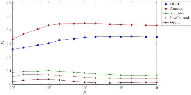
Figure 1: $F_{1}$ score as a function of the $N$ parameter with the aDCBM method.

• Fig. 1: $F_{1}$ score on SNAP datasets as a function of the $N$ parameter.

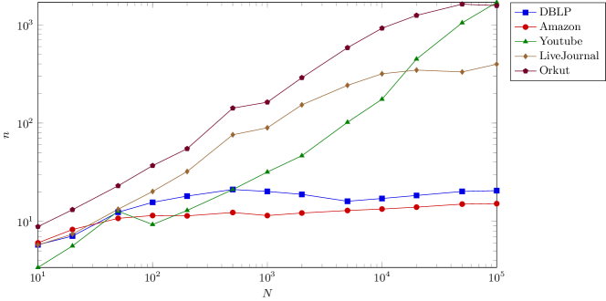
Figure 2: Mean community size as a function of the $N$ parameter with the aDCBM method.

• Fig. 2: Mean size of the recovered community as a function of $N$ parameter.

Table 3: Overview of the additional datasets.

Dataset	#node	#edge	#comm	$\overline{|c|}$
LFR (mu=0.1)	5000	25111	101	49.5
LFR (mu=0.2)	5000	25124	101	49.5
LFR (mu=0.3)	5000	25125	101	49.5
LFR (mu=0.4)	5000	25127	101	49.5
LFR (mu=0.5)	5000	25118	101	49.5
LFR (mu=0.6)	5000	25127	101	49.5
Amazon	334863	925872	151037	19.4
DBLP	317080	1049866	13477	53.4
Youtube	1134890	2987624	8385	13.5
LiveJournal	3997962	34681189	287512	22.3
Orkut	3072441	117185083	6288363	14.2
Amazon (top 5000)	334863	925872	5000	13.5
DBLP (top 5000)	317080	1049866	5000	22.4
Youtube (top 5000)	1134890	2987624	5000	14.6
LiveJournal (top 5000)	3997962	34681189	5000	27.8
Orkut (top 5000)	3072441	117185083	5000	215.7
Karate	34	78	2	17.0
Football	115	613	12	9.6
Pol.Blogs	1490	16715	2	745.0
Pol.Books	105	441	3	35.0
Flickr	35313	3017530	171	4336.1

Table 4: Mean size of the recovered communities.

	Global methods		Local methods
Dataset	gSBM	gDCBM	aSBM	aDCBM	aDCBM-1k	YL	LEMON	HK	PPR
LFR (mu=0.1)	48.9	49.0	20.5	45.7	44.2	9.4	50.2	159.0	1518.9
LFR (mu=0.2)	48.7	49.0	19.7	42.1	39.7	8.4	49.2	2264.6	2155.1
LFR (mu=0.3)	46.2	49.0	18.1	40.9	32.4	5.9	43.4	2410.0	2366.2
LFR (mu=0.4)	42.9	48.9	16.1	30.8	21.9	5.2	42.9	2398.3	2323.2
LFR (mu=0.5)	30.5	45.9	13.4	20.6	14.3	4.8	49.5	2412.0	2294.6
LFR (mu=0.6)	16.3	20.7	10.5	13.6	9.9	4.9	56.8	2412.8	2269.3
Amazon	23.9	33.6	11.1	16.3	11.5	6.4	41.9	88.8	20819.9
DBLP	27.6	39.8	11.2	21.3	20.2	6.0	46.2	55.0	24495.0
Youtube	1283.5	38.0	31.1	78.6	31.8	9.3	53.2	147.9	20955.5
LiveJournal	375.0	253.2	82.1	107.6	89.5	10.8	-	153.2	3428.7
Orkut	2089.9	1288.8	367.5	283.8	163.0	11.1	-	212.0	1634.0
Amazon (top 5000)	15.4	24.5	7.6	10.4	9.6	7.1	40.0	28.3	4828.6
DBLP (top 5000)	24.8	37.7	8.8	15.6	12.3	6.2	40.0	46.8	9506.8
Youtube (top 5000)	434.0	42.0	30.6	42.6	26.3	6.9	55.3	113.9	10867.7
LiveJournal (top 5000)	98.5	158.1	23.7	48.7	36.6	13.0	-	100.0	549.8
Orkut (top 5000)	973.5	1272.3	181.5	219.9	202.6	9.1	-	264.8	1607.4
Karate	2.8	2.0	4.6	6.2	15.3	8.8	15.0	16.7	17.1
Football	8.9	9.8	9.5	10.2	10.8	8.8	44.9	40.5	56.5
Pol.Blogs	100.7	18.0	45.1	20.3	97.9	7.2	68.2	492.7	1051.1
Pol.Books	10.7	21.1	12.3	9.1	25.2	6.7	43.3	49.3	53.4
Flickr	2796.9	608.5	1054.0	222.5	436.9	12.9	75.4	174.2	1158.1

Table 5: Mean precision of the recovered communities.

	Global methods		Local methods
Dataset	gSBM	gDCBM	aSBM	aDCBM	aDCBM-1k	YL	LEMON	HK	PPR
LFR (mu=0.1)	1.000	1.000	0.992	0.924	0.919	0.929	0.928	0.862	0.330
LFR (mu=0.2)	1.000	1.000	0.982	0.827	0.840	0.823	0.870	0.069	0.114
LFR (mu=0.3)	0.971	0.997	0.945	0.826	0.792	0.669	0.690	0.020	0.020
LFR (mu=0.4)	0.951	0.988	0.898	0.725	0.651	0.569	0.607	0.020	0.021
LFR (mu=0.5)	0.890	0.915	0.800	0.562	0.468	0.465	0.446	0.020	0.021
LFR (mu=0.6)	0.647	0.577	0.644	0.236	0.225	0.387	0.266	0.019	0.020
Amazon	0.256	0.175	0.385	0.376	0.409	0.422	0.157	0.166	0.088
DBLP	0.231	0.158	0.497	0.346	0.378	0.372	0.167	0.161	0.153
Youtube	0.023	0.035	0.082	0.058	0.066	0.086	0.047	0.024	0.037
LiveJournal	0.028	0.016	0.055	0.033	0.039	0.059	-	0.021	0.025
Orkut	0.005	0.004	0.012	0.008	0.010	0.032	-	0.020	0.012
Amazon (top 5000)	0.743	0.546	0.977	0.949	0.959	0.928	0.317	0.649	0.469
DBLP (top 5000)	0.343	0.233	0.740	0.548	0.594	0.544	0.229	0.274	0.260
Youtube (top 5000)	0.052	0.052	0.122	0.149	0.139	0.226	0.062	0.045	0.080
LiveJournal (top 5000)	0.405	0.275	0.696	0.641	0.623	0.592	-	0.479	0.400
Orkut (top 5000)	0.173	0.136	0.377	0.299	0.140	0.235	-	0.278	0.207
Karate	0.607	0.427	0.958	0.961	0.872	0.913	0.732	0.813	0.909
Football	0.825	0.818	0.755	0.686	0.768	0.828	0.204	0.371	0.154
Pol.Blogs	0.603	0.751	0.806	0.732	0.670	0.776	0.795	0.765	0.433
Pol.Books	0.625	0.610	0.641	0.624	0.616	0.699	0.596	0.587	0.586
Flickr	0.271	0.242	0.395	0.098	0.271	0.125	0.294	0.201	0.222

Table 6: Mean recall of the recovered communities.

	Global methods		Local methods
Dataset	gSBM	gDCBM	aSBM	aDCBM	aDCBM-1k	YL	LEMON	HK	PPR
LFR (mu=0.1)	0.999	1.000	0.453	0.909	0.892	0.232	0.940	0.995	1.000
LFR (mu=0.2)	0.997	1.000	0.425	0.811	0.792	0.218	0.865	1.000	1.000
LFR (mu=0.3)	0.957	0.997	0.380	0.794	0.713	0.114	0.561	1.000	1.000
LFR (mu=0.4)	0.907	0.993	0.322	0.647	0.510	0.077	0.503	1.000	1.000
LFR (mu=0.5)	0.706	0.914	0.248	0.438	0.297	0.052	0.439	1.000	0.999
LFR (mu=0.6)	0.362	0.366	0.168	0.130	0.071	0.041	0.330	0.971	0.964
Amazon	0.808	0.831	0.575	0.750	0.689	0.467	0.913	0.755	0.985
DBLP	0.543	0.593	0.421	0.495	0.416	0.223	0.701	0.483	0.853
Youtube	0.445	0.267	0.300	0.181	0.252	0.112	0.436	0.117	0.757
LiveJournal	0.346	0.345	0.286	0.172	0.260	0.081	-	0.193	0.661
Orkut	0.454	0.445	0.225	0.204	0.257	0.056	-	0.432	0.690
Amazon (top 5000)	0.967	0.972	0.792	0.901	0.883	0.763	0.943	0.977	0.997
DBLP (top 5000)	0.811	0.856	0.649	0.737	0.667	0.396	0.897	0.723	0.939
Youtube (top 5000)	0.669	0.605	0.421	0.483	0.420	0.364	0.714	0.272	0.826
LiveJournal (top 5000)	0.932	0.938	0.707	0.892	0.803	0.554	-	0.910	0.962
Orkut (top 5000)	0.663	0.683	0.396	0.463	0.175	0.095	-	0.530	0.711
Karate	0.101	0.060	0.241	0.317	0.721	0.446	0.641	0.794	0.913
Football	0.777	0.822	0.710	0.679	0.781	0.758	0.894	0.921	0.923
Pol.Blogs	0.129	0.020	0.055	0.023	0.069	0.008	0.084	0.593	0.707
Pol.Books	0.196	0.364	0.198	0.171	0.417	0.112	0.670	0.760	0.819
Flickr	0.259	0.089	0.127	0.049	0.046	0.012	0.022	0.042	0.125

Table 7: Mean runtime in seconds per community. Note that for the global methods a partition of the nodes is computed only once.

	Global methods		Local methods
Dataset	gSBM	gDCBM	aSBM	aDCBM	aDCBM-1k	YL	LEMON	HK	PPR
LFR (mu=0.1)	0.017	0.017	0.024	0.024	0.030	0.128	0.113	0.047	1.012
LFR (mu=0.2)	0.017	0.017	0.026	0.028	0.033	0.149	0.122	0.061	1.095
LFR (mu=0.3)	0.018	0.018	0.029	0.032	0.035	0.069	0.047	0.034	0.649
LFR (mu=0.4)	0.018	0.018	0.031	0.032	0.035	0.128	0.131	0.068	1.091
LFR (mu=0.5)	0.017	0.018	0.032	0.033	0.035	0.139	0.132	0.069	1.123
LFR (mu=0.6)	0.018	0.018	0.030	0.032	0.035	0.132	0.133	0.072	1.116
Amazon	0.036	0.035	0.022	0.023	0.029	4.418	1.564	0.031	2.803
DBLP	0.032	0.034	0.026	0.027	0.035	5.799	1.757	0.039	1.405
Youtube	0.059	0.055	0.854	1.138	0.200	18.975	4.959	0.074	0.514
LiveJournal	0.130	0.116	0.726	0.684	0.508	189.899	-	0.115	0.312
Orkut	0.095	0.095	7.551	4.923	3.487	1632.087	-	0.212	0.488
Amazon (top 5000)	0.034	0.032	0.020	0.018	0.027	2.629	1.559	0.022	1.643
DBLP (top 5000)	0.034	0.036	0.022	0.023	0.028	5.637	1.736	0.036	1.319
Youtube (top 5000)	0.056	0.056	0.707	0.398	0.146	18.295	4.855	0.078	0.520
LiveJournal (top 5000)	0.124	0.118	0.111	0.095	0.095	101.696	-	0.101	0.446
Orkut (top 5000)	0.101	0.088	1.960	1.774	2.144	1542.724	-	0.228	0.602
Karate	0.016	0.016	0.017	0.015	0.019	0.009	0.008	0.007	0.017
Football	0.016	0.016	0.017	0.016	0.020	0.019	0.012	0.006	0.046
Pol.Blogs	0.016	0.016	0.044	0.074	0.069	0.055	0.038	0.015	0.365
Pol.Books	0.016	0.016	0.018	0.016	0.021	0.011	0.008	0.006	0.040
Flickr	0.020	0.019	3.701	4.015	2.017	25.639	11.929	0.045	0.133

References

- Kloumann and Kleinberg (2014) I. M. Kloumann and J. M. Kleinberg, in Proceedings of the 20th ACM SIGKDD International Conference on Knowledge Discovery and Data Mining, KDD ’14 (ACM, New York, NY, USA, 2014) pp. 1366–1375.
- Andersen et al. (2006) R. Andersen, F. Chung, and K. Lang, in Foundations of Computer Science, 2006. FOCS’06. 47th Annual IEEE Symposium on (IEEE, 2006) pp. 475–486.
- Yang and Leskovec (2012) J. Yang and J. Leskovec, in Proceedings of the ACM SIGKDD Workshop on Mining Data Semantics, MDS ’12 (ACM, 2012) pp. 3:1–3:8.
- Li et al. (2015) Y. Li, K. He, D. Bindel, and J. E. Hopcroft, in Proceedings of the 24th International Conference on World Wide Web (International World Wide Web Conferences Steering Committee, 2015) pp. 658–668.
- Fortunato (2010) S. Fortunato, Physics Reports 486, 75 (2010).
- Shi and Malik (2000) J. Shi and J. Malik (IEEE Computer Society, Washington, DC, USA, 2000) pp. 888–905.
- Kloster and Gleich (2014) K. Kloster and D. F. Gleich, in Proceedings of the 20th ACM SIGKDD International Conference on Knowledge Discovery and Data Mining, KDD ’14 (ACM, New York, NY, USA, 2014) pp. 1386–1395.
- Xie et al. (2013) J. Xie, S. Kelley, and B. K. Szymanski, ACM Comput. Surv. 45, 43:1 (2013).
- Paul W. Holland (1983) S. L. Paul W. Holland, Kathryn Blackmond Laksey, Social Networks 5, 109 (1983).
- Carolyn J. Anderson (1992) K. F. Carolyn J. Anderson, Stanley Wasserman, Social Networks 14, 137 (1992).
- Karrer and Newman (2011) B. Karrer and M. E. J. Newman, Phys. Rev. E 83, 016107 (2011).
- Yan et al. (2014) X. Yan, C. Shalizi, J. E. Jensen, F. Krzakala, C. Moore, L. Zdeborová, P. Zhang, and Y. Zhu, Journal of Statistical Mechanics: Theory and Experiment 2014, P05007 (2014).
- Kemp et al. (2006) C. Kemp, J. B. Tenenbaum, T. L. Griffiths, T. Yamada, and N. Ueda, in Proceedings of the 21st National Conference on Artificial Intelligence - Volume 1, AAAI’06 (AAAI Press, 2006) pp. 381–388.
- Newman and Leicht (2007) M. E. J. Newman and E. A. Leicht, Proceedings of the National Academy of Sciences 104, 9564 (2007), http://www.pnas.org/content/104/23/9564.full.pdf .
- Psorakis et al. (2011) I. Psorakis, S. Roberts, M. Ebden, and B. Sheldon, Physical Review E 83, 066114+ (2011).
- Ball et al. (2011) B. Ball, B. Karrer, and M. E. J. Newman, Physical Review E 84, 036103 (2011).
- Zhang et al. (2007) H. Zhang, C. L. Giles, H. C. Foley, and J. Yen, in Proceedings of the 22Nd National Conference on Artificial Intelligence - Volume 1, AAAI’07 (AAAI Press, 2007) pp. 663–668.
- Blundell and Teh (2013) C. Blundell and Y. W. Teh, in Advances in Neural Information Processing Systems (2013).
- Hofman and Wiggins (2008) J. M. Hofman and C. H. Wiggins, Phys Rev Lett 100, 258701 (2008), 18643711[pmid].
- Decelle et al. (2011) A. Decelle, F. Krzakala, C. Moore, and L. Zdeborová, Phys. Rev. E 84, 066106 (2011).
- Zhang et al. (2016) P. Zhang, C. Moore, and M. E. J. Newman, Phys. Rev. E 93, 012303 (2016).
- Palla et al. (2005) G. Palla, I. Derenyi, I. Farkas, and T. Vicsek, Nature 435, 814 (2005).
- Fortunato and Barthélemy (2007) S. Fortunato and M. Barthélemy, Proceedings of the National Academy of Sciences of the United States of America 104, 36 (2007).
- Reichardt and Bornholdt (2004) J. Reichardt and S. Bornholdt, Physical Review Letters 93, 218701 (2004).
- Blondel et al. (2008) V. D. Blondel, J.-L. Guillaume, R. Lambiotte, and E. Lefebvre, Journal of Statistical Mechanics: Theory and Experiment 2008, P10008 (2008), arXiv:0803.0476 .
- Lancichinetti et al. (2008) A. Lancichinetti, S. Fortunato, and F. Radicchi, Physical Review E 78, 046110 (2008).
- Leskovec and Krevl (2014) J. Leskovec and A. Krevl, “SNAP Datasets: Stanford large network dataset collection,” http://snap.stanford.edu/data (2014).
- Wang et al. (2012) X. Wang, L. Tang, H. Liu, and L. Wang, Knowledge and Information Systems (KAIS) (2012), 10.1007/s10115-012-0555-0.
- Zachary (1977) W. W. Zachary, Journal of Anthropological Research 33, 452 (1977).
- Girvan and Newman (2002) M. Girvan and M. E. J. Newman, Proceedings of the National Academy of Sciences of the United States of America 99, 7821 (2002).
- Krebs (2004) V. Krebs, “New political patterns,” Editorial (2004).
- Adamic and Glance (2005) L. Adamic and N. Glance, in LinkKDD ’05: Proceedings of the 3rd international workshop on Link discovery (2005) pp. 36–43.
- McDaid and Hurley (2010) A. McDaid and N. Hurley, in Proceedings of the 2010 International Conference on Advances in Social Networks Analysis and Mining, ASONAM ’10 (IEEE Computer Society, Washington, DC, USA, 2010) pp. 112–119.