Large proton cumulants from the superposition of ordinary multiplicity distributions

Abstract

We construct a multiplicity distribution characterized by large factorial cumulants (integrated correlation functions) from a simple combination of two ordinary multiplicity distributions characterized by small factorial cumulants. We find that such a model, which could be interpreted as representing two event classes, reproduces the preliminary data for the proton cumulants measured by the STAR collaboration at $7.7$ GeV very well. This model then predicts very large values for the fifth and sixth order factorial cumulants, which can be tested in experiment.

I Introduction

The study of fluctuations and correlations of conserved charges has become the focus of attention in the search of the QCD phase transition and its conjectured critical point Stephanov (2004, 2009); Skokov et al. (2011); Stephanov (2011); Luo et al. (2012); Luo and Xu (2017); Herold et al. (2016); Zhou et al. (2012); Wang and Yang (2012); Karsch and Redlich (2011); Schaefer and Wagner (2012); Chen et al. (2011); Fu et al. (2010); Cheng et al. (2009); Jeon and Koch (2000); Gazdzicki et al. (2004); Gorenstein et al. (2004); Gazdzicki et al. (2004); Koch et al. (2005); Alt et al. (2008, 2009). While at vanishing chemical potential lattice QCD calculations have established that the transition occurs as an analytic crossover Aoki et al. (2006); Borsanyi et al. (2010); Bazavov et al. (2012), no real constraints on the phase transition at large chemical potential are currently possible. Therefore one mainly relies on experimental studies to identify the order of the QCD phase transition. If indeed a first order phase transition occurs at large baryon chemical potentials and intermediate temperatures, also an associated endpoint must exist at which the transition becomes second order. It is well known that first and second order phase transitions give rise to many interesting phenomena, especially related to fluctuations and long range correlations Jeon and Koch (2000); Koch (2010). In macroscopic systems that slowly approach a second order phase transition the correlation length diverges and similarly systems that approach a first order phase transition will undergo nucleation, leading to droplet formation, or spinodal decomposition Chomaz et al. (2004); Randrup (2004); Sasaki et al. (2007); Randrup (2009); Nahrgang et al. (2011); Mishustin (1999); Steinheimer and Randrup (2012). One observable of particular interest are higher order cumulants of the proton number distribution. It has been shown Stephanov (2009) that, close to the critical point, higher orders of the cumulants diverge with ever increasing powers of the correlations length.

The goal of several experimental programs at RHIC, SPS, NICA, J-PARC and GSI/FAIR facilities is to identify observables which would show the increase of particle correlations and fluctuations due to a phase transition. To do so, heavy nuclei are brought to collision at relativistic energies. The system created in such collisions may have densities several times that of normal nuclear saturation density and temperatures of more than 200 MeV Damjanovic et al. (2009); Specht (2010), a finding supported by microscopic transport simulations as well as fluid dynamical simulations (see e.g. Rapp and van Hees (2016); Endres et al. (2016); Steinheimer et al. (2010)) at the energies discussed.

In addition, by varying the beam energy of the collision one is able to change the density and temperature of the created system, which allows to ’scan’ the phase diagram of QCD and hopefully locate the onset of phase transition signals.

The systems created in these heavy ion collisions are very small (a few fm in size) rapidly expanding (the expansion velocity is close to the speed of light) and short lived (the system decouples after 10-20 fm/c). These features affect possible signals of a phase transition. For example, there may not be sufficient time for the correlation length to grow significantly near the critical point Berdnikov and Rajagopal (2000) or for nucleation, which is also a comparatively slow process, to occur. On the other hand phenomena like spinodal decomposition, i.e., the rapid phase separation due to (mechanical) instabilities at the phase transition are much faster due to the exponential growth of fluctuations in the mechanically unstable region, and thus can occur resulting in an increase of density fluctuations Steinheimer and Randrup (2012); Herold et al. (2013). Further complications arise from the fact that the number of charge, strangeness or baryon number carrying particles is relatively small, especially for the baryon number. As a consequence, effects of the global conservation of the various conserved charges cannot be neglected Begun et al. (2004); Nahrgang et al. (2012); Bzdak et al. (2013). In addition, as the system rapidly drops out of equilibrium, other effects like resonance decays, thermal smearing may blur the signal. Additionally, experimental acceptance and efficiency corrections need to be taken into account Bzdak and Koch (2012); Bzdak et al. (2016); Kitazawa (2016); He and Luo (2018); Fecková et al. (2015); Begun et al. (2004); Bzdak et al. (2013); Gorenstein et al. (2009); Gorenstein and Gazdzicki (2011); Sangaline (2015); Tarnowsky and Westfall (2013); Xu (2014); Adamczyk et al. (2014a, b).

Published data on the net-proton number fluctuations, which, with reasonable model assumptions, can be related to the net-baryon fluctuations Kitazawa and Asakawa (2012a, b), only exist from the STAR collaboration Adamczyk et al. (2014b); Aggarwal et al. (2010) and for a limited acceptance. The published data ($|y|<0.5$ and $0.4<p_{t}<0.8$ GeV) are consistent with uncorrelated proton production and the trivial correlations from global baryon conservation Bzdak et al. (2013). On the other hand preliminary data from the STAR collaboration with a larger acceptance ($0.4<p_{t}<2$ GeV) Luo (2015, 2016) show a significant deviation from uncorrelated proton emission, i.e., following Poisson statistics, for collision energies $\sqrt{s_{NN}}\leq 11{\rm\,GeV}$. The preliminary data consistently show an increase of the fourth order cumulant and a decrease of the third order cumulant with respect to uncorrelated production, in particular at the lowest beam energies of $\sqrt{s_{NN}}=7.7{\rm\,GeV}$ and $\sqrt{s_{NN}}=11{\rm\,GeV}$. Presently, higher order net-proton cumulants are also being studied in other experiments, such as HADES Lorenz (2017) and NA61 Davis et al. (2017); Gazdzicki (2018).

The experiments provide the measured cumulants of the net-proton number distributions and not the actual multi-particle correlation functions. However, the integrated n-particle correlation functions (factorial cumulants) can be extracted from the measured cumulants Bzdak et al. (2017a) and they indeed show an interesting beam energy dependence. In particular, the integrated four particle correlations at the lowest beam energy accessible to STAR, $\sqrt{s_{NN}}=7.7{\rm\,GeV}$ are very large, about three orders of magnitude larger than a basic Glauber model (incorporating the number of wounded nucleons Bialas et al. (1976) fluctuations) combined with baryon number conservation would predict Bzdak et al. (2017b). The challenge now is to unambiguously connect the measured correlations to physical effects from a critical point or first order phase transition.

In this paper we will investigate how one can construct a proton multiplicity distribution, consistent with the unexpectedly large, as compared to expectations from conventional models Bzdak et al. (2017b); He and Luo (2017), factorial cumulants extracted Bzdak et al. (2017a) from the recent preliminary STAR measurements at $\sqrt{s_{NN}}=7.7{\rm\,GeV}$. To this end we will focus on the case where the proton distribution function results from a superposition of two independent distributions, or sources of protons. In particular we want to explore if it is possible to construct such a superposition for the case where individual distributions are both characterized by small factorial cumulants. In principle there are two distinct ways to construct such a superposition of two sources/distribution: In the first scenario, one assumes that in each event the protons arise from both sources at the same time and thus the total proton number is simply the sum of the protons drawn from the two distributions. As we shall discuss in the paper, in this case the factorial cumulants of the combined distribution are of the same order of magnitude as those of the two individual distributions. In the second scenario, one assumes that the superposition of two independent distributions is such that in a given event the proton multiplicity is drawn exclusively, with a certain probability, from either one of the two distributions. This case corresponds to having two distinct event classes, and as we shall show, the factorial cumulants of the combined distribution can be very large even if the factorial cumulants of the individual distributions are small or even vanish as it would be the case if we were using Poissonians. It is this second scenario which we will concentrate on in this paper. In particular we will discuss the extracted Bzdak et al. (2017a) factorial cumulants from the STAR experiment in the context of such multiplicity distributions. Possible interpretations in terms of phase transition physics and ’non-physics’ background will be given. Furthermore we will propose further experimental studies which will help to better understand the origin of experimentally measured large correlations.

II Two events classes

Let us consider the situation where we have two different types (or classes) of events, denoted by (a) and (b). Let us denote the probability that an event belongs to class (a) by $(1-\alpha)$ and to class (b) by $\alpha$ with $\alpha\leq 1$. In this case the probability to find $N$ particles or protons is given by

$$P(N)=(1-\alpha)P_{(a)}(N)+\alpha P_{(b)}(N),$$ (1)

where $P_{(a)}(N)$ and $P_{(b)}(N)$ are multiplicity distributions governing the event classes (a) and (b) respectively. As we shall show, the combined distribution, Eq. (1), can exhibit very large factorial cumulants (integrated correlation functions) even if neither $P_{(a)}$ nor $P_{{(b)}}$ exhibit any correlations, as would be the case if they were Poissonian. Such a situation can arise for example if in a heavy ion experiment the centrality selection, for whatever reasons, mixes central events with very peripheral ones.

In order to calculate the factorial cumulants it is best to start with the generating function:

$$H(z) = \sum P(N)z^{N}$$ (2)

$$= (1-\alpha)H_{(a)}(z)+\alpha H_{(b)}(z).$$

where $H_{(a),(b)}$ is the generating function for $P_{(a),(b)}$. The factorial cumulant generating function is then given by

$$G(z) = \ln\left[H(z)\right]$$ (3)

$$= \ln\left[(1-\alpha)H_{(a)}(z)+\alpha H_{(b)}(z)\right]$$

$$= \ln\left[(1-\alpha)e^{\ln[H_{(a)}(z)]}+\alpha e^{\ln[H_{(b)}(z)]}\right]$$

$$= G_{(a)}(z)+\ln\left[1-\alpha+\alpha e^{G_{(b)}(z)-G_{(a)}(z)}\right],$$

where $G_{(a),(b)}(z)=\ln[H_{(a),(b)}(z)]$. The factorial cumulants read

$$C_{k}=\left.\frac{d^{k}}{dz^{k}}G(z)\right|_{z=1},$$ (4)

and analogously for $C_{k}^{(a)}=\frac{d^{k}}{dz^{k}}G_{(a)}(z)|_{z=1}$ and $C_{k}^{(b)}=\frac{d^{k}}{dz^{k}}G_{(b)}(z)|_{z=1}$.

Given the distribution Eq. (1), the mean number of protons is

$$\left\langle N\right\rangle=(1-\alpha)\left\langle N_{(a)}\right\rangle+\alpha\left\langle N_{(b)}\right\rangle,$$ (5)

with $\left\langle N_{(a),(b)}\right\rangle=\sum_{N}NP_{(a),(b)}(N)$ is the average particle number for distributions $P_{(a)}(N)$ and $P_{(b)}(N)$, respectively. To simplify the notation we further introduce

$$\mkern 1.5mu\overline{\mkern-1.5muN\mkern-1.5mu}\mkern 1.5mu = \left\langle N_{(a)}\right\rangle-\left\langle N_{(b)}\right\rangle,$$

$$\mkern 1.5mu\overline{\mkern-1.5muC\mkern-1.5mu}\mkern 1.5mu_{n} = C_{n}^{(a)}-C_{n}^{(b)},$$ (6)

and performing straightforward calculations we obtain,

$$C_{2}=C_{2}^{(a)} - \alpha\left\{\mkern 1.5mu\overline{\mkern-1.5muC\mkern-1.5mu}\mkern 1.5mu_{2}-(1-\alpha)\mkern 1.5mu\overline{\mkern-1.5muN\mkern-1.5mu}\mkern 1.5mu^{2}\right\},$$

$$C_{3}=C_{3}^{(a)} - \alpha\left\{\mkern 1.5mu\overline{\mkern-1.5muC\mkern-1.5mu}\mkern 1.5mu_{3}+(1-\alpha)\left[(1-2\alpha)\mkern 1.5mu\overline{\mkern-1.5muN\mkern-1.5mu}\mkern 1.5mu^{3}-3\mkern 1.5mu\overline{\mkern-1.5muN\mkern-1.5mu}\mkern 1.5mu\mkern 1.5mu\overline{\mkern-1.5muC\mkern-1.5mu}\mkern 1.5mu_{2}\right]\right\},$$

$$C_{4}=C_{4}^{(a)} - \alpha\left\{\mkern 1.5mu\overline{\mkern-1.5muC\mkern-1.5mu}\mkern 1.5mu_{4}-(1-\alpha)\left[\left(1-6\alpha+6\alpha^{2}\right)\mkern 1.5mu\overline{\mkern-1.5muN\mkern-1.5mu}\mkern 1.5mu^{4}\right.\right.$$ (7)

$$- \left.\left.6(1-2\alpha)\mkern 1.5mu\overline{\mkern-1.5muN\mkern-1.5mu}\mkern 1.5mu^{2}\mkern 1.5mu\overline{\mkern-1.5muC\mkern-1.5mu}\mkern 1.5mu_{2}+4\mkern 1.5mu\overline{\mkern-1.5muN\mkern-1.5mu}\mkern 1.5mu\mkern 1.5mu\overline{\mkern-1.5muC\mkern-1.5mu}\mkern 1.5mu_{3}+3(\mkern 1.5mu\overline{\mkern-1.5muC\mkern-1.5mu}\mkern 1.5mu_{2})^{2}\right]\right\}.$$

So far the results are general and apply for an arbitrary choice of distributions $P_{(a)}$ and $P_{(b)}$.

Our goal here is to obtain large factorial cumulants $C_{n}$ from ordinary multiplicity distributions characterized by small factorial cumulants, namely $C_{n}^{(a)}\ll C_{n}$ and $C_{n}^{(b)}\ll C_{n}$. This is motivated by a surprisingly large three- and four-proton factorial cumulants, $C_{3}$ and $C_{4}$, measured in central Au+Au collisions at $\sqrt{s_{NN}}=7.7$ GeV, which are much larger than simple expectations from baryon conservation or $N_{\rm part}$ fluctuation. The ultimate case where this holds is when the two classes are governed by Poisson distributions, where $C_{n}^{(a)}=C_{n}^{(b)}=0$. In this case the factorial cumulants reduce to

$$C_{2} = \alpha(1-\alpha)\mkern 1.5mu\overline{\mkern-1.5muN\mkern-1.5mu}\mkern 1.5mu^{2}\approx\alpha\mkern 1.5mu\overline{\mkern-1.5muN\mkern-1.5mu}\mkern 1.5mu^{2},$$

$$C_{3} = -\alpha(1-\alpha)(1-2\alpha)\mkern 1.5mu\overline{\mkern-1.5muN\mkern-1.5mu}\mkern 1.5mu^{3}\approx-\alpha\mkern 1.5mu\overline{\mkern-1.5muN\mkern-1.5mu}\mkern 1.5mu^{3},$$

$$C_{4} = \alpha(1-\alpha)(1-6\alpha+6\alpha^{2})\mkern 1.5mu\overline{\mkern-1.5muN\mkern-1.5mu}\mkern 1.5mu^{4}\approx\alpha\mkern 1.5mu\overline{\mkern-1.5muN\mkern-1.5mu}\mkern 1.5mu^{4},$$ (8)

where in the last step we assumed $\alpha\ll 1$. In general, for small $\alpha$ we have ($n>1$)

$$C_{n}\approx(-1)^{n}\alpha\mkern 1.5mu\overline{\mkern-1.5muN\mkern-1.5mu}\mkern 1.5mu^{n},\quad\alpha\ll 1,\quad n>1$$ (9)

and the higher order factorial cumulants can assume very large values even for small values of $\alpha$.

In general, if the measured $C_{n}\gg C_{n}^{(a)}$ and $C_{n}\gg C_{n}^{(b)}$, we obtain Eqs. (8) and (9). In this case, $C_{n}$ is independent of the details of $P_{(a)}(N)$ and $P_{(b)}(N)$, and the signal is driven almost exclusively by the superposition between the two distributions. This results in the relation between factorial cumulants of adjacent order

$$\frac{C_{n+1}}{C_{n}}\approx-\mkern 1.5mu\overline{\mkern-1.5muN\mkern-1.5mu}\mkern 1.5mu,$$ (10)

for $\alpha\ll 1$ with the first correction being $\mathcal{O}(\alpha\mkern 1.5mu\overline{\mkern-1.5muN\mkern-1.5mu}\mkern 1.5mu)$. Also in this limit, the above ratio does not depend on $\alpha$. At $7.7$ GeV, $C_{4}/C_{3}\sim-17$, see Ref. Bzdak et al. (2017a), (with admittedly large error bars). Our approach clearly predicts the ratio of higher order cumulants, as well as the fact that their signs are alternating, see Eq. (9), which can be tested by future experimental data on $C_{5}/C_{4}$ and $C_{6}/C_{5}$. To summarize, if indeed the large factorial cumulants observed at $7.7$ GeV originate from the superposition of two event classes with $\alpha\ll 1$, we expect

$$\frac{C_{6}}{C_{5}}\approx\frac{C_{5}}{C_{4}}\approx\frac{C_{4}}{C_{3}}=-17\pm 6,$$ (11)

where the uncertainty is based on $C_{4}=170\pm 45$ and $C_{3}=-10\pm 2.5$ Bzdak et al. (2017a).

In Bzdak et al. (2017a); Bzdak and Koch (2017) it was shown that the integrated correlation functions (factorial cumulants) obtained from the STAR measurements are consistent with rapidity and transverse momentum independent normalized multi-particle correlation functions. In other words, the STAR data are consistent with a very large correlation length in rapidity and transverse momentum. This in turn implies that the factorial cumulants scale with the mean proton number like $C_{n}\sim\langle N\rangle^{n}$. As seen from Eqs. (8) and (9), valid if $C_{n}\gg C_{n}^{(a)}$ and $C_{n}\gg C_{n}^{(b)}$, this is naturally explained in our superposition model. Indeed, if we were really dealing with two event classes, the relative weight of the two distributions, $\alpha$, would be independent of the size of the rapidity window, whereas the mean number of particles from event types (a) and (b) would roughly scale with the rapidity window $\langle N_{(a)}\rangle\sim\Delta Y$ and $\langle N_{(b)}\rangle\sim\Delta Y$. Consequently $\langle N\rangle\sim\Delta Y$ and $\mkern 1.5mu\overline{\mkern-1.5muN\mkern-1.5mu}\mkern 1.5mu\sim\Delta Y$. As a result, $\mkern 1.5mu\overline{\mkern-1.5muN\mkern-1.5mu}\mkern 1.5mu\sim\Delta Y\sim\langle N\rangle$. Of course, this observation constitutes no proof for the existence of two event classes in the STAR data, as there may very well be other distributions with a similar scaling, but it certainly is a nice consistency check.

We note that our model is not well suited for multiplicity distributions characterized by small $C_{n}$. In this case the details of $C_{n}^{(a)}$ and $C_{n}^{(b)}$ are crucial and we loose any predictive power. However, if $C_{n}$ is small, there is most likely no need to introduce two event classes and the signal may very well be explained by an ordinary background. This is, e.g., the case for $\sqrt{s_{NN}}=19$ GeV collisions, where the measured $C_{3}$ and $C_{4}$ are close to zero and, in fact, are consistent (withing larger error bars) with simple baryon conservation with possible contribution from $N_{\rm part}$ fluctuation.

The main finding of this Section is that our model of two event classes indeed leads to large values for the higher order factorial cumulants and that we predict a straightforward relation between them, Eqs. (10) and (11), which can be tested in experiment. Next let us turn to a somewhat more refined analysis of the STAR data at $\sqrt{s_{NN}}=7.7{\rm\,GeV}$.

II.1 Data analysis

From the analysis Bzdak et al. (2017a) of the preliminary STAR data Luo (2015) we know that for central collisions at $\sqrt{s_{NN}}=7.7{\rm\,GeV}$ the factorial cumulants of the proton multiplicity distribution up to fourth order are

STAR: $$\langle N\rangle\approx 40,\,C_{2}\approx-2,\,C_{3}\approx-10,\,C_{4}\approx 170.$$

and, as already pointed out, $C_{3}$ and $C_{4}$ are much larger than expectations from an ordinary background, such as baryon conservation and $N_{\rm part}$ fluctuation Bzdak et al. (2017b).

Thus we are in the situation discussed in the previous section, where the superposition of two ordinary multiplicity distributions, Eq. (1), can easily generate large factorial cumulants which are independent on the specific choice for $P_{(a)}(N)$ and $P_{(b)}(N)$, provided $C^{(a)}_{n}$ and $C^{(b)}_{n}$ are much smaller then the measured $C_{n}$, see Eqs. (8) and (9). The simplest choice is to take Poisson distributions for both $P_{(a)}$ and $P_{(b)}$. The next refinement is to use a binomial distribution for $P_{(a)}$ in order to capture the effect of baryon number conservation Bzdak et al. (2017b). This actually results in $C_{2}<0$, as seen in the data.

Consequently, we take $P_{a}(N)$ as binomial,

$$P_{a}(N)=\frac{B!}{N!(B-N)!}p^{N}(1-p)^{B-N},$$ (12)

with $B=350$, which properly captures baryon number conservation, and $P_{b}(N)$ as Poisson. In this case the relevant factorial cumulants are given by

$$C_{2}^{(a)} = -p^{2}B,\quad C_{3}^{(a)}=2p^{3}B,\quad C_{4}^{(a)}=-6p^{4}B,$$

$$C_{5}^{(a)} = 24p^{5}B,\quad C_{6}^{(a)}=-120p^{6}B,$$ (13)

with $\langle N_{(a)}\rangle=pB$. Obviously $C^{(b)}_{n}=0$ and $\mkern 1.5mu\overline{\mkern-1.5muC\mkern-1.5mu}\mkern 1.5mu_{n}=C^{(a)}_{n}$.

Using Eqs. (7) we fit the mean number of protons as well as the third and the fourth order factorial cumulants resulting in

$$\alpha\approx 0.0033,\quad\mkern 1.5mu\overline{\mkern-1.5muN\mkern-1.5mu}\mkern 1.5mu\approx 14.7,\quad p\approx 0.114,$$ (14)

which also gives $\langle N_{(a)}\rangle\approx 40$ and $\langle N_{(b)}\rangle\approx 25.3$. We note that indeed $\alpha\ll 1$ as assumed in Eqs. (9), (10) and (11).

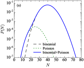
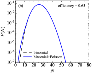
Figure 1: The multiplicity distribution $P(N)$ at $\sqrt{s_{NN}}=7.7{\rm\,GeV}$ in the two component model given by Eq. (1) constructed with (a) efficiency unfolded values for $\langle N\rangle$, $C_{3}$ and $C_{4}$ and (b) with imposed efficiency of $0.65$.

Given the fit, we can also predict the factorial cumulants, $C_{2}$, $C_{5}$, $C_{6}$ and we obtain:

$$C_{2} \approx-3.85,$$

$$C_{5} \approx-2645,$$

$$C_{6} \approx 40900,$$ (15)

which corresponds to the following values for the cumulant ratios

$$K_{5}/K_{2} \approx-34,$$

$$K_{6}/K_{2} \approx 312.$$ (16)

It is worth pointing out that $C_{6}/C_{5}\approx C_{5}/C_{4}\approx C_{4}/C_{3}$ in agreement with the discussion presented in the previous Section. We note that the resulting $C_{2}\approx-3.85$ is slightly more negative than the data. However, as shown, e.g., in Bzdak et al. (2017b), the second order factorial cumulant receives a sizable positive contribution from participant fluctuations $\Delta C_{2}\simeq 2-3$ whereas the correction to $C_{3}$ and $C_{4}$ are small. In any case correcting data for the fluctuations of $N_{\rm part}$ should be done very carefully to avoid model dependencies. In view of the sizable errors in the preliminary STAR data we consider the present fit as satisfactory.

The resulting probability distribution for the proton number, $P(N)$, Eq. (1), is shown in the left panel of Fig. 1. Even though the component centered at $N\sim 25$ has a very small probability $\alpha\sim 0.3\%$ it gives rise to a shoulder at low $N$ which should be visible in the multiplicity distribution. However, this would require an unfolding of the measured distribution Bzdak et al. (2016) in order to remove the effect of a finite detection efficiency. Assuming a binomial model for the efficiency with a constant detection probability of $\epsilon=0.65$, which roughly corresponds to that of the STAR measurement, the observed multiplicity distribution of the two component model is shown in the right panel of Fig. 1. In this case the small component $\sim\alpha$ is barely visible. This observation is consistent with the fact that the efficiency uncorrected cumulants measured by STAR are more or less consistent with a Poisson (or binomial to be more precise) expectation.

Another complication arises from the fact that the proton distribution functions are only measured in rather broad centrality bins. Directly correcting the distribution functions for this centrality bin-width effect is not straight forward. One should also note, that we only considered the most central data, as only here one observes significantly large correlations, i.e., $C_{n}^{(a)}\ll C_{n}$. For more peripheral centrality bins the situation is less clear, as the correlations, $C_{n}$, become smaller, which does not allow for a clear distinction between a single ordinary distribution and the superposition of two distributions.

For the next phase of the RHIC beam energy scan, it is expected that STAR may be able to increase its rapidity coverage. If it could be doubled, and the observed scaling $C_{n}\sim\left\langle N\right\rangle^{n}$ persists, the resulting probability distribution would look like Fig. 2. In this case, even with an efficiency of $\epsilon\simeq 0.65$ the two components should be visible in the efficiency uncorrected data.

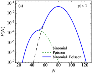
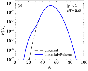
Figure 2: $P(N)$ for 7 GeV and twice the rapidity coverage as the present preliminary STAR data. See text for details.

III Discussion and conclusions

To understand the relevance of the previous results several comments are in order:

1. The factorial cumulants (integrated genuine correlation functions) based on the present STAR data in central $\sqrt{s_{NN}}=7.7$ GeV collisions are consistent with the assumption of two distinct event classes. This model not only reproduces the factorial cumulants but also naturally explains the long correlation length observed in the STAR data.

2. Provided that the measured factorial cumulants $C_{n}$ are much larger than expectations from an ordinary background (baryon conservation etc.) we predict that the factorial cumulants satisfy a simple relation given in Eq. (10), that is, $C_{n+1}/C_{n}$ does not depend on $n$. This can be tested in experiment by comparing $C_{4}/C_{3}$ with $C_{5}/C_{4}$ and $C_{6}/C_{5}$.

3. If indeed two event classes are at play, we predict that the 5th and 6th order factorial cumulants are very large. In addition, with the increasing acceptance of the STAR detector to be expected in the next phase of the RHIC beam energy scan, the third and forth order factorial cumulants should increase leading to a probability distribution which should exhibit a clear second event class which might even be visible without unfolding the data.

4. In the STAR experiment events are selected in centrality classes by the number of charged particles (other than protons and anti-protons) within the STAR acceptance Adamczyk et al. (2014b); Luo (2015). Therefore, in order to have two distinct event classes one of two things need to happen: Either there is a mechanism which removes protons from a central event which has many charged particles. Or, for some reason there are peripheral events, where naturally only few protons are stopped and brought to mid rapidity, but at the same time lots of charged particles (i.e. pions) are produced and the event is classified as a central one. The latter situation is hard to fathom (as far as originating from a physical effect). However, one could imagine that the observed lack of protons in some central events is compensated by an abundance of deuterons or other light nuclei. If true, this would result in a significant anti-correlation between the proton and deuteron number.

5. The present STAR dataset for $\sqrt{s_{NN}}=7.7$ GeV contains 3 million events so that the most central 5% correspond to 150k events Adamczyk et al. (2014b). Given $\alpha\approx 0.0033$ there are roughly 500 events for $N<20$ and it maybe worthwhile to inspect these events individually to see if there are some systematic deviations or common experimental issues. Indeed, in a recent paper He and Luo (2018) the possibility that a certain subset of events could have different/fluctuating efficiency has been discussed, and it was shown that such a scenario would effectively result in two or more event classes.

   

   

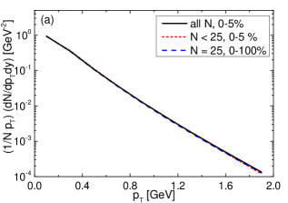
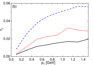
   Figure 3: (a): Transverse momentum distributions of charged pions from the UrQMD transport model. (b) Elliptic flow of charged pions as a function of the transverse momentum from UrQMD simulations. In both plots three different event selections are compared. The black solid lines correspond to all most central (0-5$\%$) events, while the red short dashed lines depict only most central events with a small proton number ($N<25$). The blue dashed lines correspond to the reference events with exactly 25 protons, but selected from all centralities.

   

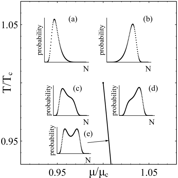
   Figure 4: Probability distribution at various points close to the co-existence line for the van der Waals model for system at fixed volume: $(T/T_{c},\mu/\mu_{c})=$ (1.02, 0.99) (a), (1.02, 1.004) (b), (0.98, 1.0015) (c), (0.98, 1.004) (d), (0.95, 1.0062) (e). The model and parameters are described in the Appendix B.

6. The natural way to explore the possible presence of distinct event classes in the STAR data, is to select events with a small number of protons (in central events) to enrich the contribution of the small event class. Then one can investigate whether these events exhibit certain characteristics, which distinguishes them from all other events in that centrality class. Such an event characteristic could be any other observable such as, e.g., the mean transverse momentum, the elliptic flow $v_{2}$, HBT radii etc. Of course some observables may change with the proton number even if there are no separate event classes. To illustrate this and to set some kind of baseline for the case where we do not have distinct event classes, we show the charged pion transverse momentum distributions and elliptic flow from UrQMD simulations, as function of the transverse momentum in Figs. 3 (a) and (b). To produce these results 30 million minimum bias UrQMD events of Au+Au collisions at a beam energy of $\sqrt{s_{NN}}=7.7{\rm\,GeV}$ were generated. Then the 0-5$\%$ most central events where selected as the most central bin, and are plotted as black-full lines. Here we used the same event selection as used in the STAR analysis, namely the centrality was determined by the number of charged particles (except protons and anti-protons) in $|y|\leq 1$. The number of protons is also determined in the STAR acceptance, $|y|\leq 0.5$ and $0.4\leq p_{T}\leq 2.0$ GeV, which gives a mean net-proton number of $\left\langle N\right\rangle\approx 42$. From these 0-5$\%$ most central events we then selected the 0.3$\%$ events with the smallest number of net protons ($N<25$), i.e., the left tail of the net proton multiplicity distribution, which is shown as red-dotted lines. This effect stems only from the fact that even different events in a given centrality class will have varying $v_{2}$. As a comparison we also selected, from all minimum bias events, only the events with a net proton number of $N=25$, shown as blue-dashed lines. Interestingly the resulting transverse momentum distributions seem almost independent of the event selection (the actual difference between the curves is less than 5%)
   On the other hand, the elliptic flow, $v_{2}$, depends rather strongly on the event selection. The most central events exhibit the smallest and the more peripheral events (blue line) have the largest elliptic flow. However, the central events with the smallest number of protons also show an increased $v_{2}$ compared to all central events. This is understandable, as the left tail of the proton distribution for the most central events contains a larger number of ’peripheral’ events, i.e., events with a larger impact parameter and therefore larger initial anisotropy.
   We can therefore conclude that the elliptic flow is a good criterion to select events based on their initial anisotropy. As a consequence, if STAR finds that the elliptic flow in the left tail (small number of protons) of the most central events has an elliptic flow which is as large as the elliptic flow in peripheral events with the same proton number, the additional events are likely due to misidentified peripheral events. On the other hand if STAR finds that the events in the low proton number tail have a $v_{2}$ equal to or smaller than the average of all central events, interesting physics may be at play. This would also be the case if one would find a significant deviation in the transverse momentum spectra for the evens in the lower tail of the most central events.

7. It is noteworthy that two event classes distribution looks very similar to that of a system close to a first order phase transition in a finite system. To illustrate this, we have used the van der Waals model in a finite volume to calculate the multiplicity distributions for various points near the co-existence line for a system of fixed volume (details are in the Appendix B). This is shown in Fig. 4. The multiplicity distribution extracted from the STAR cumulants, Fig. 1, looks qualitatively similar to the distribution to the right of the phase-coexistence line in Fig. 4. In this case the “bump” at small $N$ corresponds to events where the system would be in the “dilute” phase whereas the large maximum at large $N$ corresponds to the events where the system is in the “dense” phase, which dominates the distribution.

8. Naturally, the knowledge of only four factorial cumulants, $C_{1},\ldots,C_{4}$ does not uniquely determine the multiplicity distribution. And indeed applying the methods of Audenaert (2008) based on the Poisson-Charlier expansion (see Appendix C for some details) one can generate a different distribution which also reproduces the factorial cumulants of the preliminary STAR data. We verified that this distribution shows a much smaller shoulder on the left as the two event classes model used here. While the first four cumulants are the same for the two distributions by construction, the prediction for the fifth and sixth differ dramatically, as this distribution results in $C_{5}=-200$ and $C_{6}=4220$, which are about an order of magnitude smaller than that of the two event classes model. If, on the other hand, we enforce the $C_{5}$ and $C_{6}$ to be of the same magnitude as the two classes model, the resulting probability distribution from the Poisson-Charlier method develops a shoulder at low $N$ similar to the one of the two classes model. In other words, if the magnitude of the predicted values of $C_{5}$ and $C_{6}$ in Eq. (15) are confirmed by experiment, the presence of a shoulder at low $N$ is very likely, thus favoring the two event classes hypothesis.

9. Instead of two distinct event classes one could have the situation, where we have two mechanisms contributing at the same time to each event. In this case the multiplicity distribution is given by

   $$P(N)=\sum_{N_{(a)},N_{(b)}}P_{(a)}(N_{(a)})P_{(b)}(N_{(b)})\delta_{N_{(a)}+N_{(b)}-N},$$ (17)

   and the generating function $H(z)=H_{(a)}(z)H_{(b)}(z)$, and the factorial cumulant generating function is $G(z)=G_{(a)}(z)+G_{(b)}(z)$. In this case the factorial cumulants are given by

   $$C_{k}=C_{k}^{(a)}+C_{k}^{(b)}.$$ (18)

   Clearly, to get large $C_{k}$ we either need $C_{k}^{(a)}$ or $C_{k}^{(b)}$ to be large. This situation would for example correspond to the case of cluster formation discussed in Bzdak et al. (2017b), where the presence of clusters lead to large correlations.

To conclude, we have considered a model where the particle (proton) multiplicity distribution arises from two distinct event classes. We showed that in this case, the factorial cumulants of the combined distribution can be very large, even though the distribution of the individual classes may have small or even vanishing factorial cumulants, as in the case of Poisson distributions. We further showed that in this picture the factorial cumulants would scale like $C_{n}\sim\left\langle N\right\rangle^{n}$ and their ratios do not depend on $n$, $\frac{C_{n+1}}{C_{n}}=const$ ($n>3$ at $7.7$ GeV). Consequently, their magnitude increases rapidly with the order of the cumulants, and the factorial cumulants grow very fast with increasing acceptance. Both these features are seen in the presently available preliminary STAR data, which can be reproduced in this model. Our model predicts large values for the fifth and sixth factorial cumulants, and thus it can be ruled out if STAR measures values considerably smaller.

Appendix A Results for $C_{5}$ and $C_{6}$

Here we list the result for the factorial cumulants $C_{5}$ and $C_{6}$ in the two component model, Eq. (1). First the full result:

$$C_{5}=C_{5}^{(a)}- \alpha\left\{\mkern 1.5mu\overline{\mkern-1.5muC\mkern-1.5mu}\mkern 1.5mu_{5}+\right.$$

$$(1-\alpha) \left[(1-2\alpha)\left(1-12\alpha+12\alpha^{2}\right)\mkern 1.5mu\overline{\mkern-1.5muN\mkern-1.5mu}\mkern 1.5mu^{5}-10\left(1-6\alpha+6\alpha^{2}\right)\mkern 1.5mu\overline{\mkern-1.5muN\mkern-1.5mu}\mkern 1.5mu^{3}\mkern 1.5mu\overline{\mkern-1.5muC\mkern-1.5mu}\mkern 1.5mu_{2}\right.$$

$$\left.\left.+10(1-2\alpha)\mkern 1.5mu\overline{\mkern-1.5muN\mkern-1.5mu}\mkern 1.5mu^{2}\mkern 1.5mu\overline{\mkern-1.5muC\mkern-1.5mu}\mkern 1.5mu_{3}+15(1-2\alpha)\mkern 1.5mu\overline{\mkern-1.5muN\mkern-1.5mu}\mkern 1.5mu(\mkern 1.5mu\overline{\mkern-1.5muC\mkern-1.5mu}\mkern 1.5mu_{2})^{2}-5\mkern 1.5mu\overline{\mkern-1.5muN\mkern-1.5mu}\mkern 1.5mu\mkern 1.5mu\overline{\mkern-1.5muC\mkern-1.5mu}\mkern 1.5mu_{4}-10\mkern 1.5mu\overline{\mkern-1.5muC\mkern-1.5mu}\mkern 1.5mu_{2}\mkern 1.5mu\overline{\mkern-1.5muC\mkern-1.5mu}\mkern 1.5mu_{3}\right]\right\},$$

$$C_{6}=C_{6}^{(a)}- \alpha\left\{\mkern 1.5mu\overline{\mkern-1.5muC\mkern-1.5mu}\mkern 1.5mu_{6}-\right.$$

$$(1-\alpha) \left[\left(1-30\alpha(1-\alpha)(1-2\alpha)^{2}\right)\mkern 1.5mu\overline{\mkern-1.5muN\mkern-1.5mu}\mkern 1.5mu^{6}-15(1-2\alpha)\left(1-12\alpha+12\alpha^{2}\right)\mkern 1.5mu\overline{\mkern-1.5muN\mkern-1.5mu}\mkern 1.5mu^{4}\mkern 1.5mu\overline{\mkern-1.5muC\mkern-1.5mu}\mkern 1.5mu_{2}\right.$$ (19)

$$+20\left(1-6\alpha+6\alpha^{2}\right)\mkern 1.5mu\overline{\mkern-1.5muN\mkern-1.5mu}\mkern 1.5mu^{3}\mkern 1.5mu\overline{\mkern-1.5muC\mkern-1.5mu}\mkern 1.5mu_{3}-15\mkern 1.5mu\overline{\mkern-1.5muN\mkern-1.5mu}\mkern 1.5mu^{2}\left(\mkern 1.5mu\overline{\mkern-1.5muC\mkern-1.5mu}\mkern 1.5mu_{4}(1-2\alpha)-3(\mkern 1.5mu\overline{\mkern-1.5muC\mkern-1.5mu}\mkern 1.5mu_{2})^{2}\left(1-6\alpha+6\alpha^{2}\right)\right)$$

$$+6\mkern 1.5mu\overline{\mkern-1.5muN\mkern-1.5mu}\mkern 1.5mu\left(\mkern 1.5mu\overline{\mkern-1.5muC\mkern-1.5mu}\mkern 1.5mu_{5}-10\mkern 1.5mu\overline{\mkern-1.5muC\mkern-1.5mu}\mkern 1.5mu_{2}\mkern 1.5mu\overline{\mkern-1.5muC\mkern-1.5mu}\mkern 1.5mu_{3}(1-2\alpha)\right)-15(1-2\alpha)(\mkern 1.5mu\overline{\mkern-1.5muC\mkern-1.5mu}\mkern 1.5mu_{2})^{3}$$

$$\left.\left.+10(\mkern 1.5mu\overline{\mkern-1.5muC\mkern-1.5mu}\mkern 1.5mu_{3})^{2}+15\mkern 1.5mu\overline{\mkern-1.5muC\mkern-1.5mu}\mkern 1.5mu_{2}\mkern 1.5mu\overline{\mkern-1.5muC\mkern-1.5mu}\mkern 1.5mu_{4}\right]\right\}.$$

Next the case of small or vanishing factorial cummulants of the individual distributions, $C_{n}^{(a)}\simeq C_{n}^{{b}}\simeq 0$

$$C_{5} = C_{5}^{(a)}-\alpha(1-\alpha)(1-2\alpha)(1-12\alpha+12\alpha^{2})\mkern 1.5mu\overline{\mkern-1.5muN\mkern-1.5mu}\mkern 1.5mu^{5}\approx C_{5}^{(a)}-\alpha\mkern 1.5mu\overline{\mkern-1.5muN\mkern-1.5mu}\mkern 1.5mu^{5},$$

$$C_{6} = C_{6}^{(a)}+\alpha(1-\alpha)(1-30\alpha(1-\alpha)(1-2\alpha)^{2})\mkern 1.5mu\overline{\mkern-1.5muN\mkern-1.5mu}\mkern 1.5mu^{6}\approx C_{6}^{(a)}+\alpha\mkern 1.5mu\overline{\mkern-1.5muN\mkern-1.5mu}\mkern 1.5mu^{6},$$ (20)

where on the RHS we assumed $\alpha\ll 1$.

Appendix B Multiplicity distribution in a finite-volume van-der Waals model

Here we illustrate, how a multiplicity distribution visually similar to Figs. 1 and 2 emerges in a simple toy model of interacting nucleons in a finite volume $V$. To this end we use the well known van-der-Waals model (see, e.g., Ref. Reif (1984)) which combines a repulsive interaction, realized via an excluded volume $b$, and an attractive interaction by means of the mean-field potential, which is proportional to density: $U=a\frac{N}{V}$. The canonical partition function of this model reads

$$\mathcal{Z}_{CE}(N,V,T) = \frac{1}{N!}\int\prod\frac{d^{3}x_{i}d^{3}p_{i}}{(2\pi\hbar)^{3N}}e^{-UN/T}$$ (21)

$$= \frac{1}{N!}\left(V\varphi(T)\right)^{N}\left(1-\frac{bN}{V}\right)^{N}e^{\frac{aN^{2}}{VT}}\,,$$

where $\varphi(T)=\frac{g}{2\pi^{2}}T^{3}\left(\frac{m}{T}\right)^{2}K_{2}\left(\frac{m}{T}\right)$, $g=4$ being the degeneracy of the nucleons and $m$ the proton mass. If the volume $V$ is embedded into a thermal bath with baryochemical potential $\mu$, the probability $w_{N}$ to find $N$ protons inside of the volume is given by

$$w_{N}=\frac{e^{\mu N/T}\mathcal{Z}_{CE}(N,V,T)}{\sum_{N}e^{\mu N/T}\mathcal{Z}_{CE}(N,V,T)}.$$ (22)

It is this probability which is plotted in Fig. 4.

The denominator of Eq. (22) is the grand-canonical partition function,
$\Omega(\mu,V,T)=\sum_{N}e^{\mu N/T}\mathcal{Z}_{CE}(N,V,T)$. To verify, that the above expression for the probability $w_{N}$ is really that of the van-der-Waals model, let us consider the thermodynamic limit ($V\to\infty$, $N\to\infty$, $N/V\to n$) and extract the resulting equation of state. In this case the grand-canonical partition function $\Omega$ can be approximated by the largest term of the sum, determined by

$$\frac{\partial\log\left(e^{\mu N/T}\mathcal{Z}_{CE}(N,V,T)\right)}{\partial N}\bigg{\rvert}_{N=N^{*}}=0\,.$$ (23)

This condition is equivalent to

$$\frac{N^{*}}{\varphi(T)(V-bN^{*})}=\exp\left(\frac{\mu}{T}-\frac{bN^{*}}{V-bN^{*}}+\frac{2aN^{*}}{VT}\right)\,,$$ (24)

which coincides with the grand-canonical van-der-Waals equation of state Vovchenko et al. (2015). Indeed, substituting it to the expression for $\Omega$ and using $pV=T\log\Omega$, one obtains familiar $(p+an^{2})(1-nb)=nT$, where $n=N^{*}/V$.

For reference, the parameters $a$ and $b$ are chosen such that the critical temperature $T_{c}=\frac{9a}{27b}=0.070$ GeV and critical density $\rho_{c}=\frac{1}{3b}=0.3$ GeV/fm³. The volume is taken to be $V=200$ fm³.

Appendix C Constructing a discreet distribution from given factorial cumulants

In the main body of this paper the first four factorial cumulants $C_{1-4}$ of the proton multiplicity distribution are described based on a specific form for the distribution. Of course, the first four factorial cumulants do not uniquely determine the distribution. It is therefore useful to explore, how different discreet distributions with the same set of factorial cumulants could be. To find out, here we provide a simple way to construct a (non-unique) distribution which will return a given set of factorial cumulants, $C_{1}\ldots C_{n}$, inspired by the Poisson-Charlier expansion Audenaert (2008).

Let us denote the Poisson distribution with mean $\mu$ by $\pi_{\mu}(k)=\frac{\mu^{k}}{k!}e^{-\mu}$ and assume that $\pi_{\mu}(k<0)=0$. Let us also introduce a forward difference operator $\nabla$ acting on an arbitrary discreet function $\varphi$:

$$\nabla\varphi(k) = \varphi(k)-\varphi(k-1)$$ (25)

$$\nabla^{l}\varphi(k) = \sum_{j=0}^{l}\binom{l}{j}(-1)^{j}\varphi(k-j)\,.$$ (26)

Next one introduces the distribution $\mathit{f}_{n}$ which depends on the first $n$ factorial cumulants, $C_{1}\ldots C_{n}$ as follows: First one defines an operator $D_{n}(t)$ which represents all the terms of the Taylor expansion in $t$ of

$$\exp\left(\sum_{j=2}^{\infty}\frac{C_{j}}{j!}(-t\nabla)^{j}\right)=D_{n}(t)+{\cal O}(t^{n+1})$$ (27)

up to order $t^{n}$. This ensures that $D_{n}(t)$ involves no factorial cumulants of order $k>n$. Given the operator $D_{n}(t)$ the distribution $f_{n}(k)$ is then defined as

$$f_{n}(k)=D_{n}(t=0)\,\pi_{\mu}(k)\,.$$ (28)

For example, for the first four orders, this results in

$$\mathit{f}_{1}(k) = \pi_{\mu}(k)$$ (29)

$$\mathit{f}_{2}(k) = \pi_{\mu}(k)+\frac{C_{2}}{2}\nabla^{2}\pi_{\mu}(k)$$ (30)

$$\mathit{f}_{3}(k) = \pi_{\mu}(k)+\frac{C_{2}}{2}\nabla^{2}\pi_{\mu}(k)-\frac{C_{3}}{6}\nabla^{3}\pi_{\mu}(k)$$ (31)

$$\mathit{f}_{4}(k) = \pi_{\mu}(k)+\frac{C_{2}}{2}\nabla^{2}\pi_{\mu}(k)-\frac{C_{3}}{6}\nabla^{3}\pi_{\mu}(k)+\frac{3C_{2}^{2}+C_{4}}{24}\nabla^{4}\pi_{\mu}(k).$$ (32)

The functions $\mathit{f}_{n}$ are normalized by construction. Indeed, it is easy to see that $\sum_{k}\nabla^{l}\pi_{\mu}(k)=\sum_{j=0}^{l}\binom{l}{j}(-1)^{j}=(1-1)^{l}=0$ for any $l>0$. Therefore $\sum_{k}\mathit{f}_{n}(k)=\sum_{k}\pi_{\mu}(k)=1$.

The higher factorial cumulants of $\mathit{f}_{n}$ are not zero, as one might naively expect. For example, in case of $\mathit{f}_{4}$ one gets

$$C_{2}^{\mathit{f}_{4}} = C_{2}$$ (33)

$$C_{3}^{\mathit{f}_{4}} = C_{3}$$ (34)

$$C_{4}^{\mathit{f}_{4}} = C_{4}$$ (35)

$$C_{5}^{\mathit{f}_{4}} = -10C_{2}C_{3}$$ (36)

$$C_{6}^{\mathit{f}_{4}} = -5\left(3C_{2}^{3}+2C_{3}^{2}+3C_{2}C_{4}\right)\,.$$ (37)

Finally let us prove, that the first $n$ factorial cumulants of $f_{n}$ are indeed $C_{1}$, $C_{2}$, $\dots$, $C_{n}$. The proof is by induction. We first show that the first $n$ factorial cumulants$\mathit{f}_{n+1}$ and $\mathit{f}_{n}$ are identical. Then we use the result of Appendix B from Audenaert (2008), that all the factorial cumulants of $\mathit{f}_{\infty}$ coincide with $C_{i}$ ($i=1\dots\infty$) used to construct it. Let $F_{n}(z)$ be factorial cumulant generating function of $\mathit{f}_{n}$,

$$F_{n}(z)=\log\left(\sum_{k=0}^{\infty}\mathit{f}_{n}(k)(z)^{k}\right)\,.$$ (38)

Then $F_{n+1}$ and $F_{n}$ are connected by

$$e^{F_{n+1}(z)} = e^{F_{n}(z)}+A\sum_{k=0}^{\infty}\nabla^{n+1}\pi_{\mu}(k)(z)^{k}$$ (39)

$$= e^{F_{n}(z)}+A(1-z)^{n+1}e^{\mu(z-1)}\,,$$

where $A$ is some expression containing the factorial cumulants, $C_{1}\ldots C_{n+1}$, (see e.g. Eq.(32)) and thus is a real number independent on $z$ and $k$. Then

$$F_{n+1}(z)=F_{n}(z)+\log\left(1+A(1-z)^{n+1}e^{\mu(z-1)-F_{n}(z)}\right)\,,$$ (40)

and one can see that the Taylor expansion of the second term in $z$ around $z=1$ starts with the power $n+1$, since $F_{n}(z)$ is a polynomial in $z-1$. Therefore, the first $n$ factorial cumulants of $\mathit{f}_{n+1}$ and $\mathit{f}_{n}$ are identical. In other words, adding terms of order larger than $n$ does not change the first $n$ factorial cumulants. Hence, since $\mathit{f}_{\infty}$ and $\mathit{f}_{n}$ coincide up to order $n$, their first $n$ factorial cumulants are identical and equal to $C_{1}$, $\dots$, $C_{n}$.

Unfortunately, $f_{n}(k)$ is not always a proper probability mass function, because it can become negative. So one needs to explicitly verify if a given expansion is actually positive definite. The resulting distribution based on the STAR factorial cumulants, Eq. (II.1), is indeed positive definite and, of course, normalized as proven above.

References

- Stephanov (2004) M. A. Stephanov, Prog. Theor. Phys. Suppl. 153, 139 (2004), arXiv:hep-ph/0402115 .
- Stephanov (2009) M. Stephanov, Phys.Rev.Lett. 102, 032301 (2009), arXiv:0809.3450 [hep-ph] .
- Skokov et al. (2011) V. Skokov, B. Friman, and K. Redlich, Phys.Rev. C83, 054904 (2011), arXiv:1008.4570 [hep-ph] .
- Stephanov (2011) M. Stephanov, Phys.Rev.Lett. 107, 052301 (2011), arXiv:1104.1627 [hep-ph] .
- Luo et al. (2012) X.-F. Luo, B. Mohanty, H. G. Ritter, and N. Xu, Phys. Atom. Nucl. 75, 676 (2012), arXiv:1105.5049 [nucl-ex] .
- Luo and Xu (2017) X. Luo and N. Xu, Nucl. Sci. Tech. 28, 112 (2017), arXiv:1701.02105 [nucl-ex] .
- Herold et al. (2016) C. Herold, M. Nahrgang, Y. Yan, and C. Kobdaj, Phys. Rev. C93, 021902 (2016), arXiv:1601.04839 [hep-ph] .
- Zhou et al. (2012) D.-M. Zhou, A. Limphirat, Y.-l. Yan, C. Yun, Y.-p. Yan, X. Cai, L. P. Csernai, and B.-H. Sa, Phys. Rev. C85, 064916 (2012), arXiv:1205.5634 [nucl-th] .
- Wang and Yang (2012) X. Wang and C. B. Yang, Phys. Rev. C85, 044905 (2012), arXiv:1202.4857 [nucl-th] .
- Karsch and Redlich (2011) F. Karsch and K. Redlich, Phys. Rev. D84, 051504 (2011), arXiv:1107.1412 [hep-ph] .
- Schaefer and Wagner (2012) B. J. Schaefer and M. Wagner, Phys. Rev. D85, 034027 (2012), arXiv:1111.6871 [hep-ph] .
- Chen et al. (2011) L. Chen, X. Pan, F.-B. Xiong, L. Li, N. Li, Z. Li, G. Wang, and Y. Wu, J. Phys. G38, 115004 (2011).
- Fu et al. (2010) W.-j. Fu, Y.-x. Liu, and Y.-L. Wu, Phys. Rev. D81, 014028 (2010), arXiv:0910.5783 [hep-ph] .
- Cheng et al. (2009) M. Cheng et al., Phys. Rev. D79, 074505 (2009), arXiv:0811.1006 [hep-lat] .
- Jeon and Koch (2000) S. Jeon and V. Koch, Phys. Rev. Lett. 85, 2076 (2000), arXiv:hep-ph/0003168 [hep-ph] .
- Gazdzicki et al. (2004) M. Gazdzicki, M. I. Gorenstein, and S. Mrowczynski, Phys. Lett. B585, 115 (2004), arXiv:hep-ph/0304052 [hep-ph] .
- Gorenstein et al. (2004) M. I. Gorenstein, M. Gazdzicki, and O. S. Zozulya, Phys. Lett. B585, 237 (2004), arXiv:hep-ph/0309142 [hep-ph] .
- Koch et al. (2005) V. Koch, A. Majumder, and J. Randrup, Phys. Rev. Lett. 95, 182301 (2005), arXiv:nucl-th/0505052 [nucl-th] .
- Alt et al. (2008) C. Alt et al. (NA49), Phys. Rev. C78, 034914 (2008), arXiv:0712.3216 [nucl-ex] .
- Alt et al. (2009) C. Alt et al. (NA49), Phys. Rev. C79, 044910 (2009), arXiv:0808.1237 [nucl-ex] .
- Aoki et al. (2006) Y. Aoki, G. Endrodi, Z. Fodor, S. D. Katz, and K. K. Szabo, Nature 443, 675 (2006), arXiv:hep-lat/0611014 .
- Borsanyi et al. (2010) S. Borsanyi, G. Endrodi, Z. Fodor, A. Jakovac, S. D. Katz, et al., JHEP 1011, 077 (2010), arXiv:1007.2580 [hep-lat] .
- Bazavov et al. (2012) A. Bazavov, T. Bhattacharya, M. Cheng, C. DeTar, H. Ding, F. Karsch, et al., Phys.Rev. D85, 054503 (2012), arXiv:1111.1710 [hep-lat] .
- Koch (2010) V. Koch, in Relativistic Heavy Ion Physics, Landolt-Boernstein New Series I, Vol. 23, edited by R. Stock (Springer, Heidelberg, 2010) pp. 626–652, arXiv:0810.2520 [nucl-th] .
- Chomaz et al. (2004) P. Chomaz, M. Colonna, and J. Randrup, Phys. Rept. 389, 263 (2004).
- Randrup (2004) J. Randrup, Phys. Rev. Lett. 92, 122301 (2004), arXiv:hep-ph/0308271 .
- Sasaki et al. (2007) C. Sasaki, B. Friman, and K. Redlich, Phys. Rev. Lett. 99, 232301 (2007), arXiv:hep-ph/0702254 .
- Randrup (2009) J. Randrup, Phys. Rev. C79, 054911 (2009), arXiv:0903.4736 [nucl-th] .
- Nahrgang et al. (2011) M. Nahrgang, S. Leupold, C. Herold, and M. Bleicher, Phys. Rev. C84, 024912 (2011), arXiv:1105.0622 [nucl-th] .
- Mishustin (1999) I. N. Mishustin, Phys. Rev. Lett. 82, 4779 (1999), arXiv:hep-ph/9811307 [hep-ph] .
- Steinheimer and Randrup (2012) J. Steinheimer and J. Randrup, Phys. Rev. Lett. 109, 212301 (2012), arXiv:1209.2462 [nucl-th] .
- Damjanovic et al. (2009) S. Damjanovic, R. Shahoyan, and H. J. Specht (NA60), CERN Cour. 49N9, 31 (2009).
- Specht (2010) H. J. Specht (NA60), Chiral symmetry in hadrons and nuclei. Proceedings, International Workshop, Chiral10, Valencia, Spain, June 21-24, 2010, AIP Conf. Proc. 1322, 1 (2010), arXiv:1011.0615 [nucl-ex] .
- Rapp and van Hees (2016) R. Rapp and H. van Hees, Eur. Phys. J. A52, 257 (2016), arXiv:1608.05279 [hep-ph] .
- Endres et al. (2016) S. Endres, H. van Hees, and M. Bleicher, Phys. Rev. C93, 054901 (2016), arXiv:1512.06549 [nucl-th] .
- Steinheimer et al. (2010) J. Steinheimer, V. Dexheimer, H. Petersen, M. Bleicher, S. Schramm, and H. Stoecker, Phys. Rev. C81, 044913 (2010), arXiv:0905.3099 [hep-ph] .
- Berdnikov and Rajagopal (2000) B. Berdnikov and K. Rajagopal, Phys. Rev. D61, 105017 (2000), hep-ph/9912274 .
- Herold et al. (2013) C. Herold, M. Nahrgang, I. Mishustin, and M. Bleicher, Phys. Rev. C87, 014907 (2013), arXiv:1301.1214 [nucl-th] .
- Begun et al. (2004) V. V. Begun, M. Gazdzicki, M. I. Gorenstein, and O. S. Zozulya, Phys. Rev. C70, 034901 (2004), arXiv:nucl-th/0404056 [nucl-th] .
- Nahrgang et al. (2012) M. Nahrgang, T. Schuster, M. Mitrovski, R. Stock, and M. Bleicher, Eur. Phys. J. C72, 2143 (2012), arXiv:0903.2911 [hep-ph] .
- Bzdak et al. (2013) A. Bzdak, V. Koch, and V. Skokov, Phys. Rev. C87, 014901 (2013), arXiv:1203.4529 [hep-ph] .
- Bzdak and Koch (2012) A. Bzdak and V. Koch, Phys. Rev. C86, 044904 (2012), arXiv:1206.4286 [nucl-th] .
- Bzdak et al. (2016) A. Bzdak, R. Holzmann, and V. Koch, Phys. Rev. C94, 064907 (2016), arXiv:1603.09057 [nucl-th] .
- Kitazawa (2016) M. Kitazawa, Phys. Rev. C93, 044911 (2016), arXiv:1602.01234 [nucl-th] .
- He and Luo (2018) S. He and X. Luo, Chin. Phys. C42, 104001 (2018), arXiv:1802.02911 [physics.data-an] .
- Fecková et al. (2015) Z. Fecková, J. Steinheimer, B. Tomášik, and M. Bleicher, Phys. Rev. C92, 064908 (2015), arXiv:1510.05519 [nucl-th] .
- Gorenstein et al. (2009) M. I. Gorenstein, M. Hauer, V. P. Konchakovski, and E. L. Bratkovskaya, Phys. Rev. C79, 024907 (2009), arXiv:0811.3089 [nucl-th] .
- Gorenstein and Gazdzicki (2011) M. I. Gorenstein and M. Gazdzicki, Phys. Rev. C84, 014904 (2011), arXiv:1101.4865 [nucl-th] .
- Sangaline (2015) E. Sangaline, (2015), arXiv:1505.00261 [nucl-th] .
- Tarnowsky and Westfall (2013) T. J. Tarnowsky and G. D. Westfall, Phys. Lett. B724, 51 (2013), arXiv:1210.8102 [nucl-ex] .
- Xu (2014) N. Xu (STAR), Proceedings, 24th International Conference on Ultra-Relativistic Nucleus-Nucleus Collisions (Quark Matter 2014), Nucl. Phys. A931, 1 (2014), arXiv:1408.3555 [nucl-ex] .
- Adamczyk et al. (2014a) L. Adamczyk et al. (STAR), Phys. Rev. Lett. 113, 092301 (2014a), arXiv:1402.1558 [nucl-ex] .
- Adamczyk et al. (2014b) L. Adamczyk et al. (STAR), Phys. Rev. Lett. 112, 032302 (2014b), arXiv:1309.5681 [nucl-ex] .
- Kitazawa and Asakawa (2012a) M. Kitazawa and M. Asakawa, Phys. Rev. C85, 021901 (2012a), arXiv:1107.2755 [nucl-th] .
- Kitazawa and Asakawa (2012b) M. Kitazawa and M. Asakawa, Phys.Rev. C86, 024904 (2012b), arXiv:1205.3292 [nucl-th] .
- Aggarwal et al. (2010) M. Aggarwal et al. (STAR Collaboration), Phys.Rev.Lett. 105, 022302 (2010), arXiv:1004.4959 [nucl-ex] .
- Luo (2015) X. Luo (STAR), Proceedings, 9th International Workshop on Critical Point and Onset of Deconfinement (CPOD 2014): Bielefeld, Germany, November 17-21, 2014, PoS CPOD2014, 019 (2015), arXiv:1503.02558 [nucl-ex] .
- Luo (2016) X. Luo, Proceedings, 25th International Conference on Ultra-Relativistic Nucleus-Nucleus Collisions (Quark Matter 2015): Kobe, Japan, September 27-October 3, 2015, Nucl. Phys. A956, 75 (2016), arXiv:1512.09215 [nucl-ex] .
- Lorenz (2017) M. Lorenz (HADES), Proceedings, 26th International Conference on Ultra-relativistic Nucleus-Nucleus Collisions (Quark Matter 2017): Chicago, Illinois, USA, February 5-11, 2017, Nucl. Phys. A967, 27 (2017).
- Davis et al. (2017) N. Davis, N. Antoniou, and F. Diakonos (NA61/SHINE), Proceedings, 10th International Workshop on Critical Point and Onset of Deconfinement (CPOD 2016): Wrocaw, Poland, May 30-Juni 4, 2016, Acta Phys. Polon. Supp. 10, 537 (2017).
- Gazdzicki (2018) M. Gazdzicki (NA61/SHINE), Proceedings, 11th International Workshop on Critical Point and Onset of Deconfinement (CPOD2017): Stony Brook, NY, USA, August 7-11, 2017, PoS CPOD2017, 012 (2018), arXiv:1801.00178 [nucl-ex] .
- Bzdak et al. (2017a) A. Bzdak, V. Koch, and N. Strodthoff, Phys. Rev. C95, 054906 (2017a), arXiv:1607.07375 [nucl-th] .
- Bialas et al. (1976) A. Bialas, M. Bleszynski, and W. Czyz, Nucl. Phys. B111, 461 (1976).
- Bzdak et al. (2017b) A. Bzdak, V. Koch, and V. Skokov, Eur. Phys. J. C77, 288 (2017b), arXiv:1612.05128 [nucl-th] .
- He and Luo (2017) S. He and X. Luo, Phys. Lett. B774, 623 (2017), arXiv:1704.00423 [nucl-ex] .
- Bzdak and Koch (2017) A. Bzdak and V. Koch, Phys. Rev. C96, 054905 (2017), arXiv:1707.02640 [nucl-th] .
- Audenaert (2008) K. Audenaert, (2008), arXiv:0809.4151 [math.ST] .
- Behera (2017) N. K. Behera, (2017), arXiv:1706.06558 [nucl-ex] .
- Reif (1984) F. Reif, Fundamentals of Statistical and Thermal Physics (McGraw-Hill, 1984).
- Vovchenko et al. (2015) V. Vovchenko, D. V. Anchishkin, and M. I. Gorenstein, J. Phys. A48, 305001 (2015), arXiv:1501.03785 [nucl-th] .