Goal-based sensitivity maps using time windows and ensemble perturbations

Abstract

We present an approach for forming sensitivity maps (or sensitivites) using ensembles. The method is an alternative to using an adjoint, which can be very challenging to formulate and also computationally expensive to solve. The main novelties of the presented approach are: 1) the use of goals, by weighting the perturbation to help resolve the most important sensitivities, 2) the use of time windows, which enable the perturbations to be optimised independently for each window and 3) re-orthogonalisation of the solution through time, which helps optimise each perturbation when calculating sensitivity maps. The novel application of these methods, to the generation of sensitivity maps through ensembles, greatly reduces the number of ensemble members required to form the sensitivity maps as demonstrated in this paper.

As the presented method relies solely on ensemble members obtained from the forward model, it can therefore be applied directly to forward models of arbitrary complexity arising from, for example, multi-physics coupling, legacy codes or model chains.

We demonstrate the efficiency of the approach by applying the method to advection problems and also a non-linear heterogeneous multi-phase porous media problem, showing, in all cases, that the number of ensemble members required to obtain accurate sensitivity maps is relatively low, in the order of 10s.

1 Introduction

Sensitivity maps are a key component of many numerical techniques found throughout computational physics, including mesh adaptivity [36]; correction of errors based on discretisation and/or modelling errors [30, 31]; data assimilation based on adjusting the most sensitive parameters to the model-observation misfit [8, 28, 38, 27, 15]; and model optimisation [7]. Sensitivity maps are also used to help identify the best locations and variables to measure for adaptive observations [22, 11, 10]. Uncertainty in the physical measurement of parameters has meant that how a solution depends on small changes to model parameters (i.e. sensitivities) is often as important as the solution itself [9]. One example of this can be found in meteorological forecasting, where, to be useful, a forecast should be accompanied by an estimation of its likelihood [25].

Sensitivities can be calculated by using first-order sensitivity analysis methods such as adjoints or direct sensitivity analysis (from perturbations) [16]. Higher order sensitivity methods can be derived by the repeated application of first-order methods, as can be done when forming the Hessian matrix [44], for example. Cacuci [6] has shown that a second-order adjoint can be formed with only a small amount of additional computational effort beyond that required to generate the forward model solutions and first-order sensitivities. However, adjoint models can be difficult to formulate for complex multi-physics problems and for new generation models that use adaptive mesh resolution. The Independent Set Perturbation adjoint method [12] attempts to address these issues by forming an adjoint which can be incorporated into the computer code in a modular way, thereby aiding the maintainability of the code. The method can be applied to complex models on unstructured meshes, however, despite its modularity, introducing the code for the adjoint still requires substantial changes to be made to the original code. For multi-physics coupling, legacy codes or model chains, it is desirable to have a method completely independent of the forward model. In which case, ensemble-based methods, such as the approach described here, offer a rather straightforward alternative to adjoint-based methods [2]. See, for instance, the approach of Jain et al. [18] based on Ensemble Kalman Filters (EnKF). Although conceptually more simple than adjoint-based models, ensemble-based models rely on solving the forward model multiple times. For complex models of realistic physics, it is therefore paramount to make the method as efficient as possible in order that the computational cost is not prohibitive. In this paper, we choose to minimise the ensemble size required to construct a sensitivity map of a ‘reasonable’ accuracy, although other approaches exist. Li and Xiu [26] effectively reduce the computational cost of the forward model simulations by using Polynomial Chaos expansions, which allow the forward model simulations to be replaced by polynomial evaluations. Due to this reduction of computational effort, the ensemble size can be increased, which improves the accuracy of the method. In turbulent flow applications, the diagonally dominant state matrices mean that the covariance matrices in the data assimilation process can be approximated by banded matrices, thereby reducing the computational effort required [29].

In this paper, we address how first-order sensitivity maps of high fidelity can be obtained with a minimal number of ensemble members, thereby increasing the computational efficiency of our approach. This high fidelity comes from a novel, integrated method including a new goal-based approach, in which the most up-to-date sensitivity maps are fed back into the perturbations to focus the algorithm on the key variables and domain areas, alongside smoothing and orthogonalisation of perturbations. Another key development is to introduce time windows (for time dependent problems) through which we work backwards in time in order to obtain greater accuracy in the sensitivity maps. Finally we report on how the solution can be re-orthogonalised in time to obtain sensitivity maps when the standard approaches fail (e.g. when a very large number of ensemble members is used).

In the goal-based approach presented here, the sensitivity of the functional with respect to the control variables is used to decide where to perturb. Thus, the perturbations that most affect the functional are selected. Similar, in some ways, to our approach, Keller et al. [21] uses the Leading Lyapunov Vector [45] (LLV) that has the largest effect on the solution to optimise the initial perturbation. LLVs have the property that all random perturbations assume the characteristic structure of LLVs after a transient period. When several independent breeding cycles are performed, the phases and amplitudes of individual (and regional) LLVs are random, which ensures quasi-orthogonality among the global breeding vectors [21, 33]. Bred vectors (BVs) are aligned with the locally fastest growing LVs. To generate BVs, at every breeding cycle, a perturbation direction is determined and scaled by a small number. Next, it is added to the initial condition of the control, in a similar manner to that described here, and the forward model is run. The result is subtracted from the unperturbed forward model results and the resulting perturbation is then used in the next BV, and so on, until the process converges. The BVs generated in this way will converge to the leading Lyapunov vector. BVs have been used to form sensitivities based on perturbations [2, 47, 48], however, no one to date has used goal-based approaches to form the sensitivities. Other methods have used breeding methods (based on the LLVs or BVs methods) [42, 43, 41], in which the perturbations excite the most energetic modes. Alternatively, in weather forecasting, perturbations are often introduced guided by sensitivities from an adjoint [8]. This is highly effective at targeting perturbations that grow quickly and can focus these on a particular goal. These sensitivities can be formed from an approximate sensitivity or from coarse grid/mesh models or reduced order models [24]. The same approach could be used here to form sensitivities quickly based on coarse models to reduce the overall computational cost.

Optimising the accuracy of a goal to generate sensitivity maps is the key to highly accurate performance, as has been discussed for goal-based error norms and mesh adaptivity [35, 36, 30, 31], and for sensor placement [11, 10]. The optimisation provides the formal mathematical framework which is central to the success of these methods. Whereas such methods optimise the accuracy of a goal, we choose perturbations to form sensitivities such that the accuracy of the sensitivities of the goal is optimised.

Orthogonalisation is used here as it is in other perturbations methods, for EnKF [3, 24] and for optimal sensor placement [21, 10]. Orthogonalisation guarantees that the perturbations are independent, which enables the solution of the resulting systems of equations for the sensitivites and avoids duplication of effort.

As in other ensemble methods, smoothing is used to help form perturbations that avoid exciting the smallest scales and that tend to pick out the largest features quickly [4, 32, 3]. To achieve a similar result to smoothing, others have reduced the space of controls or parameters used in performing the sensitivity analysis to make running the forward model more manageable [40].

Common to EnKF-based data assimilation [3], time windows are used here to focus the perturbations in such a way that the accuracy of the sensitivities to the perturbations at the start of each time window is maximised. In this way, the accuracy of the sensitivities in a time window can be extremely good with relatively few perturbations. Once the sensitivities of the final time window are calculated, this information can be passed back to the previous time window, recursively, until reaching the first time window. This approach is similar to adjoint methods which back-propagate the information from the goal to discover which variables affect the goal (and to what degree). The time window approach introduces the potential for parallelisation (albeit with some loss of speed of convergence) as all the time windows can be performed concurrently, unlike adjoint methods. Moreover, each perturbation within a time window can also be solved concurrently (again with some loss of convergence speed), making the combination very appealing for parallelisation. This can make the generation of sensitivity maps extremely efficient for large problems. Nonetheless, the parallelisation is not explored in this paper and is left as a future area of research.

The goal-based framework, the use of time windows and orthogonalisation provide the focus for this paper; the remainder of which is as follows. Section 2 outlines the ensemble theory. Section 3 describes the goal-based approach of using the sensitivities to focus the perturbations; the use of time windows; and the re-orthogonalisation of the solution through time. Section 4 develops 1D and 2D advection examples and a 3D multi-phase flow problem. These example problems are chosen to have incrementally increased complexity in order to explore the performance of the developed methods. In the final section conclusions are drawn.

2 Ensemble theory - background

Central to the following theory is the calculation of the sensitivity of a functional with respect to the solution variables. We therefore begin this section by showing how the sensitivities influence the change in the value of a functional [30]. We then explain how ensembles can be used to approximate sensitivies, and extend this to time-dependent problems before describing several techniques found in the literature for generating ensemble members.

Suppose we have a set of control parameters $\bm{m}$ that are inputs to a computational model and that are related to a set of unperturbed control parameters $\overline{\bm{m}}$ by the relationship

$$\bm{m}=\overline{\bm{m}}+\Delta\bm{m}\,,$$ (1)

where $\Delta\bm{m}$ represents a small perturbation. Although, in this paper, initial conditions are used for the controls, other quantites could be used such as boundary conditions, sources or model parameters. Associated with the perturbed controls are solution variables $\bm{\Psi}$ and a smooth (differentiable) functional $F(\bm{\Psi}(\bm{m}),\bm{m})$. The solution variables and functional value differ from their unperturbed counterparts ($\overline{\bm{\Psi}}$ and $\overline{F}$) as follows:

$$\Delta\bm{\Psi} = \bm{\Psi}-\bm{\overline{\Psi}}$$ (2)

$$\Delta F = F-\overline{F}\,.$$ (3)

We approximate the effect that a small change in the controls has on both the solution variables and the functional by first order Taylor series expansions

$$\Delta\bm{\Psi} = \frac{{\rm d}\bm{\Psi}}{{\rm d}\bm{m}}\Delta\bm{m}=:\bm{M}\Delta\bm{m}$$ (4)

$$\Delta F = {\Delta\bm{m}}^{T}\frac{\partial F}{\partial\bm{m}}+{\Delta\bm{\Psi}}^{T}\frac{\partial F}{\partial\bm{\Psi}}\ =\ {\Delta\bm{m}}^{T}\frac{{\rm d}F}{{\rm d}\bm{m}}\,.$$ (5)

The matrix $\bm{M}$, defined in equation (4), has values

$$\bm{M}_{ij}=\frac{{\rm d}\bm{\Psi}_{i}}{{\rm d}{\bm{m}}_{j}},\;\forall i\in\{1,2,\ldots,{\cal N}\}\,,\;\forall j\in\{1,2,\ldots,{\cal C}\}\,,$$ (6)

where $\cal N$ is the total number of solution variables (e.g. the number of control volumes or finite element nodes) and $\cal C$ is the number of controls. To relate a change in the solution variables to a change in the functional, first, we rearrange equation (4) to obtain an expression for $\Delta\bm{m}$ in terms of $\Delta\bm{\Psi}$ and, second, substitute this into equation (5). Rearranging for $\Delta\bm{m}$ requires the use of the Moore-Penrose pseudo-inverse, as $\bm{M}$ is, in general, a non-square matrix:

$$\Delta\bm{m}=(\bm{M}^{T}\bm{M})^{-1}\bm{M}^{T}\Delta\bm{\Psi}\,.$$ (7)

The matrix $(\bm{M}^{T}\bm{M})$ will have full rank provided the vectors that make up the columns of the matrix ${\bm{M}}$ are linearly independent. Substituting equation (7) into equation (5) yields

$$\Delta F={\Delta\bm{\Psi}}^{T}\left(\bm{M}(\bm{M}^{T}\bm{M})^{-1}\frac{{\rm d}F}{{\rm d}\bm{m}}\right)=:{\Delta\bm{\Psi}}^{T}\bm{g}\,,$$ (8)

where we define $\bm{g}$ to be the quantity which relates a change in the solution variables to a change in the associated functional. Once $\bm{g}$ is known, given an estimate for ${\Delta\bm{\Psi}}$, the influence of each solution variable on $\Delta F$ can be determined. One method for estimating ${\Delta\bm{\Psi}}$ is to use interpolation theory [34]. By further inspection of equation (8), we see that the term in parentheses, defined as $\bm{g}$, is, in fact, the total derivative of the functional with respect to the solution variables

$$\bm{g}\equiv\frac{{\rm d}F}{{\rm d}\bm{\Psi}}\,,$$ (9)

thus $\bm{g}$ is equivalent to the sensitivity of the functional with respect to the solution variables. Henceforth, we refer to $\bm{g}$ as a sensitivity map.

2.1 The use of ensembles to form approximate sensitivities

Suppose we now have a total of $\cal{E}$ ensemble members, each with a set of perturbed controls denoted by ${}^{e}\bm{m}$ which differs from the unperturbed controls by $\Delta{}^{e}\bm{m}$, where $e$ corresponds to the particular ensemble. We wish to perform a sensitivity analysis around the variables $\overline{\bm{\Psi}}$ and $\overline{F}$ associated with an unperturbed set of controls $\overline{\bm{m}}$. Before doing so, it is convenient to make a change of variables which maps the controls to a space with a reduced number of variables. Therefore, we define a second vector of control variables $\Delta{}^{e}\bm{m}_{s}$ of length equal to the number of ensemble members (or ensemble size), $\cal{E}$, whose entries are either zero or one:

$$(\Delta{}^{e}\bm{m}_{s})_{k}=\left\{\begin{array}[]{l}0\quad\text{for }k\in\{1,\ldots,{\cal E}\},k\neq e\\ 1\quad\text{for }k=e\,.\end{array}\right.$$ (10)

The perturbations in both variables are related through

$$\bm{C}\Delta{}^{e}\bm{m}_{s}=\Delta{}^{e}\bm{m}\quad\forall\,e\,,$$ (11)

where $\bm{C}_{ie}=\,\Delta{}^{e}\bm{m}_{i}$.

Repeating the sensitivity analysis described in equations (4), (5), (7) and (8) in the new variables, i.e. using $\bm{m}_{s}$ rather than $\bm{m}$, yields

$$\Delta F=\Delta\bm{m}_{s}^{T}\frac{{\rm d}F}{{\rm d}\bm{m}_{s}}={\Delta\bm{\Psi}}^{T}\left(\bm{M}_{s}(\bm{M}_{s}^{T}\bm{M}_{s})^{-1}\frac{{\rm d}F}{{\rm d}\bm{m}_{s}}\right)={\Delta\bm{\Psi}}^{T}\bm{g}\,,$$ (12)

in which $\bm{M}_{s}$ is now of size $\cal{N}$ by $\cal{E}$ where, most likely, $\cal{E}\ll\cal{C}$. We remark that, by applying the chain rule to the derivative of the functional with respect to the controls,

$$\frac{{\rm d}F}{{\rm d}\bm{m}_{s}}=\left(\frac{{\rm d}\bm{\Psi}}{{\rm d}\bm{m}_{s}}\right)^{T}\frac{\partial F}{\partial\bm{\Psi}}+\frac{\partial F}{\partial\bm{m}_{s}}\,,$$ (13)

reveals that ${\rm d}\bm{\Psi}/{\rm d}\bm{m}_{s}$ is the approximate adjoint operator. In order to calculate the sensitivity map in the new variables, we need to approximate $\bm{M}_{s}$ and ${\rm d}F/{\rm d}\bm{m}_{s}$ (see equation (12)). Since the perturbations have been defined to have a magnitude of one in the new variables we can make the following approximations:

$$\frac{{\rm d}F}{{\rm d}\bm{m}_{s}} \approx \widehat{\frac{{\rm d}F}{{\rm d}\bm{m}_{s}}}=({}^{1}\!{F}-\overline{F},{}^{2}\!F-\overline{F},\ldots,{}^{\cal E}\!F-\overline{F})^{T}$$ (14)

$$\bm{M}_{s}=\frac{{\rm d}\bm{\Psi}}{{\rm d}\bm{m}_{s}} \approx {\widehat{\bm{M}}_{s}}=(^{1}\bm{\Psi}-\overline{\bm{\Psi}},\;^{2}\bm{\Psi}-\overline{\bm{\Psi}},\;\ldots\;,\;^{\cal E}\bm{\Psi}-\overline{\bm{\Psi}}).$$ (15)

Substituting these approximations into equation (12) yields

$$\widehat{\Delta F}=\widehat{\Delta\bm{\Psi}}^{T}\left({\widehat{\bm{M}}_{s}}({\widehat{\bm{M}}_{s}}^{T}{\widehat{\bm{M}}_{s}})^{-1}\widehat{\frac{{\rm d}F}{{\rm d}\bm{m}_{s}}}\right)=\widehat{\Delta\bm{\Psi}}^{T}\widehat{\bm{g}}\,,$$ (16)

where $\widehat{\Delta F}\approx\Delta F$ and $\widehat{\bm{g}}\approx\bm{g}$. The approximation of the sensitivity map can be written explicitly as

$$\widehat{\bm{g}}={\widehat{\bm{M}}_{s}}\left({\widehat{\bm{M}}_{s}}^{T}{\widehat{\bm{M}}_{s}}\right)^{-1}\widehat{\frac{{\rm d}F}{{\rm d}\bm{m}_{s}}}\,.$$ (17)

The benefit of the change of variables is that neither $\widehat{{\rm d}F/{\rm d}\bm{m}_{s}}$ nor ${\widehat{\bm{M}}_{s}}$ depend on the controls, $\bm{m}_{s}$, as $\bm{\Psi}$ and $F$ are invariant under the change of variables, see equations (14) and (15). Consequently the matrix $\bm{C}$ does not appear in the expression for the sensitivity map and never needs to be constructed. Notice that ${\widehat{\bm{M}}_{s}}^{T}{\widehat{\bm{M}}_{s}}$ is a square matrix of order equal to the ensemble size $\cal E$ which may make tractable its inversion, required for the calculation of the sensitivity map.

Further examination of equation (16) shows that each contribution to $\widehat{\Delta F}$ is of the form

$$\widehat{\Delta\bm{\Psi}}_{i}\,\widehat{\bm{g}}_{i}\,.$$ (18)

Thus, the magnitude of the $i^{th}$ entry of the sensitivity map determines how significant the influence is of the $i^{th}$ solution variable upon the functional. Little information will be gained, therefore, by perturbing the controls at nodes (or in control volumes) where the value of $\widehat{\bm{g}}$ is close to zero, whereas more will be gained by perturbing the controls where the solution variables have a greater effect on the functional, i.e. where there is a high value of $\widehat{\bm{g}}$. Therefore equation (18) provides the motivation to bias the perturbations with the sensitivity map in the goal-based approach outlined later, in section 3.1. By adopting this approach we are effectively choosing the perturbations that most affect the functional $F$.

2.2 Time dependent problems

Time dependent problems can also be treated with this method by directly applying the approach outlined in section 2.1 simultaneously in space and time. To do this, we would construct $\widehat{\bm{\Psi}}$ so that it contained all the solutions in space and time, $\widehat{\bm{M}}_{s}$ so that it contained all derivatives in space and time etc. However, the accuracy can be enhanced by considering each time level separately. In order to do this, we apply to equation (4) the change of variables given in equation (10) and the approximations given in equations (14), (15) and following (16), resulting in

$$\widehat{\Delta\bm{\Psi}}=\widehat{\bm{M}}_{s}\Delta\bm{m}_{s}\,.$$ (19)

We then construct $\widehat{\bm{M}}_{s}$ and $\widehat{\bm{\Psi}}$ as below having substituted these expressions into equation (19) to give

$$\left((\widehat{\Delta\bm{\Psi}}^{1})^{T},\ldots,(\widehat{\Delta\bm{\Psi}}^{{\cal N}_{t}})^{T}\right)^{T}=\left((\widehat{\bm{M}}_{s}^{1})^{T},\ldots,(\widehat{\bm{M}}_{s}^{{\cal N}_{t}})^{T}\,\right)^{T}\Delta\bm{m}_{s}$$ (20)

in which the time level is indicated as a superscript and ${\cal N}_{t}$ is the number of time levels over the interval $t\in\left[0,\Delta t{\cal N}_{t}\right]$. We remark that the mapping represented by the matrix $\bm{C}$ in equation (11) is different for each time level. The system of equations (20) can now be decoupled in time and, once the Moore-Penrose pseudo-inverse is applied to the equation for each time level in turn, we have

$$\widehat{\bm{g}}^{n}=\widehat{\bm{M}}^{n}_{s}\left((\widehat{\bm{M}}^{n}_{s})^{T}\widehat{\bm{M}}^{n}_{s}\right)^{-1}\widehat{\frac{{\rm d}F}{{\rm d}\bm{m}^{n}_{s}}}\,,$$ (21)

for time level $n$. The interpretation of $\widehat{\frac{{\rm d}F}{{\rm d}\bm{m}^{n}_{s}}}$ requires some explanation. Assuming that the functional depends on the controls only through the solution we can write

$$\widehat{F}=\widehat{F}(\bm{\Psi}^{1},\bm{\Psi}^{2},\ldots,\bm{\Psi}^{\mathcal{N}_{t}})\,.$$ (22)

If a perturbation is made at time $t^{n}$, only solutions after this time will be affected. When evaluating the functional in these cases, the solutions before time $t^{n}$ will be identical to the unperturbed solutions the unperturbed solutions at times before $t^{n}$

$$\widehat{F}|^{n}=\widehat{F}(\overline{\bm{\Psi}}^{1},\overline{\bm{\Psi}}^{2},\ldots,\overline{\bm{\Psi}}^{n-1},\bm{\Psi}^{n},\bm{\Psi}^{n+1},\ldots,\bm{\Psi}^{\mathcal{N}_{t}})\,.$$ (23)

The quantity $\overline{F}$ can be written as

$$\overline{F}=\overline{F}(\overline{\bm{\Psi}}^{1},\overline{\bm{\Psi}}^{2},\ldots,\overline{\bm{\Psi}}^{\mathcal{N}_{t}})\,.$$ (24)

For ensemble member $e$, applying the same reasoning as before (see equation (14)), the derivative of the functional with respect to a perturbation in the controls at time level $n$ can be approximated by

$$\left({}^{e}\widehat{F}-\overline{F}\right)\Big{|}^{n}\,.$$ (25)

Suppose, for example, that the functional were the integral in time of the solution at node $j$ approximated as follows

$${}^{e}\widehat{F}=\sum_{k=0}^{\mathcal{N}_{t}}\Delta t^{k}\ {}^{e}\bm{\Psi}^{k}_{j}\,,$$ (26)

then, if the perturbations are made at time level $n$, we have

$$\left({}^{e}\widehat{F}-\overline{F}\right)\Big{|}^{n}=\sum_{k=n}^{\mathcal{N}_{t}}\Delta t^{k}\,\left({}^{e}\bm{\Psi}^{k}_{j}-\overline{\bm{\Psi}}^{k}_{j}\right)\,,$$ (27)

that is, no contribution is made from terms relating to times earlier than $t^{n}$. We can now extend equation (14) for time dependent problems and approximate the derivative of the functional with respect to the controls as follows

$$\widehat{\frac{{\rm d}F}{{\rm d}\bm{m}^{n}_{s}}}=\left(\left({}^{1}\widehat{F}-\overline{F}\right)\Big{|}^{n},\left({}^{2}\widehat{F}-\overline{F}\right)\Big{|}^{n},\,\ldots\,,\,\left({}^{\mathcal{E}}\widehat{F}-\overline{F}\right)\Big{|}^{n}\right)^{T}\,.$$ (28)

2.3 Methods for the generation of ensembles

We describe here three common techniques that can be applied when perturbing fields which will later be used to generate ensemble members: random perturbations, smoothing and orthogonalisation.

2.3.1 Random perturbations

The advantage that the use of random perturbations has over independently perturbing each degree of freedom in turn, is that random perturbations will excite all solution modes simultaneously. This can be much more efficient, requiring fewer ensemble members in order to obtain a converged sensitivity map. Also, almost always (for truly random numbers), using random fields will produce a linearly independent set of perturbations which means that the matrix $\widehat{\bm{M}}_{s}^{T}\widehat{\bm{M}}_{s}$, at the initial time, has full rank and can be inverted.

2.3.2 Smoothing

Smoothing is applied in order to remove small-scale grid noise without affecting the underlying physical structure [39]. The smoothed perturbations are able to pick out large scale structures in the sensitivities faster than non-smoothed random perturbations. The reason for this is that the perturbations cover relatively large regions of the domain (compared to the grid/mesh spacing). Furthermore, the smoothing is key to reducing the number of ensemble members required. We smooth the resulting vector of perturbations $\Delta\bm{m}$ as follows:

$$\Delta\bm{m}\rightarrow{\bm{S}}\Delta\bm{m}\,.$$ (29)

The matrix ${\bm{S}}$ defines the smoothing and is given by

$$\bm{S}_{ii}=\frac{1}{2}\,,\ \bm{S}_{ij}=\left\{\begin{array}[]{cl}\dfrac{1}{2v_{i}}&\text{for each neighbouring cell~{}$j$ of cell~{}$i$}\\[8.53581pt] 0&\text{for each non-neighbouring cell~{}$j$ of cell~{}$i$}\end{array}\right.$$ (30)

where the valency $v_{i}$ of cell $i$ is the number of cells next to cell $i$. (Read node(s) for cell(s) if the finite element method is used.) The number of smoothing steps is chosen here as the nearest integer value to a quarter of the maximum number of cells across the domain in any direction.

2.3.3 Orthogonalising with respect to the previous ensemble members

After generating a vector of random perturbations for the $e^{th}$ ensemble, $\Delta{}^{e}\bm{m}$, we orthogonalise with respect to the previous members by using the standard Gram-Schmidt orthogonalisation process below:

$$\Delta{}^{e}\bm{m}\rightarrow\Delta{}^{e}\bm{m}-\sum_{k=1}^{e-1}\frac{(\Delta{}^{k}\bm{m})^{T}\Delta{}^{e}\bm{m}}{(\Delta{}^{k}\bm{m})^{T}\Delta{}^{k}\bm{m}}\,\Delta{}^{k}\bm{m}\,.$$ (31)

Finally, we rescale the modified perturbation by $L$ and a small number, $\epsilon$, (e.g. $\epsilon=10^{-4}$):

$$\Delta{}^{e}\bm{m}\rightarrow\frac{\epsilon}{L}\,\Delta{}^{e}\bm{m}\,,$$ (32)

so that every perturbation is given equal priority. For the simple 1D cases we set $L$ to be such that the orthogonalisation step (31) and the scaling step (32) are equivalent to Gram-Schmidt orthonormalisation. For the more complex 2D and 3D cases we set $L$ as given below

$$L=\left\{\begin{array}[]{ll}\sqrt{(\Delta{}^{e}\bm{m})^{T}\Delta{}^{e}\bm{m}}&\text{for 1D}\\[5.69054pt] \max\{\Delta{}^{e}\bm{m}\}-\min\{\Delta{}^{e}\bm{m}\}&\text{for 2D and 3D.}\end{array}\right.$$ (33)

3 Ensemble theory - new developments

In this section we introduce three novel contributions: weighting the perturbations by the sensitivity map, the use of time windows and re-orthogonalising through time. Common to the second and third contributions is that, at certain points in time, new perturbations are calculated and the simulation is resumed.

3.1 Goal-based weighting of the perturbations

One may weight the perturbations based on the current value of $\widehat{\bm{g}}^{k}$ at time level zero, (i.e. $k=0$) to focus the perturbations in the regions more relevant to the goal of interest:

$$\Delta\bm{m}\rightarrow\frac{|\widehat{\bm{g}}^{k}|\odot\Delta\bm{m}}{||\widehat{\bm{g}}^{k}||_{\infty}}\,,$$ (34)

where $\odot$ represents the Hadamard product (element-wise multiplication) and $||\cdot||_{\infty}$ represents the infinity or maximum norm. By current, we mean that $\widehat{\bm{g}}^{k}$ is calculated using information from as many ensemble members as have been created by this point. In this way, the perturbations will be focused on the areas in the domains and the variables that have most impact on the functional. This approach is therefore analogous to goal-based mesh adaptivity [36], and goal-based sensor optimisation methods [10], but instead of refining the mesh or observations within the sensitive areas and variables, it refines the perturbations within these. We include weighting in our algorithm for generating the perturbations along with methods already in the literature as follows:

• create uniformly distributed random perturbations (see section 2.3.1)

• apply smoothing (see section 2.3.2)

• weight the perturbations with a sensitivity map based on however many ensemble members are available at this point

• apply Gram-Schmidt orthogonalisation with respect to previous ensemble members and scale (section 2.3.3)

At this point the modified perturbations are added to the unperturbed initial conditions, following which, the forward model is solved yielding the solution variables and functional. The smoothing, weighting, and orthogonalising and scaling steps all describe modifications to the random perturbations which are designed to increase the efficiency of the method and reduce the ensemble size required.

These steps are illustrated in Figure 1, where we see (A) uniformly distributed perturbations added to the unperturbed initial conditions, (B) smoothing applied to this, (C) the importance map (after 10 ensemble members) at the initial time, (D) the perturbed initial condition weighted by the importance map and (E) the initial condition having been orthogonalised with respect to previous ensemble members and re-scaled.

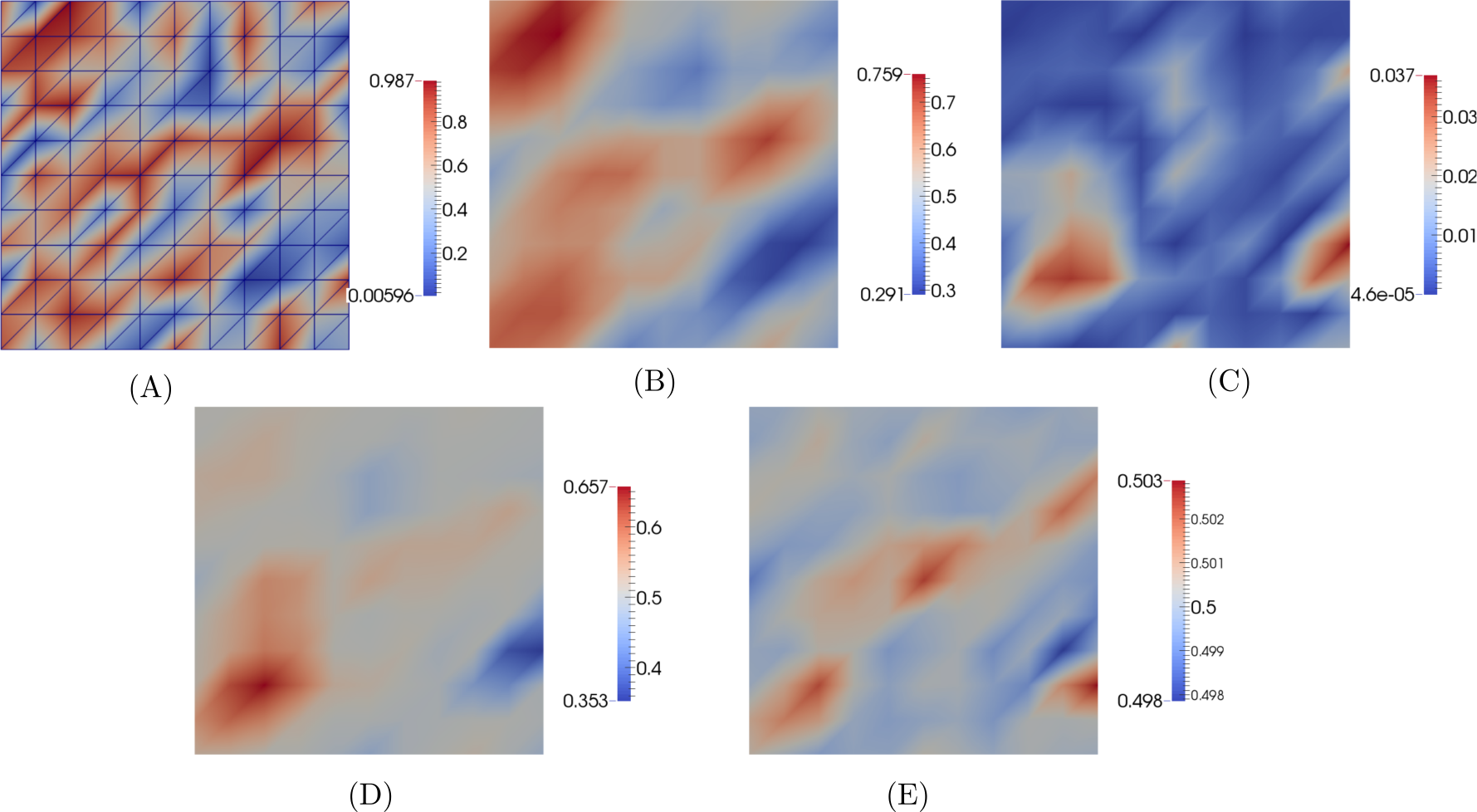
Figure 1: (A) The initial uniformly distributed random perturbation. (B) After applying smoothing to (A). (C) Sensitivity map based on 10 ensemble members. (D) Initial perturbation after smoothing and weighting by the importance map (C). (E) Initial perturbation after smoothing, weighting and orthogonalisation with respect to previous ensemble members and re-scaling.

3.2 Use of time windows, working backwards through time and concurrency

We split up the time domain into a number of non-overlapping intervals referred to as time windows, ensuring that there is an integer number of time steps within each time window. Once the unperturbed solution is available throughout time, the controls are also known at the beginning of each time window and are perturbed, thereby providing an ‘initial condition’ for each window. In this way a separate set of perturbations is applied to each time window. Due to these different sets of perturbations, the derivative $\frac{{\rm d}F}{{\rm d}\bm{\Psi}}$ (i.e. the sensitivity map) has to be mapped backwards in time through the time windows taking account of the change in the controls, $\bm{m}_{s}$ in each window. This mapping is now described.

Suppose that window $w$ is the time interval $[t^{b},t^{l})$, and window $w+1$ is the next time interval $[t^{l},t^{v})$, where $b$, $l$ and $v$ are indices that denote (global) time levels. Using the chain rule we can evaluate the derivative $\frac{{\rm d}F}{{\rm d}{\bm{m}}_{s}^{l}}$ in the current window, $w$, as follows

$$\left[\frac{{\rm d}F}{{\rm d}{\bm{m}}_{s}^{l}}\right]^{w}=\left[\frac{{\rm d}\bm{\Psi}^{l}}{{\rm d}{\bm{m}}_{s}^{l}}\right]^{w}\left[\frac{{\rm d}F}{{\rm d}{\bm{\Psi}}^{l}}\right]^{w+1}\,.$$ (35)

Applying the approximations we have used earlier (in equations (14), (15) and following (16)) at time level $l$ gives

$$\left[\widehat{\frac{{\rm d}F}{{\rm d}{\bm{m}}_{s}^{l}}}\right]^{w}=\left[(\widehat{{\bm{M}}}^{l}_{s})^{T}\right]^{w}\left[\widehat{\bm{g}}^{l}\right]^{w+1}\,,$$ (36)

where $\widehat{\bm{g}}^{l}$ has already been calculated in window $w+1$. For time window $w$, we can write the sensitivity map as follows

$$\widehat{\bm{g}}^{k}={\widehat{\bm{M}}_{s}^{k}}\left((\widehat{\bm{M}}_{s}^{k})^{T}\widehat{\bm{M}}_{s}^{k}\right)^{-1}\left(\left[\widehat{\frac{{\rm d}F}{{\rm d}{\bm{m}}_{s}^{l}}}\right]^{w}+\frac{{\rm d}F}{{\rm{d}}{\bm{m}}_{s}^{k}}\right),\;\;\forall k\in\left[b,l\right).$$ (37)

or using:

$$\frac{{\rm{d}}F}{{\rm{d}}{\bm{m}}_{s}^{k}}=\sum_{q=k}^{l-1}\frac{{\rm{d}}{\bm{\Psi}}^{q}}{{\rm{d}}{\bm{m}}^{k}_{s}}\frac{\partial F}{\partial{\bm{\Psi}}^{q}}+\frac{\partial F}{\partial{\bm{m}}^{k}_{s}},$$ (38)

then:

$$\widehat{\bm{g}}^{k}={\widehat{\bm{M}}_{s}^{k}}\left((\widehat{\bm{M}}_{s}^{k})^{T}\widehat{\bm{M}}_{s}^{k}\right)^{-1}\left(\left[\widehat{\frac{{\rm d}F}{{\rm d}{\bm{m}}_{s}^{l}}}\right]^{w}+\sum_{q=k}^{l-1}(\widehat{{\bm{M}}}^{q}_{s})^{T}\frac{\partial F}{\partial{\bm{\Psi}}^{q}}+\frac{\partial F}{\partial{\bm{m}}^{k}_{s}}\right),\;\;\forall k\in\left[b,l\right),$$ (39)

where all terms are now associated with time window $w$, hence the index $w$ is omitted. See Figure 2 for an illustration of this process. We show that using time windows can improve immensely the fidelity of the sensitivity maps for a given number of perturbations. This is because the perturbations can be more strongly focused on resolving the sensitivities in a particular time window, which results in the need for substantially fewer perturbations, see section 4.

Another key attribute of the time windows method is that each time window can be performed in isolation leading to “explicit time windows”. Using explicit time windows will have a certain loss of accuracy as $\widehat{\bm{g}}$ is no longer used to guide the generation of perturbed ensemble members. Nonetheless, explicit time windows introduce the potential to exploit parallelisation, as not only the ensemble members can be solved in parallel, but also the different time windows can be performed concurrently, enabling massive parallelisation.

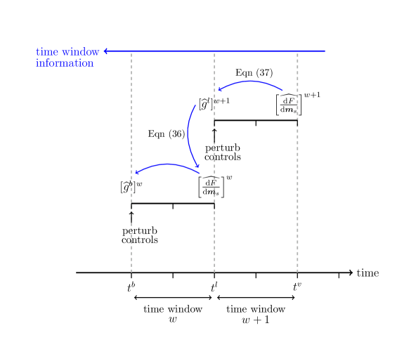
Figure 2: Two time windows are shown, window $w$, in which $t\in[t^{b},t^{l})$ and window $w+1$, in which $t\in[t^{l},t^{v})$ where $t^{b}$, $t^{l}$ and $t^{v}$ are global time levels. This illustrates the process of calculating the derivative $\frac{\widehat{\rm{d}F}}{\rm{d}\bm{m}^{l}_{s}}$ for window $w$ based on $\widehat{\bm{g}}^{l}$ of time window $w+1$, which is already known at this point due to the time windows being passed through in reverse order.

For ‘short’ time windows or when relying on a small number of perturbations, it may be useful to weight the perturbations with the previously calculated value of the sensitivity map from a future time window. This serves as an estimate of the initial value of $\widehat{\bm{g}}$ for the current time window as in the previously described goal-based approach (see section 3.1). For example, in time window $w$, the sensitivity map at the initial time of window $w$, $\widehat{\bm{g}}^{b}$, could be approximated by the sensitivity map at the initial time of window $w+1$, i.e.

$$\left[\widehat{\bm{g}}^{b}\right]^{w}\approx\left[\widehat{\bm{g}}^{l}\right]^{w+1}\,.$$ (40)

3.3 Re-orthogonalising through time

It is advantageous to orthogonalise the ensemble members for several reasons: (a) Each ensemble member will be given approximately equal priority in the generation of the sensitivity maps; (b) An independent set of ensemble members is guaranteed. Some random number generators have biases in them which may produce non-independent ensemble sets. This results in poor conditioning of the matrices that we invert within the procedure; (c) One can lose independence of the sets as time evolves, which means that some of the ensemble members are not contributing to the accuracy of the calculated $\widehat{\bm{g}}$. One way of addressing this issue is to use regularisation when forming the Moore-Penrose pseudo-inverse. That is introducing a positive diagonal matrix

$$\left(\widehat{\bm{M}}_{s}^{T}\widehat{\bm{M}}_{s}\right)^{-1}\rightarrow\left(\widehat{\bm{M}}_{s}^{T}\widehat{\bm{M}}_{s}+\epsilon_{s}{\bf I}\right)^{-1}$$ (41)

for some small $\epsilon_{s}$. An example of an equation that may be used to calculate $\epsilon_{s}$ is:

$$\epsilon_{s}=\frac{\alpha_{s}}{\cal E}\sum_{k=1}^{\cal E}\left(\widehat{\bm{M}}_{s}^{T}\widehat{\bm{M}}_{s}\right)_{kk}$$ (42)

in which $\alpha_{s}$ is a small number. We have used $\alpha_{s}=1\times 10^{-14}$ in the 1D applications where we have not used re-orthogonalisation or time windows. An alternative to using regularisation (equation (41)) is to re-orthogonalise the sets as the simulation progresses in time, as explained here.

We consider re-orthogonalising every time step in order to avoid losing independence of the set of ensemble members and thus being unable to invert the matrix $\widehat{\bm{M}}_{s}^{T}\widehat{\bm{M}}_{s}$. In practice one may re-orthogonalise every $N$ time steps (where $N>1$) to reduce the burden of this computation.

For a one level time discretisation, the solution at a particular time level can be thought of as the initial condition for the next time level, hence in this section the vector $\bm{m}$ containing the ‘initial conditions’ will now have a time index and satisfies

$$\bm{m}^{n}=\bm{\Psi}^{n}\,,$$ (43)

where $\bm{m}^{n}$ are the initial conditions which would lead to the discrete solution $\bm{\Psi}^{n+1}$. Suppose we have a solution vector at time level $n$, $\bm{\Psi}^{n}$. We set the deviation of this value from the unperturbed solution as the perturbation of the initial condition for the solution at the next time level

$$\Delta\bm{m}^{n}=\Delta\bm{\Psi}^{n}=\bm{\Psi}^{n}-\overline{\bm{\Psi}}^{n}\,.$$ (44)

It is at this point that we orthogonalise with respect to all other ensemble values at this time level

$$\Delta{}^{e}\tilde{\bm{m}}^{n}=\Delta{}^{e}\bm{m}^{n}-\sum_{k=1}^{e-1}\frac{(\Delta{}^{k}\bm{m}^{n})^{T}\Delta{}^{e}\bm{m}^{n}}{(\Delta{}^{k}\bm{m}^{n})^{T}\Delta{}^{k}\bm{m}^{n}}\,\Delta{}^{k}\bm{m}^{n}\,.$$ (45)

As before, for convenience, we wish to use the change of variables and so must also consider $\Delta{}^{e}\tilde{\bm{m}}^{n}_{s}$. Assuming, ${\Delta{}^{e}\bm{m}}_{s}^{n}$ is the set of perturbed ‘initial’ conditions at time level $n$ and $\Delta{}^{e}\tilde{\bm{m}}_{s}^{n}$ the orthogonalised set, then by definition

$$\Delta{}^{e}\tilde{\bm{m}}^{n}_{s}=\Delta{}^{e}\bm{m}^{n+1}_{s}\,,$$ (46)

which leads to the result

$$\widehat{\frac{{\rm d}F}{{\rm d}\tilde{\bm{m}}_{s}^{n}}}=\widehat{\frac{{\rm d}F}{{\rm d}{\bm{m}}_{s}^{n+1}}}\,.$$ (47)

This is true because, at each time step, the change of variables is such that the controls $\Delta{}^{e}\bm{m}_{s}$ have the properties given in equation (10). At this stage we orthogonalise and must relate derivatives with respect to $\bm{m}^{n}_{s}$ and $\tilde{\bm{m}}^{n}_{s}$ by the following (valid for time level $n$):

$$\widehat{\frac{{\rm d}F}{{\rm d}{\bm{m}}_{s}^{n}}}=\frac{{\rm d}\tilde{\bm{m}}_{s}^{n}}{{\rm d}{\bm{m}}_{s}^{n}}\widehat{\frac{{\rm d}F}{{\rm d}\tilde{\bm{m}}_{s}^{n}}}=:({{\bm{V}}^{n}})^{-T}\widehat{\frac{{\rm d}F}{{\rm d}\tilde{\bm{m}}_{s}^{n}}}$$ (48)

In order to calculate the sensitivity map, we need to be able to calculate $\bm{V}$. To derive an expression we apply the chain rule to the derivative of the solution variables giving

$$\frac{{\rm d}\bm{\Psi}^{n}}{{\rm d}{\bm{m}}^{n}_{s}}\frac{{\rm d}{\bm{m}}^{n}_{s}}{{\rm d}\tilde{\bm{m}}^{n}_{s}}=\frac{{\rm d}\bm{\Psi}^{n}}{{\rm d}{\bm{m}}^{n}_{s}}{\bm{V}}^{n}=\frac{{\rm d}\bm{\Psi}^{n}}{{\rm d}\tilde{\bm{m}}^{n}_{s}}\,.$$ (49)

Combining this for all ensemble members and using the approximation ${\bm{M}}_{s}^{n}\approx\widehat{\bm{M}}_{s}^{n}$, we assume that

$$\widehat{\bm{M}}_{s}^{n}{\bm{V}}^{n}=\widetilde{\bm{M}}_{s}^{n}.$$ (50)

With the identity $(\widetilde{\bm{M}}_{s}^{n})^{T}\widetilde{\bm{M}}_{s}^{n}=\bm{I}$ in mind, we pre-multiply the above matrix equation by $(\widetilde{\bm{M}}_{s}^{n})^{T}$ to give

$$\bm{V}^{n}=\left((\widetilde{\bm{M}}_{s}^{n})^{T}\widehat{\bm{M}}_{s}^{n}\right)^{-1},$$ (51)

and thus:

$$({\bm{V}}^{n})^{-T}=\left((\widetilde{\bm{M}}_{s}^{n})^{T}\widehat{\bm{M}}_{s}^{n}\right)^{T}.$$ (52)

So in a practical algorithm one simply updates $\widehat{\frac{{\rm d}F}{{\rm d}{\bm{m}}_{s}^{n}}}$ using equations (47) and (48) working backwards through time from the last time level:

$${\bm{m}}_{s}^{n+1}\widehat{\frac{{\rm d}F}{{\rm d}{\bm{m}}_{s}^{n}}}=\left(\bm{V}^{n}\right)^{-T}\widehat{\frac{{\rm d}F}{{\rm d}\tilde{\bm{m}}_{s}^{n}}}=\left(\bm{V}^{n}\right)^{-T}\widehat{\frac{{\rm d}F}{{\rm d}{\bm{m}}_{s}^{n+1}}},$$ (53)

and then applies equation (21) to obtain the sensitivity map $\widehat{\bm{g}}^{n}$ at time level $n$.

3.4 Typical algorithm for ensemble sensitivity calculation for time dependent problems

A typical algorithm for the goal-based approach outlined in section 3.1 can be seen in Algorithm 1. Extending this to include time windows (section 3.2) is done in Algorithm 2. Both of these algorithms use two functions, SolveEnsembles and CalculateSensitivityMap described in Algorithms 3 and 4 respectively. All other functions are not described as their form is implied by the function name. The function SolveEnsembles inlcudes the smoothing, weighting and orthogonalising of the perturbations on line 3. The function CalculateSensitivityMap shows how the sensitivity map is calculated, using all ensemble members for whichever time levels are desired. The inputs and outputs of the functions are shown in mathematical notation in order to facilitate comparison with the equations.

Algorithm 1 Calculate $\widehat{\bm{g}}$ using the goal-based approach (section 3.1).

1:!! Run unperturbed forward model

2:$\overline{\bm{m}}$ = ReadInitialCondition( )

3:$\overline{\bm{\Psi}}$ = RunForwardModel($\overline{\bm{m}}$)

4:$\overline{\bm{F}}$ = CalculateF($\overline{\bm{\Psi}}$)

5:

6:!! Initialise sensitivity map vector

7:$\widehat{\bm{g}}^{0}=\bm{1}$

8:!! Create the perturbations and solve the forward model

9:$({}^{1}\bm{\Psi},{}^{2}\bm{\Psi},\ldots,{}^{\cal{E}}\bm{\Psi}),({}^{1}F,{}^{2}F,\ldots,{}^{\cal{E}}F)$=SolveEnsembles($\widehat{\bm{g}}^{0}$, $\overline{\bm{m}}$)

10:

11:!! Calculate the derivative of $F$ with respect to the controls, equation (14)

12:$\widehat{\frac{\rm{d}F}{\rm{d}\bm{m}_{s}}}$ = Calculate dFdms(${}^{1}F,{}^{2}F,\ldots,{}^{\cal{E}}F,\overline{F}$)

13:

14:!! Calculate the sensitivity map at each desired time level based on all $\cal{E}$ ensemble members, equation (21)

15:$(\widehat{\bm{g}}^{0},\widehat{\bm{g}}^{1},\ldots,\widehat{\bm{g}}^{n})$=CalculateSensitivityMap($({}^{1}\bm{\Psi},{}^{2}\bm{\Psi},\ldots,{}^{\cal{E}}\bm{\Psi}),({}^{1}F,{}^{2}F,\ldots,{}^{\cal{E}}F)$, $\widehat{\frac{\rm{d}F}{\rm{d}\bm{m}_{s}}}$, $\overline{\bm{\Psi}}$, $\overline{F}$)

Algorithm 2 Calculate $\widehat{\bm{g}}$ using the goal-based approach and time windows (sections 3.1 and 3.2)

1:!! Run unperturbed forward model

2:$\overline{\bm{m}}$ = ReadInitialCondition( )

3:$\overline{\bm{\Psi}}$ = RunForwardModel($\overline{\bm{m}}$)

4:$\overline{\bm{F}}$ = CalculateF($\overline{\bm{\Psi}}$)

5:

6:!! Initialise sensitivity map vector

7:$\widehat{\bm{g}}^{\text{init}}=\bm{1}$

8:for window $w=\,1$ to $W$ in reverse do

9:     $[{}^{1}\bm{\Psi},{}^{2}\bm{\Psi},\ldots,{}^{\cal{E}}\bm{\Psi}]^{w},[{}^{1}F,{}^{2}F,\ldots,{}^{\cal{E}}F]^{w}$ = SolveEnsembles($[\widehat{\bm{g}}^{\text{init}}]^{w},\overline{\bm{m}}$)

10:     

11:     !! Calculate the derivative of $F$ with respect to the controls using …

12:     if $w==W$ then

13:         !! …equation (14)

14:         $\left[\widehat{\frac{\rm{d}F}{\rm{d}\bm{m}_{s}}}\right]^{w}$ = Calculate dFdms($\left[{}^{1}F,{}^{2}F,\ldots,{}^{\cal{E}}F\right]^{w},\overline{F}$)

15:     else

16:         !! …equations (15) and (36)

17:         $\widehat{\bm{M}}_{s}^{n}$= Calculate d$\Psi$dm(${}^{1}\bm{\Psi}^{n},{}^{2}\bm{\Psi}^{n},\ldots,{}^{\cal{E}}\bm{\Psi}^{n},\overline{\bm{\Psi}}$)

18:         $\left[\widehat{\frac{\rm{d}F}{\rm{d}\bm{m}_{s}}}\right]^{w}=[\widehat{\bm{M}}_{s}]^{w}[\widehat{\bm{g}}]^{w+1}$

19:     end if

20:     

21:     !! Calculate the sensitivity map based on all $\cal{E}$ ensemble members, equation (39)

22:     $(\widehat{\bm{g}}^{0},\widehat{\bm{g}}^{1},\ldots,\widehat{\bm{g}}^{n})$=CalculateSensitivityMap($({}^{1}\bm{\Psi},{}^{2}\bm{\Psi},\ldots,{}^{\cal{E}}\bm{\Psi})$, $({}^{1}F,{}^{2}F,\ldots,{}^{\cal{E}}F)$,$\widehat{\frac{\rm{d}F}{\rm{d}\bm{m}_{s}}}$,$\overline{\bm{\Psi}}$, $\overline{F}$)

23:end for

Algorithm 3 Create the perturbations and solve the ensemble members

1:function SolveEnsembles($\bm{\widehat{g}^{0}}$, $\overline{\bm{m}}$)

2:     for ensemble $e=\,1$ to $\cal{E}$ do

3:         !! Create perturbations

4:         $\Delta{}^{e}\bm{m}$ = GetPerturbation($\widehat{\bm{g}}^{0}$) !! Using equations (29), (31), (32) and (34)

5:         ${}^{e}\bm{m}$ = $\overline{\bm{m}}+\Delta{}^{e}\bm{m}$

6:         !! Solve the forward model

7:         ${}^{e}\bm{\Psi}$ = RunForwardModel(${}^{e}\bm{m}$)

8:         ${}^{e}F$ = CalculateF(${}^{e}\bm{\Psi}$)

9:         

10:         !! Calculate sensitivity map for time level 0 based on ensemble members $1$ to $e$

11:         $\widehat{\bm{M}}^{0}$ = Calculate d$\Psi$dm(${}^{1}\bm{\Psi}^{0},{}^{2}\bm{\Psi}^{0},\ldots,{}^{e}\bm{\Psi}^{0},\overline{\bm{\Psi}}$) !! equation (15)

12:         $\widehat{\frac{\rm{d}F}{\rm{d}\bm{m}_{s}}}$ = Calculate dFdms(${}^{1}F,{}^{2}F,\ldots,{}^{e}F,\overline{F}$) !! equation (14)

13:         $\widehat{\bm{g}}^{0}$ = CalculateSensitivityMapTimeLevel($\widehat{\bm{M}}^{0},\widehat{\frac{\rm{d}F}{\rm{d}\bm{m}_{s}}}$) !! equation (21)

14:     end for

15:     return $({}^{1}\bm{\Psi},{}^{2}\bm{\Psi},\ldots,{}^{\cal{E}}\bm{\Psi}),({}^{1}F,{}^{2}F,\ldots,{}^{\cal{E}}F)$

16:end function

Algorithm 4 Calculates the sensitivity map

1:function CalculateSensitivityMap($({}^{1}\bm{\Psi},{}^{2}\bm{\Psi},\ldots,{}^{\cal{E}}\bm{\Psi}),({}^{1}F,{}^{2}F,\ldots,{}^{\cal{E}}F)$, $\widehat{\frac{\rm{d}F}{\rm{d}\bm{m}_{s}}}$, $\overline{\bm{\Psi}}$, $\overline{F}$)

2:     for each time level $n$ do

3:         $\widehat{\bm{M}}^{n}$= Calculate d$\Psi$dm(${}^{1}\bm{\Psi}^{n},{}^{2}\bm{\Psi}^{n},\ldots,{}^{\cal{E}}\bm{\Psi}^{n},\overline{\bm{\Psi}}$) !! equation (15)

4:         $\widehat{\bm{g}}^{n}$ = CalculateSensitivityMapTimeLevel($\widehat{\bm{M}}^{n},\widehat{\frac{\rm{d}F}{\rm{d}{m}}_{s}}$) !! equation (21)

5:     end for

6:     return $(\widehat{\bm{g}}^{0},\widehat{\bm{g}}^{1},\ldots,\widehat{\bm{g}}^{n})$

7:end function

4 Results

Problems from different subject areas are tackled using different codes to prove the robustness of the presented method. First, it is tested in a 1D code for advection (see section 4.1). Next, the method is used to analyse a 2D system in which we model the advection of a tracer (see section 4.2) with the code Fluidity [34, 1, 46] and using the flux limited advection method [13]. This advection method uses, as the high order solution, a Finite Element Galerkin projection of the control volume solution with linear triangular elements. Finally, the formulation is used to study the behaviour of a non-linear multi-phase porous media flow in a 3D heterogeneous media (section 4.3) using ICFERST [17, 13, 37].

For test cases 4.1 and 4.2 we solve the advection equation:

$$\frac{\partial c}{\partial t}+\bm{u}\cdot\nabla c=0\,,$$ (54)

in which $\bm{u}=1$ for 1D, $\bm{u}=(1,0)$ for 2D, and where $c$ is the concentration of the tracer.

For readability, a brief summary of the equations to solve for multi-phase porous media flow (test case 4.3) are presented. A more complete description of the formulation has been published [17, 13, 37]. Darcy’s equation is as follows:

$$\mu_{\alpha}S_{\alpha}\left(\mathcal{K}_{{r}_{\alpha}}\mathbf{K}\right)^{-1}\bm{u}_{\alpha}=-\nabla p+{\bm{s}_{u}}_{\alpha},$$ (55)

in which $\bm{u}_{\alpha}$ is the velocity of phase $\alpha$, $p$ is the global pressure of the system and $\bm{s}_{{u}_{\alpha}}$ is a source term; here no sources are considered. $\mathbf{K}$ is the permeability tensor, and $\mathcal{K}_{{r}_{\alpha}}$, $\mu_{\alpha}$ and $S_{\alpha}$ are the relative permeability, viscosity and saturation of phase $\alpha$ respectively.

The saturation equation for incompressible flow is:

$$\phi\displaystyle\frac{\partial S_{\alpha}}{\partial t}+\nabla\cdot\left({\bm{u}}_{\alpha}S_{\alpha}\right)=0,$$ (56)

in which $\phi$ is the porosity.

The system of equations is closed by ensuring that the phase saturations sum to one:

$$\sum\limits_{\alpha=1}^{n}S_{\alpha}=1,$$ (57)

$n$ being the number of phases. For the relative permeability, the Brooks-Corey model [5] is used

$$k_{rw}\left(S_{w}\right) = \left(\frac{S_{w}-S_{wirr}}{1-S_{wirr}-S_{nwr}}\right)^{n_{w}},$$ (58)

$$k_{rnw}\left(S_{nw}\right) = \left(\frac{S_{nw}-S_{nwr}}{1-S_{wirr}-S_{nwr}}\right)^{n_{nw}},$$ (59)

in which $n_{w}$ and $n_{nw}$ are the exponents for the wetting and non-wetting phases respectively. $S_{nwr}$ is the irreducible non-wetting phase saturation and $S_{wirr}$ is the irreducible wetting phase saturation.

4.1 1D advection equation test

Equation (54) is solved with an initial condition of $c=0$. The number of cells is set to ${\cal N}=101$ and the domain size is $100$ with the cell spacing equal to $\Delta x=1$. The time-step size is set to $\Delta t=0.1$, the default number of equally-sized time steps is ${\cal N}_{t}=600$ and a forward Euler scheme is used. In this 1D test, the functional that we use in forming the sensitivities to the solution variables ($c_{i}^{n}$) is

$$F=c_{k}^{{\cal N}_{t}}\;\;{\rm with}\;\;k={\left\lfloor{0.85{\cal N}}\right\rfloor}.$$ (60)

That is, the concentration at the final time level ${{\cal N}_{t}}$ and at cell $\left\lfloor{0.85{\cal N}}\right\rfloor$ which is the nearest integer from below to $0.85{\cal N}$. The cells are ordered from left to right with increasing $x$-coordinate. Thus the exact sensitivities at the end of time $n={{\cal N}_{t}}$ are:

$$\frac{\rm{d}F}{\rm{d}c_{i}^{{\cal N}_{t}}}=1,\;\;{\rm if}\;\;i=\left\lfloor{0.85{\cal N}}\right\rfloor\;\;{\rm and}\;\;\frac{\rm{d}F}{\rm{d}c_{i}^{{\cal N}_{t}}}=0\;\;{\rm if}\;\;i\neq\left\lfloor{0.85{\cal N}}\right\rfloor.$$ (61)

The number of smoothing iterations is set to $25$. To further explore the effectiveness of the presented method we use, either, an upwind differencing scheme (linear) or a Normalised Variable Diagram [23] (NVD) flux-limiting differencing scheme (non-linear). The high order scheme within the NVD method is the diamond differencing scheme (a mid-point scheme) and the NVD is such that diamond differencing is used as much as possible while not violating the Total Variational Diminishing criteria.

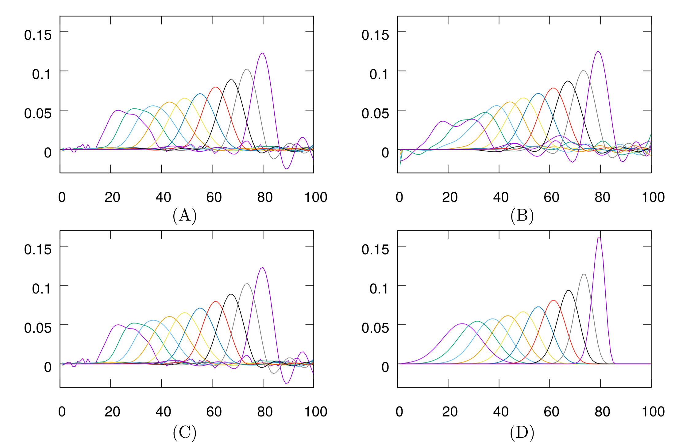
Figure 3: The advection of sensitivities backwards through time using the upwind scheme. The $x$-axis shows the $x$ -coordinate, the $y$-axis shows the amplitude of the sensitivities. Ten different time instances (represented by different curves) equally spaced from beginning to the end of the time are plotted. (A) results using the goal-based approach, performing 10 perturbations and without re-orthogonalisation. (B) results without the goal-based approach, performing 10 perturbations and without re-orthogonalisation. (C) results using the goal-based approach, performing 10 perturbations and with re-orthogonalisation. (D) results using the goal-based approach, performing 101 perturbations and with re-orthogonalisation.

Figure 3 shows the results of advecting the sensitivities backwards through time. Upwind differencing is used in the forward model. Ten equally-spaced time instances (spanning the time domain) are plotted. Each curve represents a different time instance and displays the sensitivities ($\widehat{\bm{g}}^{n}$) at that time instance $n$. Hence, the peak of each curve occurs at a different position. Figure 3 (A) displays the results using the goal-based approach, 10 perturbations and without re-orthogonalisation. Figure 3(B) displays the results using 10 perturbations without the goal-based approach and without re-orthogonalisation. Comparing these figures is effectively comparing the methods known in the literature, see section 2.3, with our goal-based approach, section 3.1. It is clearly seen that without the goal-based approach, Figure 3(B), there are more oscillations in the sensitivity map than with the goal-based approach, Figure 3(A). Figure 3(C) is obtained using the goal-based approach, 10 perturbations and re-orthogonalisation. There is little difference between Figures 3(C) and 3(A), because, for such a low number of perturbations, the re-orthogonalisation has little effect as the perturbations naturally remain independent to one another. Finally, Figure 3(D) displays the results using the goal-based approach, 101 perturbations and re-orthogonalisation. Equivalent to direct sensitivity analysis, the results for 101 perturbations are effectively the “true” numerical sensitivities. These sensitivities are in effect exact because, for the linear scheme, the resulting sensitivites are independent of the size of the perturbations. We have also varified the code and approach by directly perturbing each variable in order to produce the exact sensitivites which are identical to those shown in Figure 3(D). It can be seen that with only 10 perturbations a good result can be obtained (compare Figure 3(A) or (C) with Figure 3(D)).

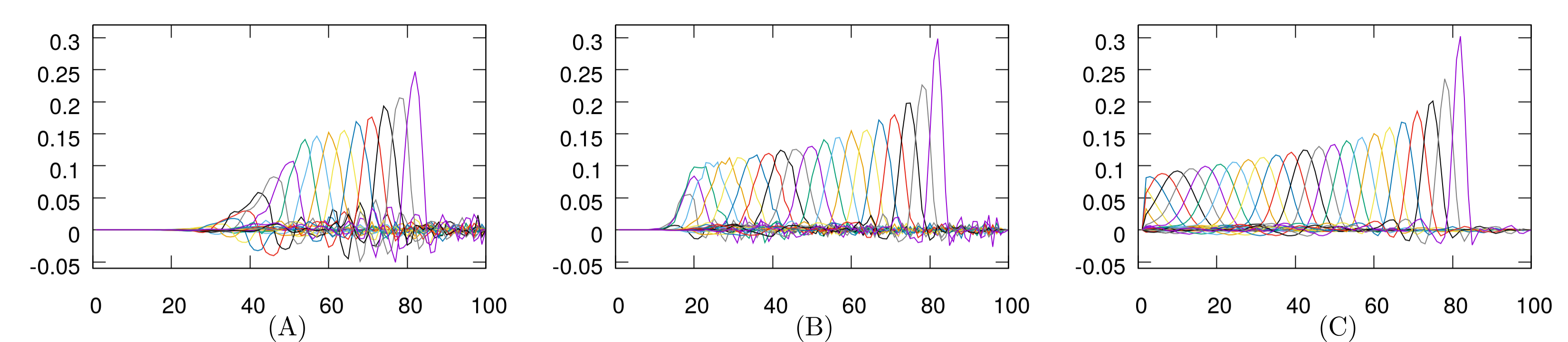
Figure 4: Sensitivity results using the non-linear NVD flux-limiting scheme, ${\cal N}_{t}=3600$ time steps with the goal-based approach and re-orthogonalisation. (A) results performing $20$ perturbations. (B) results performing $40$ perturbations. (C) results performing $101$ perturbations. The $x$-axis shows the $x$-coordinate, the $y$-axis shows the amplitude of the sensitivities.

Figure 4 shows the results using the non-linear NVD flux-limiting scheme for ${\cal N}_{t}=3600$ time steps. The longer run time means that the information travels 3.6 times the length of the domain. Here, the goal-based approach and re-orthogonalisation are used in all three cases. This test demonstrates the benefits of re-orthogonalisation, as without it, the perturbations would be advected out of the domain therefore making it impossible to calculate a sensitivity map. The results are less dissipative than in the previous case due to the non-linear scheme used. Figure 4 (C) displays the results using $101$ perturbations and represents the true numerical sensitivities through time. Figures 4 (A) and (B) show the results using $20$ and $40$ perturbations respectively. It can be seen how, in this case, with $20$ perturbations, the results are not as good as before with $10$. However, the results are good enough to show the sensitivities developing over the latter half of the numerical simulation. These results are much improved when using $40$ iterations, showing the sensitivities over the majority of the numerical domain.

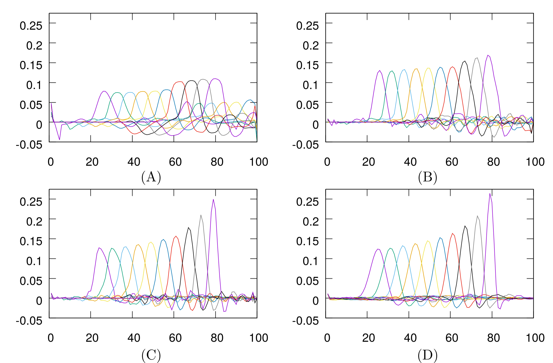
Figure 5: Sensitivity results using the non-linear NVD flux-limiting scheme, the goal-based approach and re-orthogonalisation. (A) results performing $5$ perturbations. (B) results performing $10$ perturbations. (C) results performing $20$ perturbations. (D) results performing $101$ perturbations. The $x$-axis shows the $x$-coordinate, the $y$-axis shows the amplitude of the sensitivities.

Figure 5 shows the results of using the non-linear NVD flux-limiting scheme, the goal-based approach and re-orthogonalisation for 5, 10, 20 and 101 perturbations in Figure 5 (A), (B), (C) and (D) respectively. Even with 5 perturbations the sensitivities start to emerge and are well represented. With 10 perturbations it can be seen that the results are improved. With 20 perturbations the results are close to the final result obtained with 101 perturbations, taken to be the true sensitivities.

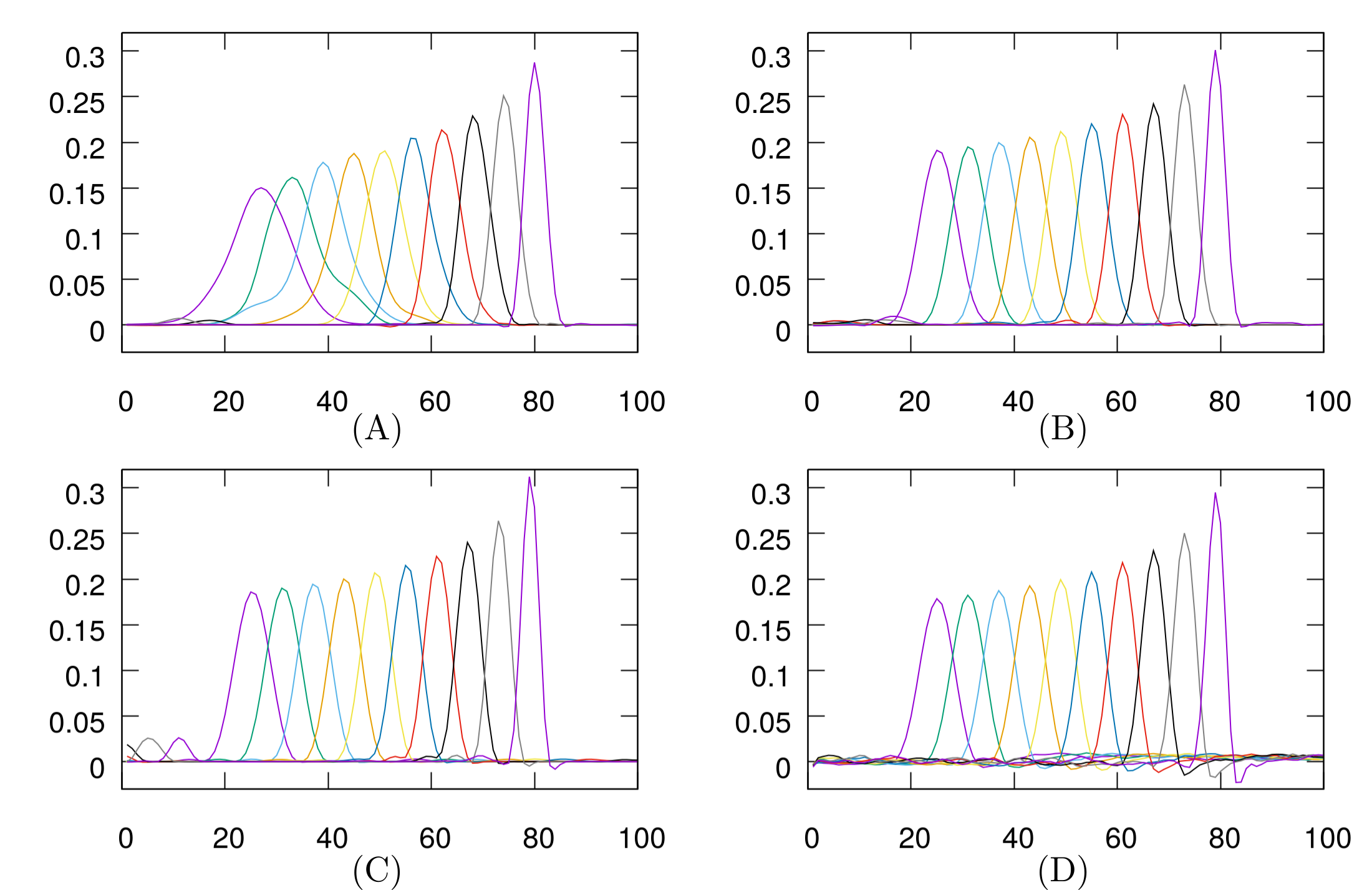
Figure 6: Sensitivity results using the non-linear NVD flux-limiting scheme, the goal-based approach and time windows. (A) results performing $5$ perturbations. (B) results performing $10$ perturbations. (C) results performing $20$ perturbations. (D) results performing $101$ perturbations. The $x$-axis shows the $x$-coordinate, the $y$-axis shows the amplitude of the sensitivities.

In Figure 6 we repeat the test shown in Figure 5, but now using time windows of size equal to one time step and working backwards through time. Since we are using time windows there is no need to use re-orthogonalization. Figures 6 (A), (B), (C) and (D) have been obtained with 5, 10, 20 and 101 perturbations respectively. It can be seen that even with 5 perturbations the results are excellent, representing the sensitivities well and minimising the oscillations.

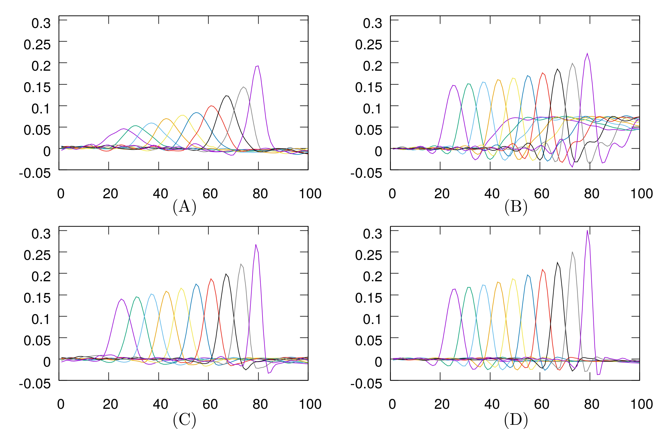
Figure 7: Sensitivity results using the non-linear NVD scheme, the goal-based approach (unless otherwise stated), re-orthogonalisation and explicit time windows. (A) results performing $20$ perturbations. (B) results performing $30$ perturbations without the goal-based approach. (C) results performing $30$ perturbations. (D) results performing $50$ perturbations. The $x$-axis shows the $x$-coordinate, the $y$-axis shows the amplitude of the sensitivities.

The test reported in Figures 5 and 6 is repeated once again using explicit time windows (that can be calculated concurrently), with the goal-based approach unless stated, for 25, 30 (without goal-based), 30 and 50 perturbations and shown in Figure 7 (A), (B), (C) and (D) respectively. In this case, at least 25 perturbations are required to obtain meaningful results. Moreover, for 30 perturbations, not using the goal-based approach results in a much worse sensitivity map, seen by comparing Figure 7 (B) with (C). On comparing these results with those shown in Figure 6, it can be seen that explicit time windows require at least twice as many perturbations than standard time windows. However, explicit time windows do provide the opportunity to exploit parallelisation as all the perturbations and time windows can be performed at the same time. In this case 600 time windows are determined concurrently. Therefore, requiring more perturbations to obtain good results can easily be overcome by using the increased parallel capabilities introduced by this approach.

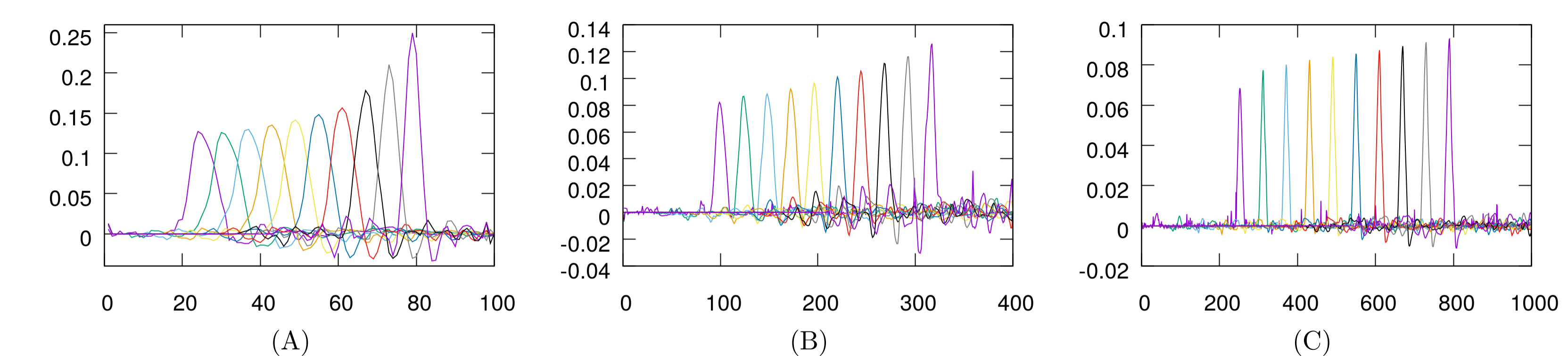
Figure 8: Sensitivity results using the non-linear NVD scheme and the goal-based approach, where the initial perturbation is weighted by $\widehat{\bm{g}}^{0},$ using only $20$ perturbations for three different meshes: $101$, $401$ and $1001$ cells, labelled (A), (B) and (C) respectively. The $x$-axis shows the $x$-coordinate, the $y$-axis shows the amplitude of the sensitivities.

Figure 8 shows the results using the goal-based approach with only $20$ perturbations for different meshes ($101$, $401$ and $1001$ cells). For each mesh, the time step is changed accordingly to ensure a constant Courant number. In all the cases, the results obtained are accurate. The sensitivities become sharper as the mesh is refined. We remark that resolving a numerical delta function is extremely demanding for ensemble methods, yet here, with just 20 perturbations, the back-propagation of the sensitivities is well resolved even when using a very fine mesh (which increases the number of controls). It should be noted that the magnitude of the sensitivites decreases with increasing resolution. This is because, although the magnitude of the sensitivity maps begins with a magnitude of 1 in one cell (0 in all others), see equation (61), it quickly reduces (at least initially) as it spreads out and advects backwards in time.

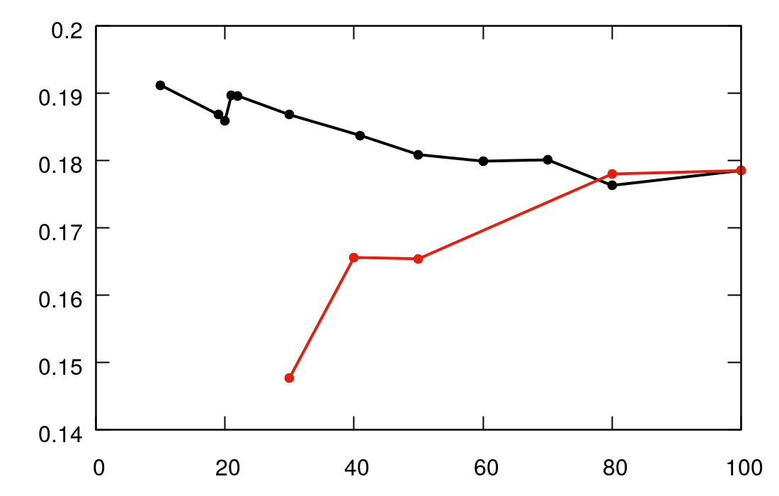
Figure 9: The maximum value of $\widehat{\bm{g}}$ at $t=0$ is plotted against number of perturbations for results obtained using re-orthogonalisation, with (black) and without (red) $\widehat{\bm{g}}$ weighting the initial perturbations. The number of cells is $101$ for this problem, and the non-linear NVD scheme is used.

From these numerical simulations it can be concluded that the goal-based approach is central to obtaining accurate sensitivity maps with fewer perturbations. Figure 9 shows the convergence of the sensitivities for different numbers of perturbations, both with and without the goal-based approach. It should be noted that although the aim of some work is to have a degree of ensemble spread [14], our aim is to explicitly have the most accurate sensitivities of the goal. Without the goal-based approach, results cannot be obtained unless a minimum of 30 perturbations are performed. Moreover, with 30 perturbations the results are worse than the case for the goal-based approach with 10 perturbations. As the number of perturbations is increased, the case using the goal-based approach consistently provides better results until reaching 80 perturbations (of a maximum of 101), when not using the goal-based approach is marginally better.

4.2 2D advection equation test

The governing equations for the 2D advection test are given in equation (54). For this test the velocity is set to $\bm{u}=(1,0)^{T}$, the domain size is 5 by 5 with a structured mesh of $100$ linear triangular elements and $121$ nodes (see Figure 1), the time step is set to 0.125 and the simulations are run from $t=0$ to $t=3.5$. The initial condition is $c(x,y,t=0)=0.5$, and the boundary conditions are $c(0,y,t)=0.5$, $c(5,y,t)=0$, $c(x,5,t)=0$ and $c(x,0,t)=0$. The functional in this problem is defined to be the concentration at the end of time ($n={{\cal N}_{t}}$) at the point $(4,1.5)$ (indicated by a black diamond in Figure 10 top-left). The analytical adjoint would be a dirac delta function which would move across the domain along the line $y=1.5$. The numerical solution suffers from dissipation, so the sensitivity map (i.e. the numerical adjoint) will reflect this, spreading out and reducing in magnitude.

Results are shown for one time window of 3.5 time units and seven time windows, each window of length 0.5 time units. For the one time-window case no special features are enabled (e.g. smoothing, weighing, orthogonalisation etc.). For the seven time-window case, we weight the intial conditions with the sensitivity map available at the time, we orthogonalise and we pass down the value of the sensitivity map from one window to the previous. In both cases we use three smoothing iterations. Figure 10 shows results based on an ensemble size of 20. The plots in the left column pertain to one time window, those on the right, to seven time windows. The plots at the top are taken at the initial time $t=0$, those in the middle correspond to $t=1.75$ and those at the bottom are taken at the final time, $t=3.5$. The results for seven time windows show clearer sensitivity maps with less oscillation especially at earlier times. The peak value of the sensitivities is also larger for the seven window case.

Figure 11 shows results based on an ensemble size of 40. Again, the plots at the top are taken at the initial time $t=0$, those in the middle correspond to $t=1.75$ and those at the bottom are taken at the final time, $t=3.5$ with plots relating to one time window (and no additional features) on the left, seven time windows and all features on the right. Similar conclusions can be drawn to the previous case of 20 ensemble members, i.e. that the results for seven time windows show clearer sensitivity maps with less oscillation especially at earlier times, and the seven time-window case has a higher peak value. When using one time window and no additional features, the sensitivity maps are still not accurate even with an ensemble size of 40. When using seven time windows and all the features, an ensemble size of 20 may be enough (for some applications) to yield accurate sensitivities throughout time.

Comparing Figure 10 (left) and Figure 11 (left) shows the need to re-orthogonalise through time, as using larger ensemble sizes actually increases the noise seen in the sensitivity maps. This occurs due to the system becoming ill-posed, as time evolves, some random perturbations become similar to previously used perturbations. This can be solved either by introducing regularisation, by perturbing the boundary condition on the left of the domain or by ensuring that all the perturbations are orthogonal with respect to one another, which also increases the efficiency of the method.

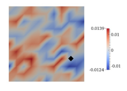
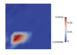
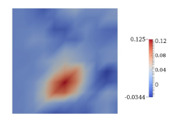
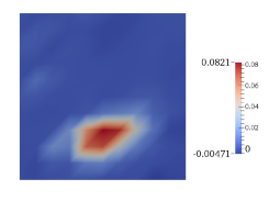
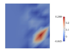
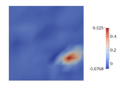
Figure 10: Results on the left show the sensitivity map generated with no smoothing, no weighting, no orthogonalisation and by using one time window. Results on the right are generated by smoothing the perturbations, weighting them with the sensitivity map available at that time, orthogonalising and by using seven time windows. The sensitivity map is shown at times $t=0$ (top), $t=1.75$ (middle) and $t=3.5$ (bottom). The size of ensemble is 20.

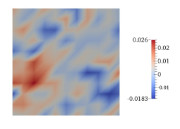
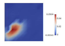
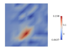
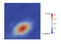
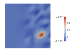
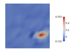
Figure 11: Results on the left show the sensitivity map generated with no smoothing, no weighting, no orthogonalisation and by using one time window. Results on the right are generated by smoothing the perturbations, weighting them with the sensitivity map available at that time, orthogonalising and by using seven time windows. The sensitivity map is shown at times $t=0$ (top), $t=1.75$ (middle) and $t=3.5$ (bottom). The size of ensemble is 40.

4.3 3D porous media test case

Here, the presented method is tested against a 3D multi-phase porous media flow. This test case has been chosen to explore the behaviour of the presented methodology against a highly non-linear system. The non-linearity arises from the relationship between the saturation and the relative permeability resulting in a non-linear correlation between the velocity of the phases and the saturation [20]. In this test case the saturation field is perturbed, as it affects the behaviour of the other fields. It is important to note that the amplitude of the perturbations performed is higher in this case. The range of the perturbations, in this case, is $0.1$, which is consistent with the perturbation amplitudes required to trigger viscous fingering [19].

The porous medium consists of a box reservoir ($\mathbf{K}_{out}=1$ dimensionless permeability units) with a low permeable inclusion ($\mathbf{K}_{out}=10^{-5}$ dimensionless permeability units) in the centre (Figure 12 (A)); the porosity is homogeneous in the whole domain and $\phi=0.2$. The domain is initially saturated by the non-wetting phase with a saturation equal to ($1-S_{wirr}$). The wetting phase is injected (at a rate of $0.2$) over the left boundary displacing the non-wetting phase towards the right boundary; the other boundaries are closed to flow. The viscosity ratio of the phases is $1$. The time-step size is set to $0.025$ and the final time is set to $0.375$.

Figure 12 (B-D) shows the forward simulation of this test case. The flow goes around the low permeable inclusion. The point of interest is located at the black diamond in Figure 12 (D) ($x=0.773$, $y=0.5$, $z=0.59$), this location is chosen to force a flowpath that is not linear. The time of interest is at the end of time and therefore the functional $F$ is defined as the phase 1 saturation at the point and time of interest.

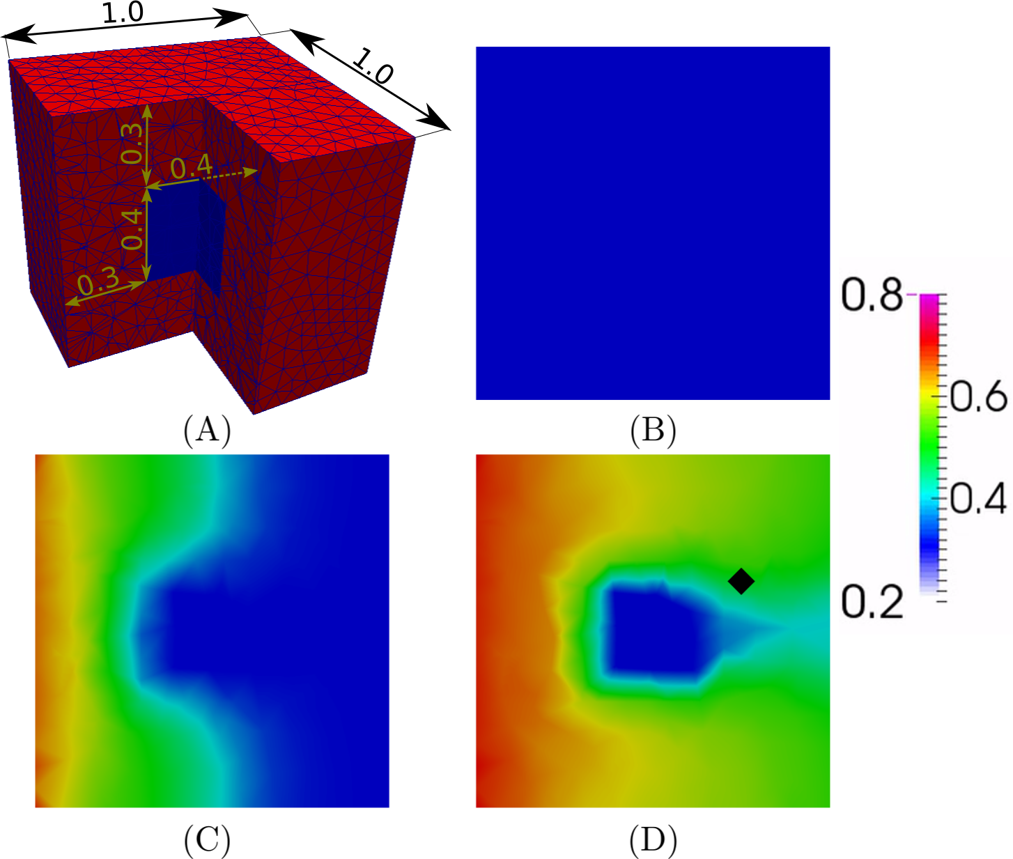
Figure 12: (A) Slice of the 3D domain showing the internal inclusion; domain dimensions, mesh (9879 elements) and permeability map are displayed. (B) (C) and (D) show the wetting saturation obtained from the forward model at three time instances. The diamond in (D) marks the point of interest used to create the sensitivity maps.

Two sets of experiments are performed, both with ensemble sizes of 20 and 40. One set is generated by performing 5 smoothing iterations, weighting with the sensitivity map available at that time, orthogonalising and by using 4 time windows. The other set is generated without using these techniques. In the latter case, none of these results provided a meaningful sensitivity map, and therefore the results are not included. Figure 13 shows the sensitivity maps, the left column displays the results using an ensemble size of 20 and the right column, using an ensemble size of 40. It can be seen that, in this case, an ensemble size of 20 is not enough to provide a very reliable sensitivity map. Nonetheless, for an ensemble size of 40 the results are very accurate, as they show well-defined regions with little or no oscillation in the results.

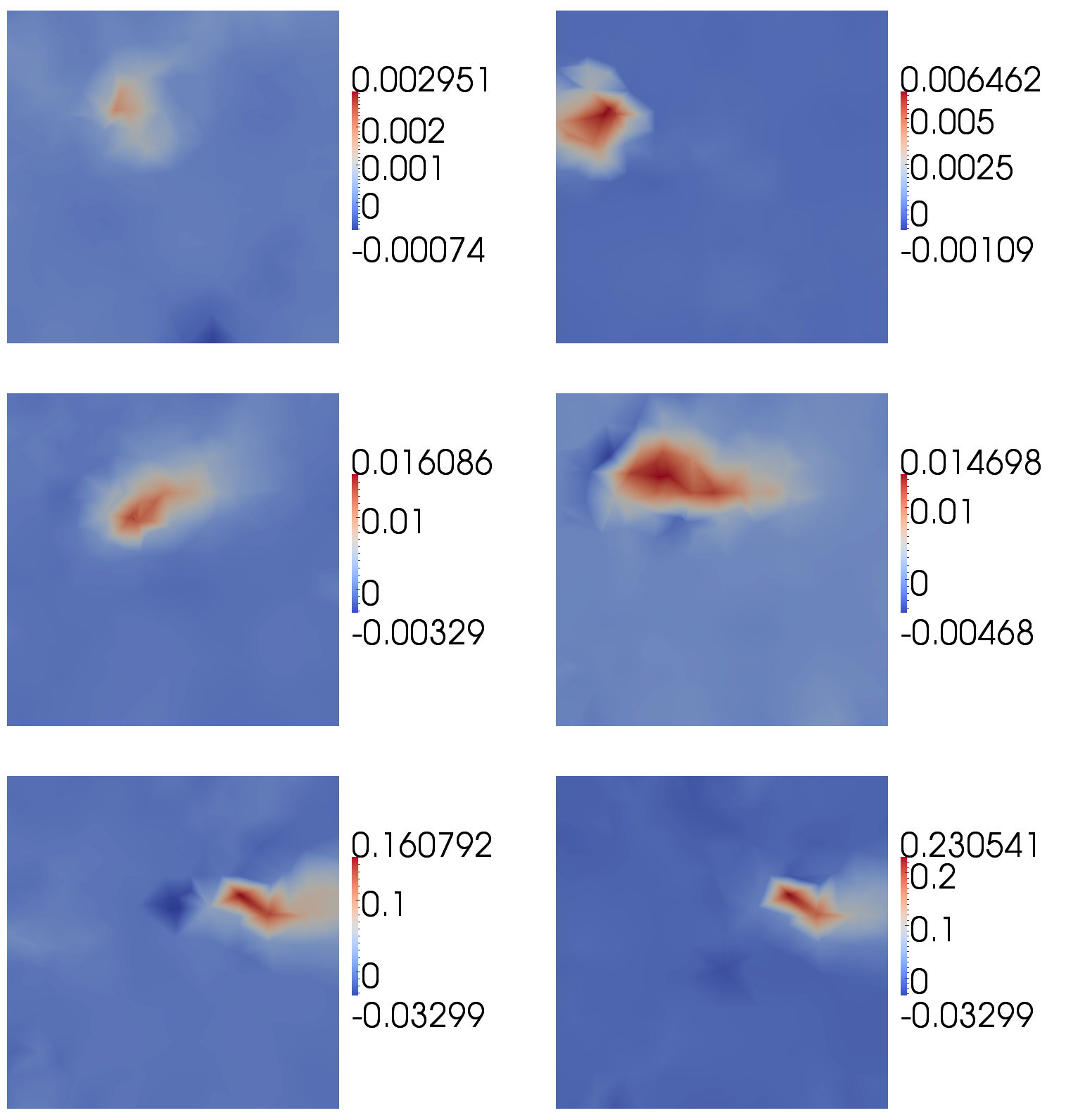
Figure 13: Results are generated by smoothing the perturbations, weighting them with the sensitivity map available at that time, orthogonalising and by using four time windows. Ensemble sizes of 20 (left) and 40 (right) are used. The sensitivity map is shown at times $t=0$ (top), $t=0.175$ (middle) and $t=0.375$ (bottom).

5 Conclusions

We have proposed an optimised method for forming sensitivity maps based on ensembles. We have introduced

• a new goal-based approach, which weights the perturbations with the most up-to-date sensitivities, thereby focusing the perturbations where they will most affect the goal,

• time windows, which enable the perturbations to focus on developing sensitivities specifically for each time window and are thus more accurate,

• re-orthogonalisation of the solution through time, which guarantees that a sensitivity map can be calculated and maximises the information that is obtained from each ensemble member.

The number of ensemble members required to obtain sensitivity maps of a certain precision has been demonstrated to be greatly reduced by combining these techniques. In some of the cases presented here, just 10s of ensemble members are required, making this method extremely appealing when compared to formulating and implementing an adjoint model. Moreover, the presented method is generic and relies solely on perturbations obtained from the forward model. Thus the approach can be applied to forward models of arbitrary complexity, arising from areas such as coupled multi-physics, legacy codes or model chains, without the need to modify the code. There are a number of applications that could benefit greatly from this approach, including the computation of sensitivities for optimisation of sensor placement, optimisation for design or control, goal-based mesh adaptivity, assessment of goals (e.g. hazard assessment and mitigation in the natural environment), determining the worth of current data and data assimilation.

References

- AMCG [2010] AMCG, July 2010. A User’s Guide for the Fluidity Model. Applied Modelling and Computation Group – AMCG.
- Ancell and Hakim [2007] Ancell, B., Hakim, G. K., 2007. Comparing Adjoint- and Ensemble-Sensitivity Analysis with Applications to Observation Targeting. Mon. Weather Rev. 135, 4117–4134.
- Attia [2016] Attia, A., 2016. Advanced Sampling Methods for Solving Large-Scale Inverse Problems. Ph.D. thesis, Department of Computer Science, Virginia Polytechnic Institute and State University.
- Blum et al. [2009] Blum, J., Le Dimet, F.-X., Navon, I. M., 2009. Data Assimilation for Geophysical Fluids. In: Temam, R. M., Tribbia, J. J. (Eds.), Special Volume: Computational Methods for the Atmosphere and the Oceans. Vol. 14 of Handbook of Numerical Analysis. Elsevier, pp. 385–441.
- Brooks and Corey [1964] Brooks, R. H., Corey, A. T., 1964. Hydraulic properties of porous media. In: Hydrology Papers.
- Cacuci [2015] Cacuci, D. G., 2015. Second-order adjoint sensitivity analysis methodology (2nd-ASAM) for computing exactly and efficiently first- and second-order sensitivities in large-scale linear systems: I. Computational methodology. J. Comput. Phys 284, 687–699.
- Cacuci et al. [2012] Cacuci, D. G., Badea, C. M., Badea, A. M., 2012. Best-estimate predictions and model calibration for reactor thermal hydraulics. Nucl. Sci. Eng 172, 1–19.
- Cacuci et al. [2005] Cacuci, D. G., Ionescu-Bujor, M., Navon, I. M., 2005. Sensitivity and Uncertainty Analysis, Volume II: Applications to Large-Scale Systems. CRC Press.
- Cacuci et al. [2013] Cacuci, D. G., Navon, I. M., Ionescu-Bujor, M., 2013. Computational Methods for Data Evaluation and Assimilation. Chapman & Hall.
- Che et al. [2014] Che, Z., Fang, F., Percival, J., Pain, C. C., Matar, O., Navon, I. M., 2014. An ensemble method for sensor optimisation applied to falling liquid films. Int. J. Multiphas. Flow 67, 153–161.
- Daescu and Navon [2004] Daescu, D. N., Navon, I. M., 2004. Adaptive observations in the context of 4D-Var data assimilation. Meteorol. Atmos. Phys 85 (4), 205–226.
- Fang et al. [2011] Fang, F., Pain, C. C., Navon, I. M., Gorman, G. J., Piggott, M. D., Allison, P. A., 2011. The independent set perturbation adjoint method: A new method of differentiating mesh-based fluids models. Int. J. Numer. Meth. Fl. 66 (8), 976–999.
- Gomes et al. [2017] Gomes, J. L. M. A., Pavlidis, D., Salinas, P., Xie, Z., Percival, J. R., Melnikova, Y., Pain, C. C., Jackson, M. D., 2017. A force-balanced control volume finite element method for multiphase porous media flow modelling. Int. J. Numer. Meth. Fl. 83, 431–445.
- Grimit and Mass [2007] Grimit, E. P., Mass, C. F., 2007. Measuring the Ensemble Spread-Error Relationship with a Probabilistic Approach: Stochastic Ensemble Results. Mon. Weather Rev. 135, 203–221.
- Hossen et al. [2012] Hossen, M. J., Navon, I. M., Daescu, D. N., 2012. Effect of random perturbations on adaptive observation techniques. Int. J. Numer. Meth. Fl. 69 (1), 110–123.
- Ionescu-Bujor and Cacuci [2004] Ionescu-Bujor, M., Cacuci, D. G., 2004. A Comparative Review of Sensitivity and Uncertainty Analysis of Large-Scale Systems-I: Deterministic Methods. Nuclear Science and Engineering 147 (3), 189–203.
- Jackson et al. [2015] Jackson, M. D., Percival, J. R., Mostaghimi, P., Tollit, B. S., D. Pavlidis, C. C. P., Gomes, J. L. M. A., El-Sheikh, A. H., P. Salinas, A. H. M., Blunt, M. J., 2015. Reservoir modeling for flow simulation by use of surfaces, adaptive unstructured meshes, and an overlapping-control-volume finite-element method. SPE Reservoir Evaluation and Engineering 18.
- Jain et al. [2018] Jain, P. K., Mandli, K., Hoteit, I., Knio, O., Dawson, C., 2018. Dynamically adaptive data-driven simulation of extreme hydrological flows. Ocean Model. 122, 85–103.
- Jaure et al. [2014] Jaure, S., Moncorge, A., de Loubens, R., 2014. Reservoir Simulation Prototyping Platform for High Performance Computing. In: SPE Large Scale Computing and Big Data Challenges in Reservoir Simulation Conference and Exhibition.
- Jenny et al. [2009] Jenny, P., Tchelepi, H. A., Lee, S. H., 2009. Unconditionally convergent nonlinear solver for hyperbolic conservation laws with S-shaped flux functions. J. Comput. Phys 228, 7497–7512.
- Keller et al. [2010] Keller, J. D., Hense, A., Kornblueh, L., Rhodin, A., 2010. On the Orthogonalization of Bred Vectors. Weather Forecast. 25, 1219–1234.
- Le Dimet et al. [2002] Le Dimet, F.-X., Navon, I. M., Daescu, D. N., 2002. Second-Order Information in Data Assimilation. Mon. Weather Rev. 130 (3), 629–648.
- Leonard [1991] Leonard, B. P., 1991. The ULTIMATE conservative difference scheme applied to unsteady one-dimensional advection. Comput Method Appl. M. 88, 17–74.
- Leroux et al. [2018] Leroux, R., Chatellier, L., David, L., 2018. Time-resolved flow reconstruction with indirect measurements using regression models and Kalman filtered POD ROM. Exp. Fluids 59, 1–27.
- Leutbecher and Palmer [2008] Leutbecher, M., Palmer, T. N., 2008. Ensemble forecasting. J. Comput. Phys 227 (7), 3515–3539.
- Li and Xiu [2009] Li, J., Xiu, D., 2009. A generalized polynomial chaos based ensemble Kalman filter with high accuracy. J. Comput. Phys 228 (15), 5454–5469.
- Liu and Kalnay [2008] Liu, J., Kalnay, E., 2008. Estimating observation impact without adjoint model in an ensemble Kalman filter. Q. J. Roy. Meteor. Soc. 134 (634), 1327–1335.
- Maday and Taddei [2017] Maday, Y., Taddei, T., 2017. Adaptive PBDW approach to state estimation: noisy observations; user-defined update spaces. ArXiv e-prints.
- Meldi and Poux [2017] Meldi, M., Poux, A., 2017. A reduced order model based on Kalman filtering for sequential data assimilation of turbulent flows. J. Comput. Phys 347, 207–234.
- Merton et al. [2013] Merton, S. R., Buchan, A. G., Pain, C. C., Smedley-Stevenson, R. P., 2013. An adjoint-based method for improving computational estimates of a functional obtained from the solution of the Boltzmann Transport Equation. Ann. Nucl. Energy 54, 1–10.
- Merton et al. [2014] Merton, S. R., Smedley-Stevenson, R. P., Pain, C. C., Buchan, A. G., 2014. Adjoint eigenvalue correction for elliptic and hyperbolic neutron transport problems. Prog. Nucl. Energ. 76, 1–16.
- Nerger et al. [2014] Nerger, L., Schulte, S., Bunse-Gerstner, A., 2014. On the influence of model nonlinearity and localization on ensemble Kalman smoothing. Q. J. Roy. Meteor. Soc. 140, 2249–2259.
- Norwood [2015] Norwood, A., 2015. Bred vectors, singular vectors, and Lyapunov vectors in simple and complex models. Ph.D. thesis, University of Maryland.
- Pain et al. [2001] Pain, C. C., Umpleby, A. P., de Oliveira, C. R. E., Goddard, A. J. H., 2001. Tetrahedral mesh optimisation and adaptivity for steady-state and transient finite element calculations. Comput Method Appl. M. 190 (29), 3771–3796.
- Pierce and Giles [2000] Pierce, N. A., Giles, M. B., 2000. Adjoint Recovery of Superconvergent Functionals from PDE Approximations. SIAM Review 42 (2), 247–264.
- Power et al. [2006] Power, P. W., Piggott, M. D., Fang, F., Gorman, G. J., Pain, C. C., Marshall, D. P., Goddard, A. J. H., Navon, I. M., 2006. Adjoint goal-based error norms for adaptive mesh ocean modelling. Ocean Model. 15 (1), 3–38.
- Salinas et al. [2017] Salinas, P., Pavlidis, D., Xie, Z., Jacquemyn, C., Melnikova, Y., Pain, C. C., Jackson, M. D., 2017. Improving the robustness of the control volume finite element method with application to multiphase porous media flow. Int. J. Numer. Meth. Fl. 85, 235–246.
- Shah [2017] Shah, A. J., 2017. Methods for Data Assimilation for the Purpose of Forecasting in the Gulf of Cambay (Khambhat). IJSRSET 3, 224–228.
- Shapiro [1970] Shapiro, R., 1970. Smoothing, Filtering and Boundary Effects. Rev. Geophys. Space Phys 8, 359–387.
- Sun and Mu [2017] Sun, G., Mu, M., 2017. A new approach to identify the sensitivity and importance of physical parameters combination within numerical models using the Lund–Potsdam–Jena (LPJ) model as an example. Theor. Appl. Climatol. 128, 587–601.
- Szunyogh et al. [1997] Szunyogh, I., Kalnay, E., Toth, Z., 1997. A comparison of Lyapunov and optimal vectors in a low-resolution GCM. Tellus A 49 (2), 200–227.
- Toth and Kalnay [1993] Toth, Z., Kalnay, E., 1993. Ensemble Forecasting at NMC: The Generation of Perturbations. B. Am. Meteorol. Soc. 74 (12), 2317–2330.
- Toth and Kalnay [1997] Toth, Z., Kalnay, E., 1997. Ensemble forecasting at NCEP and the breeding method. Mon. Weather Rev. 125 (12), 3297–3319.
- Wang et al. [1992] Wang, Z., Navon, I. M., Le Dimet, F.-X., Zou, X., 1992. The second order adjoint analysis: Theory and applications. Meteorol. Atmos. Phys 50 (1), 3–20.
- Wolfe and Samelson [2007] Wolfe, C. L., Samelson, R. M., 2007. An efficient method for recovering Lyapunov vectors from singular vectors. Tellus A 59 (3), 355–366.
- Xie et al. [2016] Xie, Z., Pavlidis, D., Salinas, P., Percival, J. R., Pain, C. C., Matar, O. K., 2016. A balanced-force control volume finite element method for interfacial flows with surface tension using adaptive anisotropic unstructured meshes. Comput. Fluids 138, 38–50.
- Zupanski [2005] Zupanski, M., 2005. Maximum Likelihood Ensemble Filter: Theoretical Aspects. Mon. Weather Rev. 133 (6), 1710–1726.
- Zupanski et al. [2006] Zupanski, M., Fletcher, S. J., Navon, I. M., Uzunoglu, B., Heikes, R. P., Randall, D. A., Ringler, T. D., Daescu, D., 2006. Initiation of ensemble data assimilation. Tellus A 58 (2), 159–170.