Exotic Multifractal Conductance Fluctuations in Graphene

Abstract

In quantum systems, signatures of multifractality are rare. They have been found only in the multiscaling of eigenfunctions at critical points. Here we demonstrate multifractality in the magnetic-field-induced universal conductance fluctuations of the conductance in a quantum condensed-matter system, namely, high-mobility single-layer graphene field-effect transistors. This multifractality decreases as the temperature increases or as doping moves the system away from the Dirac point. Our measurements and analysis present evidence for an incipient Anderson-localization near the Dirac point as the most plausible cause for this multifractality. Our experiments suggest that multifractality in the scaling behaviour of local eigenfunctions are reflected in macroscopic transport coefficients. We conjecture that an incipient Anderson-localization transition may be the origin of this multifractality. It is possible that multifractality is ubiquitous in transport properties of low-dimensional systems. Indeed, our work suggests that we should look for multifractality in transport in other low-dimensional quantum condensed-matter systems.

1 Introduction

One of the unsolved problems in single-layer graphene (SLG) is the nature of the electronic wave-function near the charge-neutrality (Dirac) point. In principle, the charge-carrier density of SLG should be continuously tunable, down to zero, leading to the largely unexplored regime of extremely weak interactions in a low-carrier-density system. The interaction parameter $r_{\mathrm{s}}$, which parametrizes the ratio of the average inter-electron Coulomb interaction energy to the Fermi energy, turns out to be independent of charge-carrier density in the case of SLG where $r_{\mathrm{s}}=e^{2}/(\kappa\hbar v_{\mathrm{F}})$. Here, $\kappa$ is the dielectric constant of the surrounding medium and $v_{\mathrm{F}}$ is the Fermi velocity. In the case of SLG on an SiO₂ substrate, $r_{\mathrm{s}}$ = 0.8. Thus SLG is a very weakly interacting system, when compared to other conventional two-dimensional systems such as GaAs/AlGaAs and Si inversion layers, where the values of $r_{\mathrm{s}}$ are typically much higher. A naïve application of the scaling theory to such a system in this regime would predict Anderson localization— a disorder-driven quantum phase transition, leading to a complete localization of the charge-carriers, and thence, to an insulator Evers and Mirlin (2008); Ludwig et al. (1994); Cheianov and Falko (2006); Aleiner and Efetov (2006); Katsnelson et al. (2006). Indeed, theoretical calculations for graphene indicate that intervalley scattering can lead to changes in the local and averaged electronic density of states (DOS) with the creation of localized states Pereira et al. (2006); Samaddar et al. (2016). For example, graphene-terminated SiC (0001) surfaces undergo an Anderson-localization transition upon dosing with small amounts of atomic hydrogen Bostwick et al. (2009). This intervalley-scattering-induced localization is most effective near the Dirac point, where the screening of the impurity scatterers is negligible Samaddar et al. (2016). Experiments, however, find the appearance of a minimum conductance value at the Dirac point with $\sigma_{\textrm{min}}\approx 2e^{2}/\pi\hbar$, instead of a diverging resistance which is the hallmark of a truly localized state; notable exceptions being carrier localization Jung et al. (2011) and an Anderson-localization transition in bi-layer graphene heterostructures Ponomarenko et al. (2011).

By studying the scaling behaviour of the universal conductance fluctuations (UCF), we look for signs of charge-carrier localization near the Dirac point in ultra-high mobility SLG and uncover, as a result, an exotic multifractal behaviour in the UCF. Multifractality, characterized by an infinite number of scaling exponents, is ubiquitous in classical systems. Since the pioneering work of Mandelbrot Mandelbrot (1982), the detection and analysis of multifractal scaling in such systems have enhanced our understanding of several complex phenomena, e.g., the dynamics of the human heart-beat Ivanov et al. (1999), the form of critical wave-functions at the Anderson-localization transition Evers and Mirlin (2008), the time series of the Sun’s magnetic field Lawrence et al. (1993), in medical-signal analysis (for instance, in pattern recognition, texture analysis and segmentation) Oudjemia et al. (2013), fully-developed turbulence and in a variety of chaotic systems Frisch (1995); Benzi et al. (1984). In condensed-matter systems, signatures of multifractality are usually sought in the scaling of eigenfunctions at critical points Castellani and Peliti (1986); Janssen (1998); Mirlin (2000); Grussbach and Schreiber (1995); Burmistrov et al. (2015, 2013); Gruzberg et al. (2013); Barrios-Vargas and Naumis (2014). Despite compelling theoretical predictions Facchini et al. (2007); Monthus and Garel (2009); Rammal et al. (1985); Roux et al. (1991); Brandes et al. (1994); Polyakov (1998), there are no reports of the successful observation of multifractality in transport coefficients.

Simple fractal conductance fluctuations, on the other hand, have been observed in several condensed-matter systems Hegger et al. (1996); Micolich et al. (2001); Sachrajda et al. (1998); Ketzmerick (1996); Hegger et al. (1996); Micolich et al. (2001); Ujiie et al. (2008). These arise through semi-classical electron-wave interference processes whenever a system has mixed chaotic-regular dynamics Meiss and Ott (1986); Geisel et al. (1987); Ketzmerick (1996); Hegger et al. (1996). In all these systems, a primary prerequisite for the observation of fractal transport is that the electron dynamics be amenable to semi-classical analysis - the fractal nature of conductance fluctuations seen in these systems disappears as the system is driven deep into the quantum limit. For such a mixed-phase semi-classical system, the graph of conductance ($G$) versus an externally applied magnetic field ($B$) has the same statistical properties as a Gaussian random process with increments of mean zero and variance $(\Delta B)^{\gamma}$. These processes are known as fractional Brownian motion and have the property that their graph is a fractal of dimension $D_{\mathrm{F}}=2-\frac{\gamma}{2}$  Hegger et al. (1996); Ketzmerick (1996), with $1\leq D_{\mathrm{F}}\leq 2$.

A semi-classical description, however, breaks down in the case of materials where the charge-carriers obey a Dirac dispersion relation, e.g., in graphene and topological insulators. In this report, we ask: can we find signatures of multifractality in a quantum system through transport measurements, specifically through the statistical properties of the graph of conductance fluctuations versus an external parameter like the magnetic field? We address this question by studying in detail the statistics of conductance fluctuations in high-mobility SLG-FET devices as a function of the perpendicular magnetic field over a wide range of temperature and doping levels. We report, for the first time, the occurrence of multifractality in the UCF in high mobility graphene devices deep in the quantum limit. Our measurements and analysis suggest at an incipient Anderson localization transition in graphene near the Dirac point.

2 Results

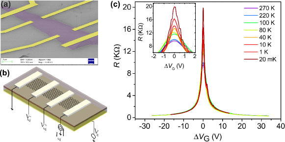
Figure 1: Device structure and characteristics. (a) False-colour SEM image and (b) schematic device configuration of our SLG-FET. The scale-bar in (a) is 2 $\mu m$. (c) Plot of $R$ versus $\Delta V_{\mathrm{G}}$, measured at different temperatures. The values of the temperatures at which the data were collected are mentioned in the legend. In the inset, we plot the same data, zoomed in near the Dirac point ($|\Delta V_{\mathrm{G}}|\leq 2$ V).

Measurement of Universal Conductance Fluctuations.

SLG-FET devices with mobilities in the range $[20,000-30,000]$ cm²V^-1s^-1 were fabricated on SiO₂ substrates by mechanical exfoliation from natural graphite, followed by conventional, electron-beam lithography Novoselov et al. (2005)[Figure 1 (a-b)]. We begin with the dependence of the resistance ($R$) on the gate voltage ($V_{\mathrm{G}}$), for the device G28M6. In Figure 1(c) we show plots of $R$ versus $\Delta V_{\mathrm{G}}=V_{\mathrm{G}}-V_{\mathrm{D}}$, where $V_{\mathrm{D}}$ is the Dirac point, measured at different temperatures ($T$). The high mobility and the position of the charge-neutrality point very close to $V_{\mathrm{G}}=0$ V attests to the high quality of the devices. We measured the magnetoconductance ($G$) as a function of the magnetic field $(\textbf{B}=(0,0,B))$, applied perpendicular to the plane of the device , in the range $-0.2$ T $\leq$ $B$ $\leq$ $0.2$ T. The presence of UCF was confirmed by the appearance of reproducible, non-periodic, but magnetic-field-symmetric, oscillations in $G$. The measurements were performed on multiple devices, over a wide range of $V_{\mathrm{G}}$ and $T$ . We find our UCF data to be in excellent agreement with previous studies of magnetoresistance and conductance fluctuations in single-layer graphene Chen et al. (2010); Berger et al. (2006); Bohra et al. (2012); Tikhonenko et al. (2008); Horsell et al. (2009). Figure 2(a) shows illustrative plots of $G(B)$ with the Fermi energy ($E_{\mathrm{F}}$) maintained very close to the Dirac point [$\Delta V_{\mathrm{G}}~{}\simeq 0$] for the device G28M6. The data for other devices are similar and are shown in the Supplementary Figure 1 [see Supplementary Note 1]. At low values of $|B|$, near the minimum of $G$ at $B=0$, weak-localization corrections are visible [Figure 2(a)]. As we move away from $B=0$, the conductance fluctuations become prominent. The amplitudes of the UCF peaks, and the values of the charge-carrier phase-coherence length $L_{\upphi}$, obtained from the variance of the UCF [Figure 2(b)], decrease with increasing temperature because of thermal dephasing [see Supplementary Note 2]. The temperature dependence of the intervalley-scattering length and the intravalley-scattering length, extracted from weak-localization measurements at $T=$20 mK and $\Delta V_{\mathrm{G}}=$0.2 V, are shown in the Supplementary Figure 4 [see Supplementary Note 3]. We find them to be in excellent agreement with previous studies of localization in single-layer graphene Gorbachev et al. (2007); Tikhonenko et al. (2008). We also observe an increase in $L_{\upphi}$ with increasing $|\Delta V_{\mathrm{G}}|=|V_{\mathrm{G}}-V_{\mathrm{D}}|$ [Figure 2(c)], which we attribute to the increase in the screening of impurities by charge carriers Chen et al. (2010). We note an apparant saturation of $L_{\upphi}$ below a temperature of $\simeq 100$ mK. The saturation of the phase-coherence length ($L_{\upphi}$) with decreasing temperature is an issue that has been at the forefront of research in several other semiconducting materials including doped Si Mohanty and Webb (2003, 1997); Pierre et al. (2003). There are many effects, e.g. the presence of magnetic impurities Pierre et al. (2003) or finite size, which can lead to a saturation of $L_{\upphi}$. We note here that a decoupling of the electron and lattice temperature leading to a saturation of the $L_{\upphi}$ is also possible. However, the data shown in Figure 1(c) and Figure 2(a) show a continuous evolution of both the conductance and conductance fluctuations down to 20 mK. This rules out any saturation of the electron temperature down to 20 mK, and hence, the observed saturation of $L_{\upphi}$ below a certian temperature is not an experimental artifact [see Supplementary Note 3]. In a separate set of measurements, we obtain the magnitude of the UCF, at a given magnetic field, by sweeping over $V_{\mathrm{G}}$ and calculating the rms value of the fluctuations. We found that this quantity decreased sharply with increasing magnetic field [see Supplementary Note 4, Supplementary Figure 5] in conformity with theoretical predictions Liu et al. (2016).

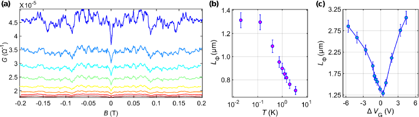
Figure 2: UCF in graphene. (a) Illustrative plots of the magnetoconductance $G$ versus the magnetic field $B$ measured at 0.02 K, 0.05 K, 0.07 5K, 0.10 K, 0.20 K, 0.50 K, 1.00 K, and 2.00 K (from top to bottom - curves for different temperatures have been shifted vertically for clarity). The data shown here are from the device G28M6 measured close to the Dirac point ( $\Delta V_{\mathrm{G}}=0.2$ V). (b) Plot of the phase-coherence length $L_{\upphi}$ versus the temperature $T$ extracted from the UCF measured at $\Delta V_{\mathrm{G}}=0.2$ V. (c) Plot of $L_{\upphi}$ versus $\Delta V_{\mathrm{G}}$, extracted from the UCF measured at $T=$ 20 mK. The error-bars in (b) and (c) represent the standard deviation in $L_{\upphi}$.

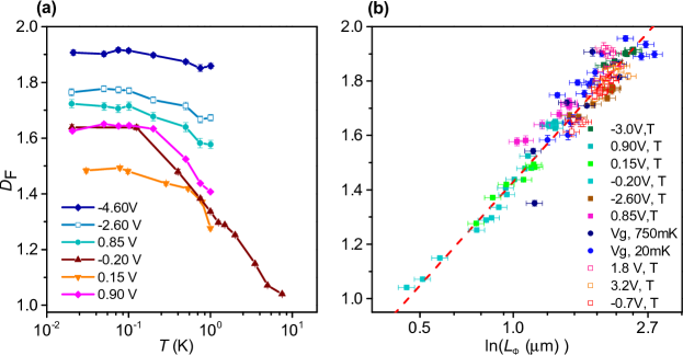
Figure 3: Fractal dimension of UCF in graphene. (a) Plots of the fractal dimension $D_{\mathrm{F}}$ versus the temperature $T$ for different values of $\Delta V_{\mathrm{G}}$. The error-bars represent the standard deviation in $D_{\rm F}$. (b) $D_{\mathrm{F}}$ versus the charge-carrier phase-coherence length $L_{\upphi}$ on a semi-log scale; the data points, with error bars representing standard deviation in $D_{\rm F}$ and $L_{\upphi}$., are from two different devices (filled symbols: G28M6; open symbols: G30M4) and for the following parameter ranges: $20~{}\rm{mK}<$ $T$ $<10~{}\rm{K}$ and $-4.5~{}\rm{V}<\Delta V_{\mathrm{G}}<4.5$ V. The numbers in the legend refer to the ($V_{\mathrm{G}},T$) parameter space. The red curve is $D_{\mathrm{F}}\propto\ln(L_{\upphi})$ (see text).

Analysis of Fractal scaling of the UCF.

UCF represents quantum correction to Drude conductivity arising from the interference of electronic wavefunctions; and it is fingerprint of the disorder configuration in the conducting channel. Besides information about the phase-coherence of the charge carriers, it can also provide crucial insights into the electron dynamics and distribution of eigenstates through a scaling-dimension analysis of the magnetoconductance traces Ketzmerick (1996); Hegger et al. (1996); Micolich et al. (2001). We first compute the simple fractal dimensions $D_{\mathrm{F}}$ of the UCF curves via the Ketzmeric-variance method [Supplementary Note 5]. Figure 3(a) shows plots of $D_{\mathrm{F}}$ versus $T$ for the device G28M6. At very low $T$ and small $|\Delta V_{\mathrm{G}}|$, we find $1<D_{\mathrm{F}}<2$. With increasing temperature, $D_{\mathrm{F}}$ $\to$1 monotonically. In this high-$T$ regime, the thermal-diffusion length $L_{\mathrm{T}}=\sqrt{\hbar D/k_{\mathrm{B}}T}\ll L_{\upphi}$, with $D$ the thermal-diffusion coefficient of the charge carriers; therefore, quasiparticle phase-decoherence, induced by inelastic thermal scattering, suppresses quantum interference. For large $|\Delta V_{\mathrm{G}}|$, the magnitude of the UCF is comparable to, or smaller than the background electrical noise, so $D_{\mathrm{F}}$$\to$$2$, the value for Gaussian white noise. In Figure 3(b), we plot $D_{\mathrm{F}}$ versus $L_{\upphi}$ for two different devices: G28M6 and G30M4; remarkably, all the data points from these two devices cluster in the vicinity of a curve, with $D_{\mathrm{F}}\propto\ln(L_{\upphi})$. In the limits $L_{\upphi}\ll L$, the UCF is non-fractal ($D_{\mathrm{F}}\simeq 1$), where as for large $L_{\upphi}$, the UCF is a fractal, so $1<D_{\mathrm{F}}<2$.

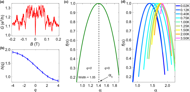
Figure 4: Multifractality of UCF in graphene. (a) A typical plot of the magnetoconductance at $T=20$mK, $\Delta V_{\mathrm{G}}=0.2$ V for our device G28M6. (b) Plot of the generalized Hurst exponent $h(q)$ versus $q$, calculated from the UCF data in (a). A few representative error bars, defining the standard deviation in the data, are shown in the plot. (c) Plot of the multifractal singularity spectrum $f(\alpha)$ versus $\alpha$ that follows from the $h(q)$ versus $q$ data plotted in (b). The dotted vertical line marks the location of the maximum of $f(\alpha)$. (d) Plots illustrating the temperature dependence of $f(\alpha)$ at $\Delta V_{\mathrm{G}}=0.2$ V for the device G28M6.

Analysis of Multifractal scaling of the UCF.

We build upon the predictions of multifractal scaling of conductance fluctuations in quantum systems Facchini et al. (2007) by carrying out a multifractal detrended fluctuation analysis [Supplementary Note 6] of our UCF. The multifractality can be represented in the following two ways: (1) By the generalized Hurst exponent $h(q)$, defined using the order-$q$ moment of the UCF as $\langle{\rm rms}[\Delta G(\Delta B)]^{q}\rangle^{1/q}\sim[\Delta B]^{h(q)}$, and (2) by the multifractal spectrum $f(\alpha)$, obtained from the Legendre transform of $h(q)$. For a monofractal function, $h(q)$ has a single, $q$-independent value. For each one of our UCF plots, we obtain $h(q)$ in the range $-4\leq q\leq 4$. In Figure 4(b), we give an illustrative plot of $h(q)$ versus $q$ that we obtain from our magnetoconductance data at 20 mK [Figure 4(a)]; $h(q)$ goes smoothly from $\simeq 1.9$, at $q=-4$, to $\simeq 0.85$, at $q=4$; the corresponding $f(\alpha)$ spectrum is plotted in Figure 4(c). The singularity spectra have a definite maximum value of 1 (which is the dimension of the support graph). The width of the multifractal spectrum is defined as $\Delta\alpha\equiv$ $h(q)_{\rm max}$ -$h(q)_{\rm min}$. The wide range of $h(q)$, or, equivalently, the wide spectrum ($\Delta\alpha$=1.05) quantifies the multifractality of the UCF. This is the first observation of multifractality of a conductance in any quantum-condensed-matter system and is the central result of our work.

We note that there are two distinct properties of UCF that can give rise to its multifractal behaviour Gu and Zhou (2010); Zhou (2009): (i) a fat-tailed, non-Gaussian distribution of the UCF differences (as a function of $\delta B$) or (ii) long-range, in the magnetic field $B$, correlations of the fluctuations of $\delta g(B)$. We have verified that the distribution of our measured $\delta g(B)$ is not log-normal. Having ruled out (i), we now give a convenient test for (ii): we check for multifractality in a data set obtained from a random shuffling [see Supplementary Note 7] of the original sequence of $\delta g(B)$. If the long-range correlations (ii) exist, then signatures of multifractality must be absent in the reshuffled data. Indeed, in our experimental data, we observe a near-complete suppression of multifractality in the shuffled data set with $h_{\rm shuf}(q)\simeq 0.5$ for all values of $q$ and $\Delta\alpha=$0.05 [Supplmentary Figure 9]. Hence it is reasonable to infer that the multifractality in our UCF can be traced back to long-ranged correlations, that are otherwise difficult to measure.

Figure 4(d) shows plots of $f(\alpha)$ for different values of $T$ and $\Delta V_{G}=0.2$V. The symmetry of $f(\alpha)$ about $\alpha_{0}$ [Figure 4(c)] reflects the distribution of fluctuations, about the mean of the UCF. The large-fluctuation (small-fluctuation) segments contribute predominantly to the $q>0$ ($q<0$) part of $h(q)$. The $q>0$ ($q<0$) part of $h(q)$ maps onto the $\alpha<\alpha_{0}$ ( $\alpha>\alpha_{0}$) region of $f(\alpha)$, which is more-or-less symmetric about $\alpha_{0}$ at low $T$ [Figure 4(d)]. As we increase $T$, this symmetry is lost. The magnitude of the skewness $\langle[\delta\alpha]^{3}\rangle/\langle[\delta\alpha]^{2}\rangle^{3/2}$, where $\delta\alpha=(\alpha-\alpha_{0})$, increases with $T$. Therefore, as $T$ increases, large-amplitude conductance fluctuations become rarer than small-amplitude fluctuations. This is consistent with our plots of the UCF [Figure 2(a)].

3 Discussion

A naïve characterization of the fractal property of a curve, say by the measurement of one fractal dimension, does not rule out multifractality of this curve, which requires the calculation of an infinite number of dimensions Grassberger and Procaccia (1983) (related to $h(q)$). One dimension suffices for monofractal scaling (as, e.g., in the scaling of velocity structure functions in the inverse-cascade region of forced, two-dimensional fluid turbulence Kellay and Goldburg (2002); Boffetta and Ecke (2012)). Our measurements of the UCF in single-layer graphene show that it is multifractal only if (i) the temperature is low and (ii) $\Delta V_{\mathrm{G}}\simeq 0$. If either one of these conditions is not met, the plot of $\delta g$ versus $B$ is a monofractal [see Supplementary Note 8]; at sufficiently large $T$, $D_{\mathrm{F}}\to$1 and the plots are non-fractal.

What can be the possible origin of our multifractal UCF? We list three potential causes: (1) scarring of wave functions (e.g., because of classically-chaotic billiards Heller (1984)); (2) quasi-periodicity in the Hamiltonian induced by a magnetic field Harper (1955); Hofstadter (1976); Ostlund et al. (1983) and its analogue for graphene Sena et al. (2010); (3) Anderson-localization-induced multifractality Evers and Mirlin (2008). We critically examine each one of these possibilities below and conclude that our results are most compatible with the last of these mechanisms.

While describing a quantum system, whose classical analogue is chaotic, one encounters scarred wavefunctions, whose intensity is enhanced along unstable, periodic orbits of the classical system. This non-uniform distribution of intensity of wavefunctions results from quasiparticle interference. Quantum scars can lead to pointer states Zurek (1981) with long trapping times, and, consequently, to large conductance fluctuations. Relativistic quantum scars have been predicted theoretically in geometrically confined graphene stadia, which exhibit classical chaos Huang et al. (2009). However, our devices are not shaped like billiards that are classically chaotic; and the charge carriers are not in the ballistic regime. Therefore, quantum scars cannot be the underlying cause for our multifractal UCF.

Fractal energy spectra can arise in tight-binding problems with an external magnetic field, which can be mapped onto Schrödinger problems with quasiperiodic potentials Harper (1955); Hofstadter (1976); Ostlund et al. (1983); Ostlund and Pandit (1984). It has been argued Sena et al. (2010), therefore, that a fractal conductance can also arise, via Hofstadter-butterfly-type spectra, in Dirac systems at sufficiently high magnetic fields $B_{\mathrm{H}}\simeq\phi_{0}/A_{0}$ ($\simeq 10^{5}$ T for our samples), where $\phi_{0}=2\pi\hbar/e$ is the flux quantum and $A_{0}$ is the unit-cell area. Our measurements use very-low-magnitude magnetic fields ($\lesssim 0.2$ T); this rules out a quasi-periodicity-induced multifractal UCF.

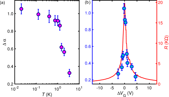
Figure 5: Width of the multifractal spectrum. (a) Blue filled circles (left axis) show the dependence of the width of the multifractal spectrum, $\Delta\alpha$ on $\Delta V_{\mathrm{G}}$; the data were obtained at 20 mK. The red line shows the dependence of $R$ on $V_{\mathrm{G}}$, measured at 20 mK (right axis). It is clear from the plot that $\Delta\alpha$ is large only over a narrow range of gate voltage around $\Delta V_{\mathrm{G}}=0$ V, and sharply decreases as the system is driven away from the Dirac point. (b) Dependence of the width $\Delta\alpha$ on temperature, at $\Delta V_{\mathrm{G}}=0.2$ V; the data were obtained from the UCF plots shown in Figure 2(a). The error-bars in (a) and (b) represent the standard deviation in $\Delta\alpha$.

The most compelling explanation of the multifractal UCF we observe in our SLG samples is an incipient Anderson localization near the charge-neutrality point. Multifractality of the local amplitudes of critical eigenstates near Anderson localization has been studied, theoretically, in several quantum-condensed-matter systems Mirlin (2000); Burmistrov et al. (2013); Gruzberg et al. (2013); Barrios-Vargas and Naumis (2014). The multifractality of the eigenstates near the critical point directly affects the two-particle correlation function through the generalized diffusion coefficient Brandes et al. (1996); Harris and Aharony (1987), which, in turn, affects the local current fluctuations in the system via the Kubo formula. It is not obvious that this must be reflected in the (macroscopic) conductance, or its moments; however, it is plausible that near the critical point, the UCF may inherit multifractal behaviour from its counterpart in the eigenfunctions Benenti et al. (2001). Indeed, there are several theoretical predictions of multifractality in transport coefficients including conductance jumps near the percolation threshold in random-resistor networks Rammal et al. (1985); Roux et al. (1991), conductance fluctuations in quantum-Hall transitions Brandes et al. (1994), and the temperature dependence of the peak height of the conductance at the Anderson-localization transition Polyakov (1998).

Spectroscopic studies on single-layer on-substrate graphene devices have revealed that the local potential fluctuations in this system are strongest when $E_{F}$ is close to the Dirac point Samaddar et al. (2016); Jung et al. (2011). This leads to electronic states that are quasi-localized  Ugeda et al. (2010); Shytov et al. (2007); Das Sarma et al. (2011). Such quasi-localized states have a high inverse participation ratio Pereira et al. (2006) that can lead to the multifractality seen in our experiments. If this is true, then the multifractality in the UCF should be largest near the Dirac point; and then fall off on either side of it. In Figure 5 we show the dependence of $\Delta\alpha$ on $T$ and $\Delta V_{\mathrm{G}}$ for the device G28M6 [data obtained for other devices are qualitatively similar]. We observe that $\Delta\alpha$ is indeed largest near $\Delta V_{\mathrm{G}}=0$ and at low $T$, where the conductance of the device is of the order of $e^{2}/h$, and it sharply decreases as either $T$ or the magnitude of $\Delta V_{\mathrm{G}}$ increases. Similarly, as $T$ is increased, thermal scattering increases quasiparticle dephasing, and eventually at high $T$, when $L_{\upphi}\sim L_{\mathrm{T}}\ll L$, quantum-interference effects are masked. From our observation that a large multifractality arises only when quantum-interference-induced charge-carrier localization is significant, we propose that an incipient Anderson localization near the Dirac point is the most plausible origin of multifractal UCF in SLG.

This interpretation of the multifractality of the UCF in single-layer graphene devices is based on previous theoretical predictions and analysis. We summarize our argument below:

Conductance fluctuations, as a function of the magnetic field, have been shown to have a fractional fractal dimensions in some simple, one-dimensional, quantum systems, e.g., the kicked rotor Benenti et al. (2001); Casati et al. (2000). In these systems, such a fractional fractal dimension arises if one of the following conditions holds: (1) The PDF $P(t)$, of the charge-carrier survival time $t$, has a power-law form $P(t)\propto t^{-\gamma}$ at large $t$ (as opposed to an exponential decay); (2) the energy correlation $C(\Delta E)$ of elements of the S-matrix exhibit power laws (i.e., $C(\Delta E)\propto(\Delta E)^{-\gamma}$) Ketzmerick (1996); Casati et al. (2000); Hegger et al. (1996); Lai et al. (1992). Such survival probabilities are related to the conductance Casati et al. (2000); Benenti et al. (2001); and their multifractal behaviour has been explored Facchini et al. (2007).

At the Anderson-localization transition, it is known that both the probability density function describing the diffusion of a wave-packet and the two-particle correlation function decay algebraically with a fractional power Brandes et al. (1996); Harris and Aharony (1987); Nakayama and Yakubo (2013). Hence, as in the case of the simple quantum systems mentioned above, we may expect multifractal fluctuations of the conductance at the Anderson-localization transition. However, to the best of our knowledge, there are no exact, analytical results that yield a one-to-one correspondence between the multifractality of a critical wavefunction and the multifractality of the magnetoconductance. Thus, we propose that the multifractality of the critical wavefunctions at the Anderson localization is the most plausible cause of the multifractality of the UCF we have observed.

4 Conclusions

In conclusion, we have uncovered and quantified the multifractal structure of mesoscopic conductance fluctuations in single-layer graphene devices. We speculate that our results are indicative of an incipient Anderson localization in this system. In particular, we quantify the multifractality of transport in a quantum condensed-matter system. There may well be multifractality in transport properties in systems other than graphene, and that multifractality is not unique to graphene. Our work provides a natural framework for studying the multifractality of such transport properties.

5 Acknowledgements

We acknowledge discussions with A. D. Mirlin and S. Bhattacharjee. A.B. acknowledges financial support from Nanomission, DST, Govt. of India project SR/NM/NS-35/2012; SERB, DST, Govt. of India and Indo-French Centre for the Promotion of Advanced Recearch (CEFIPRA). K.R.A. thanks CSIR, MHRD, Govt. of India for financial support. S.S.R. acknowledge financial support from the AIRBUS Group Corporate Foundation Chair in Mathematics of Complex Systems established in ICTS-TIFR, the support from DST, Govt. of India, project ECR/2015/000361, and the Indo-French Center for Applied Mathematics (IFCAM). R.P. acknowledges DST, Govt. of India for support. N.P. thanks UGC, Govt. of India for financial support.

6 Author contributions

K.R.A and A.B. designed the experiment, fabricated the devices and carried out the measurements. K.R.A., A.B., N.P. and S.S.R. carried out the data analysis. All authors discussed the results and wrote the paper.

References

Supplementary Information

SUPPLEMENTARY NOTE 1 UCF data

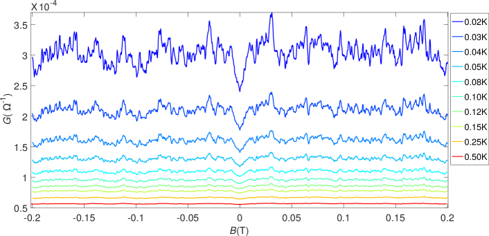
Supplementary Figure 1: Plot of UCF. Illustrative plots of the magnetoconductance ($G$) versus magnetic field ($B$), for our device G30M4, measured at different temperatures, with $\Delta V_{\mathrm{G}}=-0.7$ V. The data have been shifted vertically for clarity.

Supplementary Figure 1 shows plots of the magnetoconductance at different temperatures ($T$), for our device G30M4. The data have been vertically shifted for clarity. The measurements were carried out at a fixed gate voltage $\Delta V_{\mathrm{G}}=-0.7$ V. Each of the magnetoconductance plots show aperiodic oscillations, which are symmetric in magnetic field ($B$). The amplitude of the oscillations gets suppressed with increasing $T$, however, all the oscillation features (peaks and dips in the magnetoconductance) appear at exact same value of $B$. These symmetric and reproducible oscillations are the signatures of UCF.

We first symmetrize each of the the magnetoconductance

$$G_{\rm sym}(B)=\frac{G(B)+G(-B)}{2},$$ (S1)

to remove the anti-symmetric noise contribution from our data. This symmetric component, henceforth referred to as $G(B)$, is used for all our subsequent analysis.

SUPPLEMENTARY NOTE 2 Phase Coherence Length

We estimate the phase-coherence length ($L_{\upphi}$) by two standard methods, other than obtaining from the UCF variance Beenakker and van Houten (1991), which provid, qualitatively, similar result [$L_{\upphi}$ dependence of $D_{\mathrm{F}}$, shown in Fig. 3(b) of the manuscript]. First, we extract $L_{\upphi}$ by fitting the weak-localization peak with the Hikami-Larkin-Nagaoka equation Tikhonenko et al. (2008),

$$\Delta\sigma=\frac{e^{2}}{\pi h}\times\bigg{[}F\bigg{(}\frac{8\pi B}{\Phi_{0}L_{\upphi}^{-2}}\bigg{)}-F\bigg{(}\frac{8\pi B}{\Phi_{0}\big{[}L_{\upphi}^{-2}+2L_{\mathrm{i}}^{-2}\big{]}}\bigg{)}-2F\bigg{(}\frac{8\pi B}{\Phi_{0}\big{[}L_{\upphi}^{-2}+L_{\mathrm{i}}^{-2}+L_{\ast}^{-2}\big{]}}\bigg{)}\bigg{]}$$ (S2)

where $F(z)=\ln z+\psi(0.5+z^{-1})$, and $\psi(x)$ is the digamma function, $L_{\mathrm{i}}$ and $L_{\ast}$ are the characteristic length scale for inter-valley scattering and intra-valley scattering, respectively. The first term in Eqn. S2 gives the weak-localization correction, and the other terms are attributed to weak anti-localization.

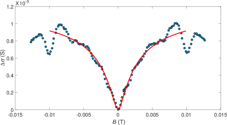
Supplementary Figure 2: Fit with the HLN equation to extract $L_{\upphi}$. A representative plot of $\Delta\sigma$ versus magnetic field $B$ is shown here. The filled circles represent the data points and the red thick line is the fit to the data using Eqn. S2.

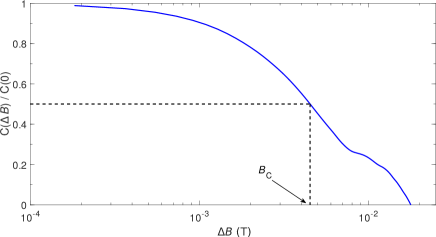
Supplementary Figure 3: $L_{\upphi}$ from autocorrelation of UCF. Plot of normalized autocorrelation $C(\Delta B)/C(0)$ versus $\Delta B$. The correlation field $B_{\mathrm{C}}$, defined as the magnetic field at which the normalized autocorrelation becomes 0.5, is marked with an arrow.

Supplementary Table 1: Comparison of $L_{\upphi}$ extracted via different methods

Method	UCF variance	HLN fit	autocorrelation of UCF
$L_{\upphi}$($\mu$m)	1.20	1.27	0.96

Supplementary Figure 2 shows plots of a typical $\Delta\sigma=\sigma(B)-\sigma(0)$ versus $B$, and the fit to the data with Eqn. S2. The extracted value of $L_{\upphi}$ from the fit is $1.27~{}\mu$m (Supplementary Table 1).

$L_{\upphi}$ was also estimated from the auto-correlation ($C(\Delta B)$) of the UCF Beenakker and van Houten (1991); Horsell et al. (2009). The autocorrelation of the magnetoconductance is defined as

$$C(\Delta B)=\int dBG(B)G(B+\Delta B).$$ (S3)

The correlation magnetic field $B_{\mathrm{C}}$ is then obtained from the autocorrelation $C(\Delta B)$ using the relation,

$$C(B_{\mathrm{C}})=\frac{1}{2}C(0).$$ (S4)

$L_{\upphi}$, is then calculated from $B_{\mathrm{C}}$ using the relation

$$L_{\upphi}=\sqrt{h/eB_{\mathrm{C}}}.$$ (S5)

Supplementary Figure 3 shows plot of normalized autocorrelation $C(\Delta B)/C(0)$ versus $\Delta B$ for the same UCF data [for which the fit with the HLN equation is shown in Supplementary Figure 2].

A comparison of values of $L_{\upphi}$ extracted from a UCF data, measured at $T=0.2$ mK, using the above-mentioned different methods are shown in Supplementary Table 1.

SUPPLEMENTARY NOTE 3 Effect of Temperature on UCF

Plot of the rms value of the magnetoconductance fluctuation ($\delta G_{\rm rms}$) versus $T$ is shown in  Supplementary Figure 4(a). The UCF corresponding to this data were measured at $\Delta V_{\mathrm{G}}=$0.2 V [UCF series shown in Fig. 2(a) of main text]. We observe a strong suppression of the magnetoconductance fluctuations with increasing temperature which is directly attributed to charge carrier dephasing induced by thermal scattering Chen et al. (2010); Berger et al. (2006); Bohra et al. (2012); Tikhonenko et al. (2008); Horsell et al. (2009).

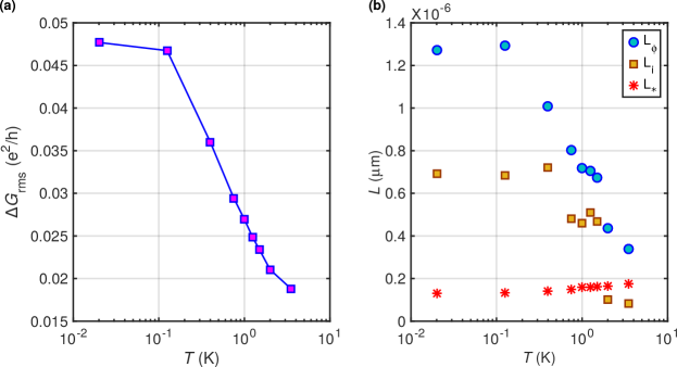
Supplementary Figure 4: Effect of $T$ on UCF. (a) Plot of rms value of UCF, measured at $\Delta V_{G}=$0.2 V, as a function of T. (b) Plot of $L_{\upphi}$ , $L_{\mathrm{i}}$ and $L_{\ast}$ extracted from fitting the magnetoresistance data with the HLN equation (Eqn S2), at $T=$20 mK and $\Delta V_{\mathrm{G}}=$ 0.2 V.

Supplementary Figure 4(b) shows plots of $L_{\upphi}$ (in blue filled circles), $L_{\mathrm{i}}$ (in yellow filled squares) and $L_{\ast}$ (in red asterisk) versus $T$, extracted from fitting the weak localization correction in the magnetoresistance data with the HLN equation (Eqn. S2), at $T=20$ mK and $\Delta V_{\mathrm{G}}=0.2$ V. We find that the goodness of the fit is strongly influenced by the presence of UCF, as was observed by other groups as well Gorbachev et al. (2007); Tikhonenko et al. (2008).

We observe some evidence of a labelling off of $L_{\upphi}(T)$ around 100 mK. This is an issue that has been at the forefront of research in several other semiconducting materials including doped Si Mohanty and Webb (2003, 1997); Pierre et al. (2003). Saturation of $L_{\upphi}(T)$ have been observed in graphene at a much higher temperatures ($\sim 4$ K) and had been argued to arise from finite-size effects Tikhonenko et al. (2008). The presence of disorder also enhances the saturation of $L_{\upphi}$. This is because the presence of disorder leads to the formation of electron-hole puddles, which modify the conducting paths and decrease the effective size of the device Tikhonenko et al. (2008). This, in turn, results in a size-limited saturation of $L_{\upphi}$. Earlier experiments have also shown that, scattering from extremely low concentration of magnetic impurity, even at a level undetectable by other means, can lead to the widely observed saturation of $L_{\upphi}$ (or equivalently, the dephasing time $\tau_{\upphi}$ ) in weakly disordered systems Pierre et al. (2003). Our device has a higher mobility and a longer channel length than in Ref Tikhonenko et al. (2008). Thus we expect the effects of disorder and small channel length, which typically leads to a saturation of $L_{\upphi}$, to be much weaker in our device. Hence, it is reasonable to observe a stronger temperature dependence of $L_{\upphi}$ down to lower temperatures, and a probable saturation only below 0.1 K.

SUPPLEMENTARY NOTE 4 UCF at different magnetic fields

We have also measured UCF at a fixed magnetic field, by varying gate-voltage. We compare the rms value of the magnetoconductance fluctuations ($\delta G_{\rm rms}$) measured in two different ways: (1) at a constant magnetic field by varying gate voltage, and (2) at a constant gate voltage (with $\Delta V_{\mathrm{G}}\sim$ 0) by varying the magnetic field. We observe that the magnitude of the UCF measured during the gate sweep is $\sim$ 1.6 times larger than the UCF measured during the field sweep, which indicates non-ergodicity of UCF Liu et al. (2016).

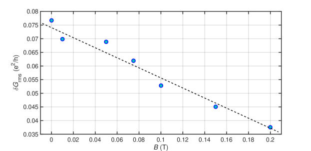
Supplementary Figure 5: UCF amplitude versus B. Typical plot of $\delta G_{\rm rms}$ versus $B$ - the data were acquired by sweeping the gate voltage at a fixed magnetic field. The data were acquired at $T=$20 mK. Blue filled circles represent the data and the dashed line is guide to the eye.

Furthermore, we have carried out UCF measurements by sweeping the gate voltage at different values of the magnetic field in the range of 0 T to 0.2 T. In Supplementary Figure 5, we plot the rms value of conductance fluctuations, $\delta G_{\rm rms}$ versus $B$. We find that $\delta G_{\rm rms}$ decreases with increasing $B$. These observations are in excellent agreement with predictions of behaviour of UCF in the presence of long-range component of random scattering potential Liu et al. (2016).

SUPPLEMENTARY NOTE 5 Calculation of fractal dimensions

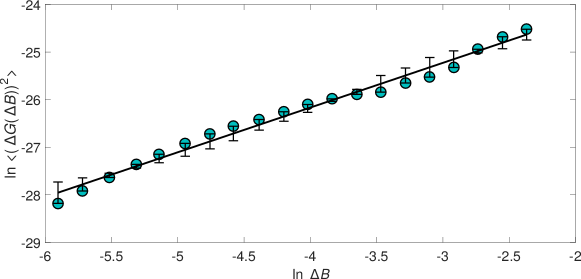
Supplementary Figure 6: Fractal scaling plot. A representative, ln-ln plot of $\langle(\Delta G(\Delta B))^{2}\rangle$ versus $\Delta B$ from a typical UCF. The filled circles are the data from our experiment and the thick black line connecting them is the linear best-fit that yields $D_{\mathrm{F}}\simeq 1.5$. The error-bars represent deviation of the data-points from the best-fit line.

We calculate the fractal dimensions, from our UCF data, in the following way.

We begin by defining and calculating $\delta G(B)$ = $G(B)-\langle G(B)\rangle$, where the angular brackets define the average of over $B$. To calculate the fractal dimension, we begin Ketzmerick (1996) by dividing our UCF data into $N_{s}$ overlapping segments of size $\Delta B$. We then define $\Delta G(\Delta B)\equiv\delta G(B)-\delta G(B+\Delta B)$ from which we calculate $\langle(\Delta G(\Delta B))^{2}\rangle$, where we average over all the $N_{s}$ segments. Thence we evaluate $\langle(\Delta G(\Delta B))^{2}\rangle$ for different values of $\Delta B$, and study the scaling. Typically, $\langle(\Delta G(\Delta B))^{2}\rangle~{}\sim~{}(\Delta B)^{\gamma}$. From fits to log-log plots of $\langle(\Delta G(\Delta B))^{2}\rangle$ versus $\Delta B$ (see Supplementary Figure 6 for a representative example), we obtain from our data the value of $\gamma$, which yields the fractal dimension $D_{\mathrm{F}}$ via $D_{\mathrm{F}}=2-\gamma/2$; for the data shown in Supplementary Figure 6, this yields $D_{\mathrm{F}}\simeq 1.5$.

SUPPLEMENTARY NOTE 6 Calculating multifractal exponents

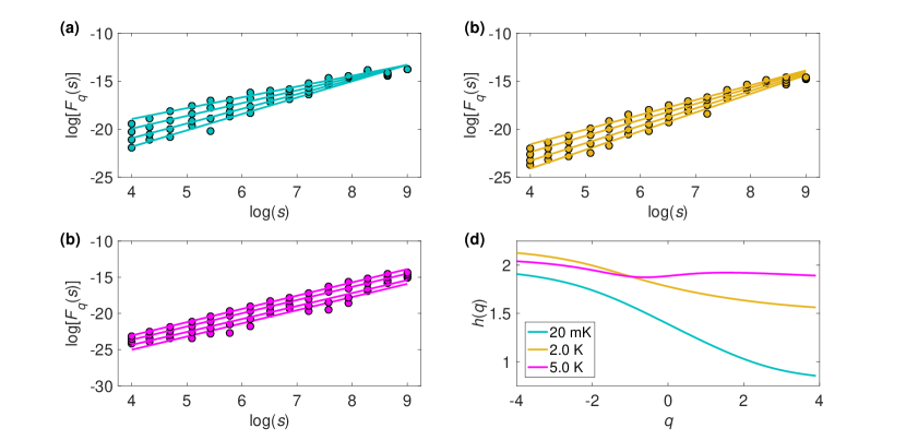
Supplementary Figure 7: Multifractal scaling plot. (a)-(c) Plots of $\log[F_{q}(s)]$ [Eqn. S8] as a function of scale size $\log(s)$ for different orders $q$. The text inside the figures indicate the temperature at which the measurements were made. (d) A plot of the order-$q$ scaling exponent $h(q)$ as a function of $q$; these exponents have been extracted from the plots (a)-(c), as discussed in the text.

We compute the multifractal singularity spectrum form our UCF by using the method of Multifractal Detrended Fluctuation Analysis (MFDFA) Kantelhardt (2012), which we describe below.

We begin by a local detrending of our data. To do this, we choose a segment of the magnetic field $\Delta B$ and then divide the UCF into different overlapping segments. We then fit the different segments of our conductance data ${G}$ with a polynomial $P_{m}$ and remove the local trend:

$$g(i)=G(i)-P_{m}(i).$$ (S6)

It is important to keep the same order $m$ of the polynomial throughout this analysis and for all the segments. Alternatively, we can divide the conductance data ${G}$, with $N$ data points, into $N_{s}$ segments: $N_{s}=int(N/s)$, with $s$ points in each segment. In our analysis, the detrending is done with a polynomial of order 1.

Next, we evaluate the root-mean-square (rms) fluctuations and the order-$q$ moment of these fluctuation via

$$g_{\rm rms}=\left(\frac{1}{s}\sum_{i=1}^{s}g(i)^{2}\right)^{1/2}.$$ (S7)

We then define

$$F_{q}(s)=\left(\frac{1}{N_{s}}\sum_{j=i}^{N_{s}}g_{\rm rms}(j)^{q}\right)^{1/q}.$$ (S8)

In Supplementary Figure 7(a-c) we show representative (log-log) plots of $F_{q}$ versus $s$ for three different temperatures and for different values of $q$. From such plots it is possible to calculate the generalized order-$q$ scaling exponent through the scaling relation

$$F_{q}(s)\sim s^{H(q)}.$$ (S9)

We calculate the order-$q$ scaling exponent $H(q)$ for different values of $q$ and at different temperatures. In Supplementary Figure 7(d) we show a representative plot of $H(q)$ versus $q$ from data at the three temperatures shown in Supplementary Figure 7(a-c).

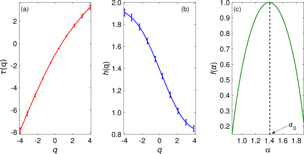
Supplementary Figure 8: Multifractal spectrum. Plots of (a) $\tau(q)$ versus $q$ and (b) $h(q)$ versus $q$ for a representative UCF. A few representative error bars shown in the plots represent the standard deviation in $\tau(q)$ and $h(q)$, respectively. (c) The singularity spectrum $f(\alpha)$ versus $\alpha$, obtained from the Legendre transform of $h(q)$ versus $q$, is shown. The black dashed vertical line marks the location of the maximum of $f(\alpha)$.

We now calculate the singularity spectrum as follows: We first calculate

$$\tau(q)=H(q)q-1.$$ (S10)

From this, we calculate the generalized Hurst exponent

$$h(q)=\frac{d\tau(q)}{dq}.$$ (S11)

In Supplementary Figure 8(a) we show plot of $\tau(q)$, for a representative UCF. By using this, and making use of the relation between $\tau(q)$ and $h(q)$ shown above, we obtain plots of $h(q)$ such as the one shown in Supplementary Figure 8(b).

$\alpha$ and $f(\alpha)$ follow from $\tau(q)$ and $h(q)$:

$$\alpha=\frac{d\tau(q)}{dq}=h(q);$$ (S12)

$$f(\alpha)=\alpha q-\tau(q).$$ (S13)

In Supplementary Figure 8(c) we show a plot of the multifractal singularity spectrum $f(\alpha)$, which shows a clear maximum at $f(\alpha_{0})=1$. It is important to keep in mind that the position of this maxima $\alpha_{0}\equiv h(0)$ depends on both the gate voltage $V_{\mathrm{G}}$ and the temperature $T$.

The error in $\tau(q)$ was estimated from the fitting error of the plot of $F_{q}(s)$ versus $s$ [Eqn. S9]. The error in $h(q)$ was obtained from error in $H(q)$ by using Eqn. S11. Absolute errors in $\tau(q)$ and $h(q)$ are represented using error-bars in Supplementary Figure 8(a) and (b), respectively. Finally, the error in the spectral width $\Delta\alpha$ is obtained by adding the error in $h(q)$, obtained at the two end values of q, i.e. $q=-4$ and $q=4$.

SUPPLEMENTARY NOTE 7 Multifractality of a randomly shuffled series

We generate a randomly shuffled sequence following the prescription mentioned below:

(i) We consider a data sequence $\{g(i)\}$, $i=1,2,...,N$.

(ii) We then generate a sequence $\{I(i)\}$ of length $N$, which is a random permutation of the positive integers from $1$ to $N$.

(iii) We then generate a new sequence $\{g_{\rm rs}(i)\}$, where $g_{\rm rs}(i)=g(I(i))$.

(iv) We repeat this shuffling for several times, to obtain the final randomly shuffled sequence.

Supplementary Figure 9 shows plots the generalized Hurst exponent $h(q)$ and the singularity spectrum $f(\alpha)$ of a UCF series (measured at $T$=20 mK and $\Delta V_{\mathrm{G}}=0.2~{}$V) and its randomly shuffled counterpart. The spectrum for the original data series is shown in blue continuous line, where as that for the randomly shuffled series is shown in red dashed line. For the original data series, $h(q)$ has a large range of values and the singularity spectrum $f(\alpha)$ is wide ($\Delta\alpha=1.05$ ) showing that the data series is multifractal. On the other hand, for the shuffled series, $h(q)$ is almost $q$-independent and $f(\alpha)$ is extremely narrow ($\Delta\alpha=0.05$), indicating a clear suppression of multifractality.

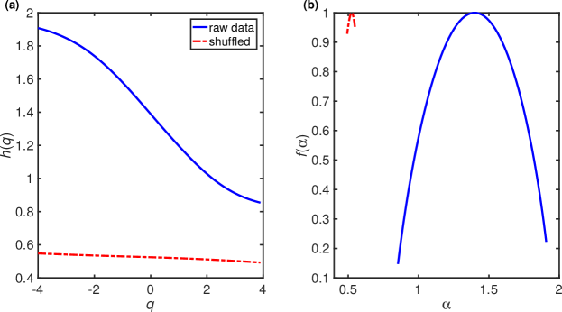
Supplementary Figure 9: Multifractality after shuffling. Plots of multifractality spectrum (a) $h(q)$ and (b) $f(\alpha)$ of an unshuffled UCF series (in blue continuous line) and a randomly shuffled series (in red, dashed line).

SUPPLEMENTARY NOTE 8 Monofractality versus Multifractality

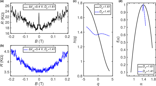
Supplementary Figure 10: (a) and (b) show plots of UCF measured on the single-layer graphene device G28M6 at two different values of $\Delta V_{\mathrm{G}}$, 0.4 V and 3.4 V respectively. The data were acquired at $T=20$ mK. (c) Plots of the order-$q$ scaling exponent $h(q)$ as a function of $q$; these exponents have been extracted from the plots (a) and (b). (d) Plots of the singularity spectrum $f(\alpha)$ versus $\alpha$, obtained from the Legendre transform of $h(q)$ versus $q$. Although the UCF measured at both these gate voltages are monofractal, it is multifractal only for the UCF measured very close to the Dirac point.

A näive characterization of the fractal property of a curve, say by the measurement of one fractal dimension, does not rule out multifractality of this curve, which requires the calculation of an infinite number of dimensions Grassberger and Procaccia (1983) (related to our $h(q)$). For monofractal scaling, a single dimension suffices (as, e.g., in the scaling of velocity structure functions in the inverse-cascade region of forced, two-dimensional fluid turbulence Kellay and Goldburg (2002); Boffetta and Ecke (2012)).

We note here, that for the single-layer graphene devices studied by us, even at the lowest temperature, we find $f(\alpha)$ depends on $\Delta V_{\mathrm{G}}$. All the UCFs measured by us are not multifractal; they are multifractal only in a narrow range of gate-voltages around the Dirac point. We show in Supplementary Figure 10 an example of a UCF, that is monofractal, but not multifractal. A UCF measured near the Dirac point ($\Delta V_{\mathrm{G}}=0.4$ V) [Supplementary Figure 10(a)] is multifractal, as seen in Supplementary Figure 10(c-d) (black solid lines). On the other hand, UCF measured away from the Dirac point ($\Delta V_{\mathrm{G}}=3.4$ V) [Supplementary Figure 10(b)], despite having a fractal dimension $D_{\mathrm{F}}=1.41$, is barely multifractal, as seen from the almost $q$ independent $h(q)$ and an extremely narrow singularity spectrum [Supplementary Figure 10(c-d) (blue dashed lines)].

References

References

- Evers and Mirlin (2008) F. Evers and A. D. Mirlin, Rev. Mod. Phys. 80, 1355 (2008).
- Ludwig et al. (1994) A. W. W. Ludwig, M. P. A. Fisher, R. Shankar, and G. Grinstein, Phys. Rev. B 50, 7526 (1994).
- Cheianov and Falko (2006) V. V. Cheianov and V. I. Falko, Phys. Rev. B 74, 041403 (2006).
- Aleiner and Efetov (2006) I. L. Aleiner and K. B. Efetov, Phys. Rev. Lett. 97, 236801 (2006).
- Katsnelson et al. (2006) M. I. Katsnelson, K. S. Novoselov, and A. K. Geim, Nat. Phys. 2, 620 (2006).
- Pereira et al. (2006) V. M. Pereira, F. Guinea, J. M. B. Lopes dos Santos, N. M. R. Peres, and A. H. Castro Neto, Phys. Rev. Lett. 96, 036801 (2006).
- Samaddar et al. (2016) S. Samaddar, I. Yudhistira, S. Adam, H. Courtois, and C. B. Winkelmann, Phys. Rev. Lett. 116, 126804 (2016).
- Bostwick et al. (2009) A. Bostwick, J. L. McChesney, K. V. Emtsev, T. Seyller, K. Horn, S. D. Kevan, and E. Rotenberg, Phys. Rev. Lett. 103, 056404 (2009).
- Jung et al. (2011) S. Jung, G. M. Rutter, N. N. Klimov, D. B. Newell, I. Calizo, A. R. Hight-Walker, N. B. Zhitenev, and J. A. Stroscio, Nat. Phys. 7, 245 (2011).
- Ponomarenko et al. (2011) L. A. Ponomarenko, A. K. Geim, A. A. Zhukov, R. Jalil, S. V. Morozov, K. S. Novoselov, I. V. Grigorieva, E. H. Hill, V. V. Cheianov, V. I. Fal/’ko, K. Watanabe, T. Taniguchi, and R. V. Gorbachev, Nat. Phys. 7, 958 (2011).
- Mandelbrot (1982) B. B. Mandelbrot, The Fractal Geometry of Nature (Freeman: San Francisco, 1982).
- Ivanov et al. (1999) P. C. Ivanov, L. A. N. Amaral, A. L. Goldberger, S. Havlin, M. G. Rosenblum, Z. R. Struzik, and H. E. Stanley, Nature 399, 461 (1999).
- Lawrence et al. (1993) J. Lawrence, A. Ruzmaikin, and A. Cadavid, The Astrophysical Journal 417, 805 (1993).
- Oudjemia et al. (2013) S. Oudjemia, J. M. Girault, N. e. Derguini, and S. Haddab, in 8th International Workshop on Systems, Signal Processing and their Applications (2013) pp. 244–249.
- Frisch (1995) U. Frisch, Turbulence: the legacy of AN Kolmogorov (Cambridge university press, 1995).
- Benzi et al. (1984) R. Benzi, G. Paladin, G. Parisi, and A. Vulpiani, J. Phys. A: Math. Gen. 17, 3521 (1984).
- Castellani and Peliti (1986) C. Castellani and L. Peliti, J. Phys. A: Math. Gen. 19, L429 (1986).
- Janssen (1998) M. Janssen, Phys. Rep. 295, 1 (1998).
- Mirlin (2000) A. D. Mirlin, Phys. Rep. 326, 259 (2000).
- Grussbach and Schreiber (1995) H. Grussbach and M. Schreiber, Phys. Rev. B 51, 663 (1995).
- Burmistrov et al. (2015) I. S. Burmistrov, I. V. Gornyi, and A. D. Mirlin, Phys. Rev. B 91, 085427 (2015).
- Burmistrov et al. (2013) I. S. Burmistrov, I. V. Gornyi, and A. D. Mirlin, Phys. Rev. Lett. 111, 066601 (2013).
- Gruzberg et al. (2013) I. A. Gruzberg, A. D. Mirlin, and M. R. Zirnbauer, Phys. Rev. B 87, 125144 (2013).
- Barrios-Vargas and Naumis (2014) J. E. Barrios-Vargas and G. G. Naumis, 2D Mater. 1, 011009 (2014).
- Facchini et al. (2007) A. Facchini, S. Wimberger, and A. Tomadin, Physica A 376, 266 (2007).
- Monthus and Garel (2009) C. Monthus and T. Garel, Phys. Rev. B 79, 205120 (2009).
- Rammal et al. (1985) R. Rammal, C. Tannous, P. Breton, and A. M. S. Tremblay, Phys. Rev. Lett. 54, 1718 (1985).
- Roux et al. (1991) S. Roux, A. Hansen, and E. L. Hinrichsen, Phys. Rev. B 43, 3601 (1991).
- Brandes et al. (1994) T. Brandes, L. Schweitzer, and B. Kramer, Phys. Rev. Lett. 72, 3582 (1994).
- Polyakov (1998) D. G. Polyakov, Phys. Rev. Lett. 81, 4696 (1998).
- Hegger et al. (1996) H. Hegger, B. Huckestein, K. Hecker, M. Janssen, A. Freimuth, G. Reckziegel, and R. Tuzinski, Phys. Rev. Lett. 77, 3885 (1996).
- Micolich et al. (2001) A. P. Micolich, R. P. Taylor, A. G. Davies, J. P. Bird, R. Newbury, T. M. Fromhold, A. Ehlert, H. Linke, L. D. Macks, W. R. Tribe, E. H. Linfield, D. A. Ritchie, J. Cooper, Y. Aoyagi, and P. B. Wilkinson, Phys. Rev. Lett. 87, 036802 (2001).
- Sachrajda et al. (1998) A. S. Sachrajda, R. Ketzmerick, C. Gould, Y. Feng, P. J. Kelly, A. Delage, and Z. Wasilewski, Phys. Rev. Lett. 80, 1948 (1998).
- Ketzmerick (1996) R. Ketzmerick, Phys. Rev. B 54, 10841 (1996).
- Ujiie et al. (2008) Y. Ujiie, N. Yumoto, T. Morimoto, N. Aoki, and Y. Ochiai, J. Phys. Conf. Ser. 109, 012035 (2008).
- Meiss and Ott (1986) J. D. Meiss and E. Ott, Physica D 20, 387 (1986).
- Geisel et al. (1987) T. Geisel, A. Zacherl, and G. Radons, Phys. Rev. Lett. 59, 2503 (1987).
- Novoselov et al. (2005) K. Novoselov, A. K. Geim, S. Morozov, D. Jiang, M. Katsnelson, I. Grigorieva, S. Dubonos, and A. Firsov, Nature 438, 197 (2005).
- Chen et al. (2010) Y.-F. Chen, M.-H. Bae, C. Chialvo, T. Dirks, A. Bezryadin, and N. Mason, Journal of Physics: Condensed Matter 22, 205301 (2010).
- Berger et al. (2006) C. Berger, Z. Song, X. Li, X. Wu, N. Brown, C. Naud, D. Mayou, T. Li, J. Hass, A. N. Marchenkov, E. H. Conrad, P. N. First, and W. A. de Heer, Science 312, 1191 (2006), http://science.sciencemag.org/content/312/5777/1191.full.pdf .
- Bohra et al. (2012) G. Bohra, R. Somphonsane, D. K. Ferry, and J. P. Bird, Applied Physics Letters 101, 093110 (2012), http://dx.doi.org/10.1063/1.4748167 .
- Tikhonenko et al. (2008) F. V. Tikhonenko, D. W. Horsell, R. V. Gorbachev, and A. K. Savchenko, Phys. Rev. Lett. 100, 056802 (2008).
- Horsell et al. (2009) D. Horsell, A. Savchenko, F. Tikhonenko, K. Kechedzhi, I. Lerner, and V. Fal ko, Solid State Communications 149, 1041 (2009), recent Progress in Graphene Studies.
- Gorbachev et al. (2007) R. V. Gorbachev, F. V. Tikhonenko, A. S. Mayorov, D. W. Horsell, and A. K. Savchenko, Phys. Rev. Lett. 98, 176805 (2007).
- Mohanty and Webb (2003) P. Mohanty and R. A. Webb, Phys. Rev. Lett. 91, 066604 (2003).
- Mohanty and Webb (1997) P. Mohanty and R. A. Webb, Phys. Rev. B 55, R13452 (1997).
- Pierre et al. (2003) F. Pierre, A. B. Gougam, A. Anthore, H. Pothier, D. Esteve, and N. O. Birge, Phys. Rev. B 68, 085413 (2003).
- Liu et al. (2016) B. Liu, R. Akis, D. K. Ferry, G. Bohra, R. Somphonsane, H. Ramamoorthy, and J. P. Bird, Journal of Physics: Condensed Matter 28, 135302 (2016).
- Gu and Zhou (2010) G.-F. Gu and W.-X. Zhou, Phys. Rev. E 82, 011136 (2010).
- Zhou (2009) W.-X. Zhou, EPL (Europhysics Letters) 88, 28004 (2009).
- Grassberger and Procaccia (1983) P. Grassberger and I. Procaccia, Phys. Rev. Lett. 50, 346 (1983).
- Kellay and Goldburg (2002) H. Kellay and W. I. Goldburg, Reports on Progress in Physics 65, 845 (2002).
- Boffetta and Ecke (2012) G. Boffetta and R. E. Ecke, Annual Review of Fluid Mechanics 44, 427 (2012), https://doi.org/10.1146/annurev-fluid-120710-101240 .
- Heller (1984) E. J. Heller, Phys. Rev. Lett. 53, 1515 (1984).
- Harper (1955) P. G. Harper, Proc. Phys. Soc. London, Sect. A 68, 879 (1955).
- Hofstadter (1976) D. R. Hofstadter, Phys. Rev. B 14, 2239 (1976).
- Ostlund et al. (1983) S. Ostlund, R. Pandit, D. Rand, H. J. Schellnhuber, and E. D. Siggia, Phys. Rev. Lett. 50, 1873 (1983).
- Sena et al. (2010) S. H. R. Sena, J. M. P. Jr, G. A. Farias, M. S. Vasconcelos, and E. L. Albuquerque, J. Phys.: Condens. Matter 22, 465305 (2010).
- Zurek (1981) W. H. Zurek, Phys. Rev. D 24, 1516 (1981).
- Huang et al. (2009) L. Huang, Y.-C. Lai, D. K. Ferry, S. M. Goodnick, and R. Akis, Phys. Rev. Lett. 103, 054101 (2009).
- Ostlund and Pandit (1984) S. Ostlund and R. Pandit, Phys. Rev. B 29, 1394 (1984).
- Brandes et al. (1996) T. Brandes, B. Huckestein, and L. Schweitzer, Ann. Phys. 508, 633 (1996).
- Harris and Aharony (1987) A. B. Harris and A. Aharony, Europhys. Lett. 4, 1355 (1987).
- Benenti et al. (2001) G. Benenti, G. Casati, I. Guarneri, and M. Terraneo, Phys. Rev. Lett. 87, 014101 (2001).
- Ugeda et al. (2010) M. M. Ugeda, I. Brihuega, F. Guinea, and J. M. Gómez-Rodríguez, Phys. Rev. Lett. 104, 096804 (2010).
- Shytov et al. (2007) A. V. Shytov, M. I. Katsnelson, and L. S. Levitov, Phys. Rev. Lett. 99, 236801 (2007).
- Das Sarma et al. (2011) S. Das Sarma, S. Adam, E. H. Hwang, and E. Rossi, Rev. Mod. Phys. 83, 407 (2011).
- Casati et al. (2000) G. Casati, I. Guarneri, and G. Maspero, Phys. Rev. Lett. 84, 63 (2000).
- Lai et al. (1992) Y.-C. Lai, R. Blümel, E. Ott, and C. Grebogi, Phys. Rev. Lett. 68, 3491 (1992).
- Nakayama and Yakubo (2013) T. Nakayama and K. Yakubo, Fractal Concepts in Condensed Matter Physics, Springer Series in Solid-State Sciences (Springer Berlin Heidelberg, 2013).

References

- Beenakker and van Houten (1991) C. Beenakker and H. van Houten, in Semiconductor Heterostructures and Nanostructures, Solid State Physics, Vol. 44, edited by H. Ehrenreich and D. Turnbull (Academic Press, 1991) pp. 1 – 228.
- Tikhonenko et al. (2008) F. V. Tikhonenko, D. W. Horsell, R. V. Gorbachev, and A. K. Savchenko, Phys. Rev. Lett. 100, 056802 (2008).
- Horsell et al. (2009) D. Horsell, A. Savchenko, F. Tikhonenko, K. Kechedzhi, I. Lerner, and V. Fal ko, Solid State Communications 149, 1041 (2009), recent Progress in Graphene Studies.
- Chen et al. (2010) Y.-F. Chen, M.-H. Bae, C. Chialvo, T. Dirks, A. Bezryadin, and N. Mason, Journal of Physics: Condensed Matter 22, 205301 (2010).
- Berger et al. (2006) C. Berger, Z. Song, X. Li, X. Wu, N. Brown, C. Naud, D. Mayou, T. Li, J. Hass, A. N. Marchenkov, E. H. Conrad, P. N. First, and W. A. de Heer, Science 312, 1191 (2006), http://science.sciencemag.org/content/312/5777/1191.full.pdf .
- Bohra et al. (2012) G. Bohra, R. Somphonsane, D. K. Ferry, and J. P. Bird, Applied Physics Letters 101, 093110 (2012), http://dx.doi.org/10.1063/1.4748167 .
- Gorbachev et al. (2007) R. V. Gorbachev, F. V. Tikhonenko, A. S. Mayorov, D. W. Horsell, and A. K. Savchenko, Phys. Rev. Lett. 98, 176805 (2007).
- Mohanty and Webb (2003) P. Mohanty and R. A. Webb, Phys. Rev. Lett. 91, 066604 (2003).
- Mohanty and Webb (1997) P. Mohanty and R. A. Webb, Phys. Rev. B 55, R13452 (1997).
- Pierre et al. (2003) F. Pierre, A. B. Gougam, A. Anthore, H. Pothier, D. Esteve, and N. O. Birge, Phys. Rev. B 68, 085413 (2003).
- Liu et al. (2016) B. Liu, R. Akis, D. K. Ferry, G. Bohra, R. Somphonsane, H. Ramamoorthy, and J. P. Bird, Journal of Physics: Condensed Matter 28, 135302 (2016).
- Ketzmerick (1996) R. Ketzmerick, Phys. Rev. B 54, 10841 (1996).
- Kantelhardt (2012) J. W. Kantelhardt, in Mathematics of complexity and dynamical systems (Springer, 2012) pp. 463–487.
- Grassberger and Procaccia (1983) P. Grassberger and I. Procaccia, Phys. Rev. Lett. 50, 346 (1983).
- Kellay and Goldburg (2002) H. Kellay and W. I. Goldburg, Reports on Progress in Physics 65, 845 (2002).
- Boffetta and Ecke (2012) G. Boffetta and R. E. Ecke, Annual Review of Fluid Mechanics 44, 427 (2012), https://doi.org/10.1146/annurev-fluid-120710-101240 .