Regularized Greedy Column Subset Selection

Abstract

The Column Subset Selection Problem provides a natural framework for unsupervised feature selection. Despite being a hard combinatorial optimization problem, there exist efficient algorithms that provide good approximations. The drawback of the problem formulation is that it incorporates no form of regularization, and is therefore very sensitive to noise when presented with scarce data. In this paper we propose a regularized formulation of this problem, and derive a correct greedy algorithm that is similar in efficiency to existing greedy methods for the unregularized problem. We study its adequacy for feature selection and propose suitable formulations. Additionally, we derive a lower bound for the error of the proposed problems. Through various numerical experiments on real and synthetic data, we demonstrate the significantly increased robustness and stability of our method, as well as the improved conditioning of its output, all while remaining efficient for practical use.

Ordozgoiti et al.

1 Introduction

Among dimensionality reduction methods, those that select features instead of transforming them are convenient when preserving the semantic meaning of the variables is necessary. This, together with the abundance of large, unlabelled data sets, motivates the study of efficient unsupervised feature selection algorithms. Column Subset Selection is a combinatorial optimization problem that translates naturally to this purpose. It can be formulated as follows.

Problem 1.

Column Subset Selection Problem (CSSP). Given a matrix $A\in\mathbb{R}^{m\times n}$ and a positive integer $k$ smaller than the rank of $A$, let $\mathcal{A}_{k}$ denote the set of $m\times k$ matrices comprised of $k$ columns of $A$. Find

$$\underset{C\in\mathcal{A}_{k}}{\operatorname*{\arg\!\min}}\|A-CC^{+}A\|_{F}$$ (1)

where $C^{+}$ is the Moore-Penrose pseudoinverse of $C$.

This objective is akin to the singular value decomposition, but we constrain the basis vectors to be a selection of the columns originally present in our data matrix. It attains its minimum at the matrix $C$, composed by a subset of $k$ columns of $A$, with which we can best approximate the rest of the columns of $A$.

Problem 1 is a hard combinatorial problem, known to be UG-hard [1]. Only very recently did a claimed proof of NP-completeness of the decision version appear [2]. Therefore, for practical applications it is interesting to find efficient approximation algorithms. One example is a greedy algorithm, which in addition to having approximation guarantees [3], works very well in practice and can be implemented very efficiently [4].

An important drawback of problem 1 is that the approximation $CC^{+}A$ is unregularized, and therefore the coefficient matrix $C^{+}A$ can grow unbounded without incurring any penalty. This means that if the matrix $A$ contains contingent quirks (e.g. noisy measurements), any algorithm might yield spuriously expressive column subsets, which might later perform badly on new data.

Our purpose in this paper is to endow the CSSP with a regularization penalty so that column subsets leading to parsimonious approximations are favored. In addition, we want to derive an algorithm that is comparably efficient to the existing greedy method for the CSSP, and correctly optimizes each subproblem corresponding to the greedy approximation.

The main contributions of this paper can be summarized as follows:

• We propose a regularized formulation of the column subset selection problem.

• We show that assuming certain conditions are met, there exists an algorithm that solves the greedy optimization objective at iteration $t$ in $O(\min\{np,n^{2}\})$ time complexity, where $p=\max\{m,t\}$. In addition, we show that a procedure can be developed to ensure that said conditions are met as we build the set $S$ incrementally, thus allowing us to derive an efficient, correct greedy algorithm for problem.

• We discuss how this approach, if adopted in a naive fashion, can be inadequate for feature selection and propose an alternative objective, as well as an algorithm, to overcome this drawback.

• We offer a lower bound for the error of the proposed problems, which can serve to inform a stopping criterion.

2 Related work

Many works have explored the problem of unsupervised feature selection in the past decades, some focusing on the column subset selection problem and others following different approaches. Here we offer a brief overview.

2.1 Locality and cluster structure preservation

Many proposals try to find algorithms that preserve the manifold structure of the data, choosing features that preserve local affinity between data instances. A seminal work in this field proposes to build a k-nearest neighbor matrix [5]. Then, features preserving the structure of said matrix are kept. The feature scores can be computed as a function of the Laplacian of the graph encoded by the nearest neighbor matrix. In [6] this approach is generalized in a framework that applies to both supervised and unsupervised feature selection. In the supervised case, the similarity between instances belonging to the same class is represented with a per-class constant value. Furthermore, the features can be ranked based on their similarity to the eigenvectors of the normalized Laplacian of the similarity graph. The notion of choosing features by examining their ability to preserve the local connectivity or manifold structure of the data is explored further in various works, considering a penalty term to exploit unlabelled data in an SVM [7], performing sparse regression on the spectral embedding of the data [8], [9] or optimizing a discriminator matrix with an $\ell{2,1}$-norm penalty [10] [11]. Many of these approaches were shown to be realizations of a general framework, as well as ineffective to detect redundancies, by Zhao et al. [12].

The use of the $\ell{2,1}$-norm penalty on a coefficient matrix is convenient for feature selection, as it promotes row sparsity, and can be found in several other works [13], [14], [15], [16], [17], [18]. Some recent works propose the use of a regularized coefficient matrix to choose features that can reconstruct the entire data set well in a manner that is similar to the problem we tackle in this paper [18], [19].

2.2 Column subset selection

The column subset selection problem (CSSP) has also received significant attention over the last few years. Its origins can be traced back to factorizations with column pivoting to isolate well-conditioned column subsets [20]. More recently, several methods have been proposed to approximate a matrix based on a subset of its entries, generally building upon the ideas introduced in the seminal work of Frieze and Vempala [21]. One such method is the CUR matrix decomposition [22]. Other methods that explicitly target the CSSP with approximation guarantees have been proposed [23] [24]. An adequate alternative for practical applications is the greedy algorithm, which generally provides good subset choices and can be implemented very efficiently [4]. It has been shown that this algorithm also enjoys approximation guarantees [25] [3]. Recently, an efficient local-search method was shown empirically to outperform other existing approaches in terms of the objective function [26]. A lower bound for the recovered matrix norm was proved in subsequent work [27].

Most existing proposals for the CSSP attempt to solve the optimization problem directly. The inconvenient of this approach is that the resulting approximation model is unregularized, and is therefore sensitive to irrelevant idiosyncrasies of the input data, like outliers and noise, especially when data are scarce. In this paper we propose the addition of a regularization term to the problem formulation, making the solutions less sensitive to undesirable peculiarities of the available data. In addition, we show that the new problem can still be approximately optimized very efficiently in a greedy fashion, which makes our method well-suited for practical use.

3 Greedy column subset selection

Notation

• $A_{i:}$ is the $i$-th row and $A_{:i}$ the $i$-th column of $A$.

• $A_{ij}$ is the entry in the $i$-th row and $j$-th column of matrix $A$.

• $\mathcal{P}(S)$: the power set of set $S$

• $|S|$ is the cardinality of set $S$

• Given a matrix $A\in\mathbb{R}^{m\times n}$ and a set $S\subset\{1,\dots,n\}$, $A_{S}$ is the $m\times k$ matrix comprised of the columns of $A$ whose indices are in the set $S$.

• If $x_{i}$ is a vector, then $x_{ii}$ is its $i$-th element.

• $[n]$ denotes the subset of $\mathbb{N}$ defined as $\mathbb{N}\cap[1,n]$,

• Given vectors $x,y$ of the same dimension, $x\circ y$ denotes the element-wise product of $x$ and $y$.

• Given two matrices $A$ and $B$, $(A~{}B)$ is the matrix resulting from appending the columns of $B$ to $A$. E.g., if $A\in\mathbb{R}^{m\times n},B\in\mathbb{R}^{m\times k}$, then $(A~{}B)\in\mathbb{R}^{m\times n+k}$ and consists of the columns of both matrices. The notation $\left(\begin{array}[]{c}A\\ B\end{array}\right)$, is analogous, but denotes row-wise, instead of column-wise, concatenation.

The greedy maximization of the CSSP objective is based on the following observation. Let $A\in\mathbb{R}^{m\times n}$ and let $C$ be a matrix composed by a proper subset of the columns of $A$. Let $\tilde{C}$ denote the matrix that results from adding an additional column of $A$ to $C$, that is $\tilde{C}=(C~{}A_{:w})$ for some column index $w$. Then

$$A-\tilde{C}\tilde{C}^{+}A=A-CC^{+}A-E_{:w}E_{:w}^{+}E$$ (2)

where $E=A-CC^{+}A$. This is easily seen considering that $CC^{+}$ is a projection onto the space spanned by the columns of $C$, and therefore all the columns of $E$ are orthogonal to those of $CC^{+}A$.

Equation 2 implies that we can easily perform a greedy selection of columns, by updating $A$ at each step to obtain the corresponding residual $E$ and choosing a column $w$ of $E$ to minimize $\|E-E_{:w}E_{:w}^{+}E\|_{F}^{2}$. Furthermore, the minimizing column can be found efficiently. In [4] it is shown that

$$\operatorname*{\arg\!\min}_{i}\|E-E_{:w}E_{:w}^{+}E\|_{F}^{2}=\operatorname*{\arg\!\max}_{i}\frac{\|G_{:i}\|_{2}^{2}}{G_{ii}}$$ (3)

where $G=E^{T}E$. In addition, the values of $\|G_{:i}\|_{2}^{2}$ and $G_{ii}$ for all $i$ can be updated efficiently every time we incorporate a new column to our subset.

3.1 Regularized greedy column subset selection

In this section we propose a modification of the CSSP objective to enable regularization. The approach is as follows. If we observe that $CC^{+}A=C(C^{T}C)^{-1}C^{T}A$ (whenever the inverse exists), we can consider Tikhonov regularization for linear regression (ridge regression) and reformulate the CSSP as follows:

Problem 2.

Given a matrix $A\in\mathbb{R}^{m\times n}$ and a positive integer $k\leq n$ and $\lambda\in\mathbb{R}$, let $\mathcal{A}_{k}$ denote the set of $m\times k$ matrices comprised of $k$ columns of $A$. Find

$$\underset{C\in\mathcal{A}_{k}}{\operatorname*{\arg\!\min}}\|A-C(C^{T}C+\lambda I)^{-1}C^{T}A\|_{F}$$ (4)

This problem is equivalent to the CSSP, but using a regularized approximation of the target matrix. By introducing the term $\lambda$, we penalize subsets that would require very large coefficient matrices. We can therefore tune its value to trade off between goodness of fit and model complexity.

The problem of this approach is that the greedy algorithm described in section 3 is no longer applicable. The reason is that this greedy method, as described by Farahat et al. [4], relies heavily on the fact that $CC^{+}$ is a projection. The corresponding term of the regularized formulation, $(C^{T}C+\lambda I)^{-1}C^{T}$, ceases to be a projection whenever $\lambda>0$. Therefore, equations 2 and 3 no longer hold.

Before we proceed, we will define the following function in order to simplify our notation. For a matrix $A\in\mathbb{R}^{m\times n}$,

$$f_{A}:\mathcal{P}([n])\times\mathbb{R} \rightarrow\mathbb{R}^{m\times n}$$

$$S,\lambda \mapsto f_{A}(S,\lambda)=A_{S}(A_{S}^{T}A_{S}+\lambda I)^{-1}A_{S}^{T}A$$

where $\mathcal{P}([n])$ is the power set of $[n]$. That is, given a set $S$ and a regularizing term $\lambda$, $f_{A}(S,\lambda)$ denotes the approximation of $A$ obtained using the columns indexed by $S$, regularized using $\lambda$.

Our goal in this paper is to derive an efficient greedy algorithm for problem 2. In essence, we need an algorithm that solves the following sub-problem:

Problem 3.

Given a matrix $A\in\mathbb{R}^{m\times n}$ and a set $S\subset[n]$, find

$$\operatorname*{\arg\!\min}_{i}\|A-f_{A}(S\cup\{i\},\lambda)\|_{F}^{2}$$ (5)

Given a column subset $S$, this problem is solved by finding the best addition to said subset. Therefore, a correct greedy algorithm should solve this problem at each iteration. Obviously, we can solve problem 3 simply by inspecting the value of the objective function for all possible choices of $i$. This method, however, involves considerable computations, as each candidate requires (for $|S|=t$) matrix products of complexity $O(mnt)$ and $O(nt^{2})$ and a matrix inversion of complexity $O(t^{3})$, in addition to the matrix subtraction and the computation of the norm. In sum, each iteration of the resulting algorithm would take $O(\max\{mn^{2}t,n^{2}t^{2}\})$ operations. The algorithm we propose here solves problem 3 in $O(\min\{np,n^{2}\})$ time, where $p=\max\{m,t\}$.

4 Algorithms for regularized greedy column subset selection

Let us assume we are running a greedy algorithm that has so far completed $t$ iterations, i.e., we have a set $S$ of $t$ elements. We want to solve problem 3, that is,

$$\operatorname*{\arg\!\min}_{i}\|A-f_{A}(S\cup\{i\},\lambda)\|_{F}^{2}$$

As said before, we can of course do this by inspecting the value of this objective for all possible choices. However, this would be computationally costly. If we define $C_{i}=A_{S\cup\{i\}}$, in order to do this we would need to compute the inverse of $C_{i}^{T}C_{i}+\lambda I$ for all choices of $i$. We can start our derivation by attempting to circumvent these matrix inversions, which we can accomplish as follows. We define

$$\hat{A}=\left(\begin{array}[]{c}A\\ \sqrt{\lambda}I\end{array}\right)$$

and $\hat{C}_{i}=\hat{A}_{S\cup\{i\}}$.

If we observe that

$$C_{i}^{T}C_{i}+\lambda I=\hat{C}_{i}^{T}\hat{C}_{i}$$

then we can take advantage of the following fact. Let us denote $w=A_{:w},\hat{w}=\hat{A}_{:w}$ (here we use column indices and the corresponding vectors interchangeably). Since $\hat{C}_{w}=\hat{A}_{S\cup\{w\}}=(\tilde{C}\mbox{ }\tilde{w})$, then it is well known [28] that

$$(C_{w}^{T}C_{w}+\lambda I)^{-1}=(\hat{C}_{w}^{T}\hat{C}_{w})^{-1}=\left(\begin{array}[]{cc}(C^{T}C+\lambda I)^{-1}+\frac{vv^{T}}{\alpha_{w}}&\hskip 10.00002pt-\frac{v}{\alpha_{w}}\\ -\frac{v^{T}}{\alpha_{w}}&\hskip 18.00005pt\frac{1}{\alpha_{w}}\end{array}\right)$$

where $\alpha_{w}=\hat{w}^{T}\hat{w}-\hat{w}^{T}\hat{C}(C^{T}C+\lambda I)^{-1}\hat{C}^{T}\hat{w}$ and $v=(C^{T}C+\lambda I)^{-1}C^{T}w$. (Note that $C^{T}w=\hat{C}^{T}\hat{w}$ because the extension of $w$ is multiplied by zero).

Relying on this expression for the inverse of $C_{w}^{T}C_{w}+\lambda I$, we can look for a solution to problem 3 that does not need to explicitly compute the value of the objective for all choices of $i$. For brevity, let us define $A^{(t)}=f_{A}(S,\lambda)$ and $A^{(t+1)}=f_{A}(S\cup\{w\},\lambda)$. First, observe that (for a detailed derivation, refer to the appendix)

$$A^{(t+1)}=C_{w}(C_{w}^{T}C_{w}+\lambda I)^{-1}C_{w}^{T}A$$

$$=~{} A^{(t)}+\frac{1}{\alpha_{w}}(A^{(t)}_{:w}-w)(A^{(t)}_{:w}-w)^{T}A$$ (6)

Let $d_{i}=(A^{(t)}_{:i}-A_{:i})\in\mathbb{R}^{m}$. Then the next column choice is yielded by

$$\operatorname*{\arg\!\min}\|A-A^{(t+1)}\|_{F}^{2}$$

$$= \operatorname*{\arg\!\min}_{i}tr(A^{T}A)-tr(A^{T}A^{(t)})-tr(\frac{1}{\alpha_{i}}A^{T}d_{i}d_{i}^{T}A)$$

$$-tr((A^{T})^{(t)}A)-tr(\frac{1}{\alpha_{i}}A^{T}d_{i}d_{i}^{T}A)$$

$$+tr((A^{T})^{(t)}A^{(t)})+tr(\frac{1}{\alpha_{i}}(A^{T})^{(t)}d_{i}d_{i}^{T}A)+tr(\frac{1}{\alpha_{i}}A^{T}d_{i}d_{i}^{T}A^{(t)})$$

$$+tr(\frac{1}{\alpha_{i}^{2}}A^{T}d_{i}d_{i}^{T}d_{i}d_{i}^{T}A)$$ (7)

We define $x_{i}=A^{T}d_{i}\in\mathbb{R}^{n}$, $\tilde{x}_{i}=(A^{(t)})^{T}d_{i}\in\mathbb{R}^{n}$. Dropping irrelevant constants from the previous equality,

$$\operatorname*{\arg\!\min}\|A-A^{(t+1)}\|_{F}^{2}$$

$$= -2tr(\frac{1}{\alpha_{i}}A^{T}d_{i}d_{i}^{T}A)+2tr(\frac{1}{\alpha_{i}}(A^{T})^{(t)}d_{i}d_{i}^{T}A)+tr(\frac{1}{\alpha_{i}^{2}}A^{T}d_{i}d_{i}^{T}d_{i}d_{i}^{T}A)$$

$$= \operatorname*{\arg\!\min}_{i}\frac{2}{\alpha_{i}}\tilde{x}_{i}^{T}x_{i}-\frac{2}{\alpha_{i}}\|x_{i}\|_{2}^{2}+\frac{1}{\alpha_{i}^{2}}\|d_{i}\|_{2}^{2}\|x_{i}\|_{2}^{2}$$

$$= \operatorname*{\arg\!\min}_{i}\frac{2}{\alpha_{i}}\tilde{x}_{i}^{T}x_{i}+(\frac{-2}{\alpha_{i}}+\frac{1}{\alpha_{i}^{2}}(\tilde{x}_{ii}-x_{ii}))x_{i}^{T}x_{i}+\lambda$$ (8)

Equality 8 provides a surrogate of problem 3, i.e., the problem we need to solve at each iteration in order to implement a correct greedy algorithm for problem 2. In particular, equality 8 shows that the solution to the problem 3 can be found as a function of $x_{i},\tilde{x}_{i}$ and $\alpha_{i}$ for $i=1,\dots,n$. Our concern now is to develop a procedure to find the value of these variables at each iteration without incurring too much computational cost.

We have

$$\tilde{x}_{i}^{T}x_{i} =d_{i}^{T}A^{(t)}A^{T}d_{i}$$

$$x_{i}^{T}x_{i} =d_{i}^{T}AA^{T}d_{i}$$

For notational convenience, we define the matrices $X,\tilde{X}$ and $D$, whose columns are the vectors $x_{i},\tilde{x}_{i}$ and $d_{i}$, $i=1,\dots,n$ respectively. First, observe from equality 6 that

$$A^{(t+1)}=A^{(t)}+\frac{1}{\alpha_{w}}d_{w}d_{w}^{T}A$$

Hence,

$$A^{T}A^{(t+1)}=A^{T}A^{(t)}+\frac{1}{\alpha_{w}}x_{w}x_{w}^{T}$$ (9)

And

$$(A^{T}A)^{(t+1)}=(A^{T}A)^{(t)}+\frac{1}{\alpha_{w}}\tilde{x}_{w}x_{w}^{T}+\frac{1}{\alpha_{w}}x_{w}\tilde{x}_{w}^{T}+\frac{1}{\alpha_{w}^{2}}x_{w}d_{w}^{T}d_{w}x_{w}^{T}$$ (10)

So finally,

$$X^{(t+1)} =A^{T}D^{(t+1)}$$

$$=A^{T}D^{(t)}+A^{T}A+\frac{1}{\alpha_{w}}x_{w}x_{w}^{T}-A^{T}A$$

$$=X^{(t)}+\frac{1}{\alpha_{w}}x_{w}x_{w}^{T}=X^{(0)}+\sum_{i=0}^{t}\left(\frac{1}{a_{w}}x_{w}x_{w}^{T}\right)^{(i)}$$ (11)

And

$$\tilde{X}^{(t+1)} =(A^{T}D)^{(t+1)}$$

$$=(A^{T}D)^{(t)}+\frac{1}{\alpha_{w}}\tilde{x}_{w}x_{w}^{T}+\frac{1}{\alpha_{w}}x_{w}\tilde{x}_{w}^{T}+\frac{1}{\alpha_{w}^{2}}x_{w}d_{w}^{T}d_{w}x_{w}^{T}-\frac{1}{\alpha_{w}}x_{w}x_{w}^{T}$$

$$=\sum_{i=0}^{t}\left(\frac{1}{\alpha_{w}}\tilde{x}_{w}x_{w}^{T}+\frac{1}{\alpha_{w}}x_{w}\tilde{x}_{w}^{T}+\frac{1}{\alpha_{w}^{2}}x_{w}d_{w}^{T}d_{w}x_{w}^{T}-\frac{1}{\alpha_{w}}x_{w}x_{w}^{T}\right)^{(i)}$$ (12)

Expressions 11 and 12 allow us to compute the variables involved in problem 8 efficiently as more columns are greedily added to the final set. Specifically, it is easy to see that

$$(x_{i}^{T}\tilde{x}_{i})^{(t+1)}=x_{i}^{T}\tilde{x}_{i}$$

$$+\left(x_{i}+\frac{1}{\alpha_{w}}x_{w}x_{wi}\right)^{T}\left(\tilde{x}_{i}+\frac{1}{\alpha_{w}}\tilde{x}_{w}x_{w}^{T}+\frac{1}{\alpha_{w}}x_{w}\tilde{x}_{w}^{T}+\frac{1}{\alpha_{w}^{2}}x_{w}x_{w}^{T}(\tilde{x}_{ww}-x_{ww})-\frac{1}{\alpha_{w}}x_{w}x_{w}^{T}\right)$$

$$=x_{i}^{T}\tilde{x}_{i}+\frac{1}{\alpha_{w}}(x_{i}^{T}\tilde{x}_{w}x_{wi}+x_{i}^{T}x_{w}(\tilde{x}_{wi}-x_{wi})+\tilde{x}_{i}^{T}x_{w}x_{wi})$$

$$+\frac{1}{\alpha_{w}^{2}}(x_{i}^{T}x_{w}x_{wi}(\tilde{x}_{ww}-x_{ww})+x_{w}^{T}x_{w}x_{wi}\tilde{x}_{wi}+x_{w}^{T}\tilde{x}_{w}(x_{wi})^{2}-x_{w}^{T}x_{w}(x_{wi})^{2})$$

$$+\frac{1}{\alpha_{w}^{3}}x_{w}^{T}x_{w}(x_{wi})^{2}(\tilde{x}_{ww}-x_{ww})$$ (13)

$$(x_{i}^{T}x_{i})^{(t+1)} =x_{i}^{T}x_{i}+\frac{2x_{wi}}{\alpha_{w}}x_{i}^{T}x_{w}+\left(\frac{x_{wi}}{\alpha_{w}}\right)^{2}x_{w}^{T}x_{w}$$ (14)

All elements on the r.h.s. of equalities 14 and 13 correspond to iteration $t$. The superindex has been omitted for clarity. Furthermore, in equation 14 we consider the values for the already chosen indices to be irrelevant in order to simplify the expression.

The inner products involved in these updates can also be computed efficiently by making use of equalities (11) and (12) as follows:

$$x_{i}^{T}x_{w}:=\left(x_{i}^{(0)}\right)^{T}(x_{w})^{(t)}+\left(\sum_{j=0}^{t}\left(\frac{1}{a_{w}}x_{w}x_{wi}\right)^{(j)}\right)^{T}(x_{w})^{(t)}$$

$$x_{i}^{T}\tilde{x}_{w}:=\left(x_{i}^{(0)}\right)^{T}(\tilde{x}_{w})^{(t)}+\left(\sum_{j=0}^{t}\left(\frac{1}{a_{w}}x_{w}x_{wi}\right)^{(j)}\right)^{T}(\tilde{x}_{w})^{(t)}$$

$$\tilde{x}_{i}^{T}x_{w}:=\sum_{j=0}^{t}\left(\frac{1}{\alpha_{w}}\tilde{x}_{w}x_{wi}+\frac{1}{\alpha_{w}}x_{w}\tilde{x}_{wi}+\frac{\tilde{x}_{ww}-x_{ww}}{\alpha_{w}^{2}}x_{w}x_{wi}-\frac{1}{\alpha_{w}}x_{w}x_{wi}\right)^{(j)}(x_{w})^{(t)}$$

Based on the equalities presented above, we can state and prove our main result regarding the existence of an efficient algorithm for problem 3. The proof is constructive and provides the necessary equalities for implementing the algorithm.

Theorem 1.

Given a matrix $A\in\mathbb{R}^{m\times n}$, $\lambda\in\mathbb{R}$ and a set $S$ of cardinality $t\leq n$, let us assume the following values, as defined above, are known:

1. $X^{(0)}=-A^{T}A$

2. $x_{w(i)}^{(i)},\tilde{x}_{w(i)}^{(i)},\alpha_{w(i)}^{(i)},i=0,\dots,t-1$

where $w(i)$ is the index of the $(i+1)$-th column added to the set $S$. Then there exists an algorithm that solves problem 3 in $O(\min\{np,n^{2}\})$ time, where $p=\max\{m,t\}$.

Proof.

In order to relieve the notation, we employ $x_{w}^{(i)}$ to denote $x_{w(i)}^{(i)}$.

Equality 8 gives an expression that reveals the optimum of the objective function of problem 3. We now show that this expression can be computed in $O(\min\{np,n^{2}\}))$ time.

First, observe from equalities 11 and 12 that the values of $x_{w}$ and $\tilde{x}_{w}$ for this iteration can be computed in $O(nt)$ time complexity as follows:

$$x_{w}^{(t)}:=X^{(0)}_{:w}+\sum_{j=0}^{t-1}\left(\frac{1}{a_{w}}x_{w}x_{ww}^{T}\right)^{(j)}$$

$$\tilde{x}_{w}^{(t)}:=\sum_{j=0}^{t-1}\left(\frac{x_{ww}}{\alpha_{w}}\tilde{x}_{w}+\frac{\tilde{x}_{ww}}{\alpha_{w}}x_{w}+\frac{\tilde{x}_{ww}-x_{ww}}{\alpha_{w}^{2}}x_{w}x_{ww}-\frac{x_{ww}}{\alpha_{w}}x_{w}\right)^{(j)}$$

We now define the matrices $W,\tilde{W}$ whose columns are respectively $x_{w}^{(0)},\dots,x_{w}^{(t-1)}$ and $\tilde{x}_{w}^{(0)},\dots,\tilde{x}_{w}^{(t-1)}$. We also define the diagonal matrix

$$B=\left(\begin{array}[]{ccc}\frac{1}{\alpha_{w}^{(0)}}&&\\ &\ddots&\\ &&\frac{1}{\alpha_{w}^{(t-1)}}\end{array}\right)$$

and the column-scaled matrices $W_{\alpha}=WB$, $\tilde{W}_{\alpha}=\tilde{W}B$.

The following equalities can be easily verified (from here on, we use $x_{w},\tilde{x}_{w}$ to denote $x_{w}^{(t)},\tilde{x}_{w}^{(t)}$).

$$\left(\sum_{j=0}^{t-1}\left(\frac{1}{a_{w}}x_{w}x_{wi}\right)^{(j)}\right)^{T}x_{w}^{(t)}=W_{i:}W_{\alpha}^{T}x_{w}^{(t)}$$

$$\left(\sum_{j=0}^{t-1}\left(\frac{1}{a_{w}}x_{w}x_{wi}\right)^{(j)}\right)^{T}\tilde{x}_{w}^{(t)}=W_{i:}W_{\alpha}^{T}\tilde{x}_{w}^{(t)}$$

Combined with equalities 11 and 12, this implies the following:

$$(x^{T}_{1}x_{w}^{(t)},\dots,x^{T}_{n}x_{w}^{(t)})^{T}=X^{(0)}x_{w}^{(t)}+WW_{\alpha}^{T}x_{w}^{(t)}$$

$$(x^{T}_{1}\tilde{x}_{w}^{(t)},\dots,x^{T}_{n}\tilde{x}_{w}^{(t)})^{T}=X^{(0)}\tilde{x}_{w}^{(t)}+WW_{\alpha}^{T}\tilde{x}_{w}^{(t)}$$

And similarly,

$$(\tilde{x}^{T}_{1}x_{w}^{(t)},\dots,\tilde{x}^{T}_{n}x_{w}^{(t)})^{T}=\tilde{X}^{T}x_{w}^{(t)}$$

$$=W\tilde{W}_{\alpha}^{T}x_{w}^{(t)}+\tilde{W}W_{\alpha}^{T}x_{w}^{(t)}+\alpha^{-1}(\tilde{x}_{w}^{(t)}-x_{w}^{(t)})WW_{\alpha}^{T}x_{w}^{(t)}+WW_{\alpha}^{T}x_{w}^{(t)}$$

Since $X^{(0)}\in\mathbb{R}^{n\times n}$, $W,\tilde{W}\in\mathbb{R}^{n\times t}$ and $x_{w}^{(t)},\tilde{x}_{w}^{(t)}\in\mathbb{R}^{n\times 1}$, these equalities can be computed in $O(2n^{2}+8nt)=O(n^{2})$. If $n>m$, instead of storing $X^{(0)}$ we can explicitly compute $-A^{T}Ax_{w}^{(t)}$ and $-A^{T}A\tilde{x}_{w}^{(t)}$, resulting in $O(\max\{mn,nt\})$ time complexity for the greedy step.

Using the variables $x^{T}_{i}x_{w}^{(t)}$, $x^{T}_{i}\tilde{x}_{w}^{(t)}$ and $\tilde{x}^{T}_{i}x_{w}^{(t)}$, which we have computed for $i=1,\dots,n$, we can now compute $\tilde{x}_{i}^{T}x_{i}$ and $x_{i}^{T}x_{i}$ as shown in equalities 13 and 14. Finally, from equalities 11 and 12 and the definition of $\alpha_{i}$, it is easily verified that

$$x_{ii}^{(t)}=\left(x_{ii}+\frac{1}{(\alpha_{w})}x_{wi}^{2}\right)^{(t-1)}$$

$$\tilde{x}_{ii}^{(t)}=\left(\tilde{x}_{ii}+\frac{2\tilde{x}_{wi}x_{wi}-x_{wi}^{2}}{(\alpha_{w})}+x_{wi}^{2}\frac{(\tilde{x}_{ii}-x_{ii})}{\alpha_{w}^{2}}\right)^{(t-1)}$$

$$\alpha_{i}=\lambda-x_{ii}$$

These operations are easily seen to require $O(n)$ time complexity if computed for all $i$.

Having computed all these variables, we can now compute the value of expression 8 for all $i$ in a straightforward manner, thus completing the proof.

∎

By theorem 1, if we store the value of $x_{w},\tilde{x}_{w}$ and $\alpha_{w}$ at each iteration, we can efficiently find the best column addition for the regularized column subset selection formulation. This allows us to derive a greedy algorithm for problem 2.

4.1 Algorithm

Input: $A\in\mathbb{R}^{m\times n},k\in\mathbb{N},k\leq n$

1. $X\leftarrow-A^{T}A$; $\alpha\leftarrow\lambda-diag(X)$; $x_{w}^{(0)}\leftarrow X_{:w}$; $\tilde{x}_{w}^{(0)}\leftarrow 0$

2. Compute $x_{i}^{T}x_{i},i=1,\dots,n$

3. Choose the first column, $w\leftarrow\operatorname*{\arg\!\min}_{i}\frac{-2}{\alpha_{i}}-\frac{x_{ii}}{\alpha_{i}^{2}}x_{i}^{T}x_{i}+\lambda$

4. $S\leftarrow\{w\};\omega\leftarrow{\bf 0}\in\mathbb{R}^{n}$

5. for $t=1,\dots,k-1$

6. $x_{w}\leftarrow x_{w}^{(t-1)}$

7. $\tilde{x}_{w}\leftarrow\tilde{x}_{w}^{(t-1)}$

8. $\beta\leftarrow Xx_{w}+WW_{\alpha}^{T}x_{w}$

9. $\gamma\leftarrow X\tilde{x}_{w}+WW_{\alpha}^{T}\tilde{x}_{w}$

10. $\delta\leftarrow W\tilde{W}_{\alpha}^{T}x_{w}+\tilde{W}W_{\alpha}^{T}x_{w}+\alpha^{-1}(\tilde{x}_{w}-x_{w})WW_{\alpha}^{T}x_{w}+WW_{\alpha}^{T}x_{w}$

11. $\begin{aligned} \omega\leftarrow\omega&+\alpha_{w}^{-1}(\gamma\circ x_{w}+\beta\circ(\tilde{x}_{w}-x_{w})+\delta\circ x_{w})\\ &+\alpha_{w}^{-2}(\beta\circ x_{w}(\tilde{x}_{ww}-x_{ww})+\beta_{w}x_{w}\circ\tilde{x}_{w}+(\gamma_{w}-\beta_{w})x_{w}^{2})\\ &+\alpha_{w}^{-3}\beta_{w}x_{w}\circ x_{w}(\tilde{x}_{ww}-x_{ww})\end{aligned}$

12. $\psi\leftarrow\psi+\frac{2}{\alpha_{w}}x_{w}\circ\beta+\frac{\beta_{w}}{\alpha_{w}^{2}}x_{w}\circ x_{w}$

13. for $i=1,\dots,n$

14. $x_{ii}\leftarrow x_{ii}+\frac{1}{\alpha_{w}}x_{wi}^{2}$

15. $\tilde{x}_{ii}\leftarrow\tilde{x}_{ii}+\frac{2}{\alpha_{w}}\tilde{x}_{wi}x_{wi}+\frac{\tilde{x}_{ii}-x_{ii}}{\alpha_{w}^{2}}x_{wi}^{2}-\frac{1}{\alpha_{w}}x_{wi}$

16. $\alpha_{i}\leftarrow\lambda-x_{ii}$

17. $w\leftarrow\operatorname*{\arg\!\min}_{i}\frac{2}{\alpha_{i}}\omega_{i}+(\frac{-2}{\alpha_{i}}+\frac{1}{\alpha_{i}^{2}}(\tilde{x}_{ii}-x_{ii}))\psi_{i}+\lambda$

18. $S\leftarrow S\cup\{w\}$

19. $x_{w}^{(t)}\leftarrow X_{:w}+\sum_{j=0}^{t-1}\left(\frac{1}{a_{w}}x_{w}x_{ww}^{T}\right)^{(j)}$

20. $\tilde{x}_{w}^{(t)}\leftarrow\sum_{j=0}^{t-1}\left(\frac{x_{ww}}{\alpha_{w}}\tilde{x}_{w}+\frac{\tilde{x}_{ww}}{\alpha_{w}}x_{w}+\frac{\tilde{x}_{ww}-x_{ww}}{\alpha_{w}^{2}}x_{w}x_{ww}-\frac{x_{ww}}{\alpha_{w}}x_{w}\right)^{(j)}$

4.2 An appropriate formulation for feature selection

The purpose of this algorithm is that of selecting a few variables and approximating the rest. In the context of practical applications of feature selection, we can consider that the chosen variables become available and do not need to be approximated. However, the penalty of the regularized formulation causes the chosen variables to be imperfectly estimated. This means that in optimizing the objective in problem 3, we are taking into account an error that should not be made in reality, thus providing a potentially mistaken choice.

This can be illustrated with an example. Consider the following matrix.

$$\left(\begin{array}[]{c c c c}1&0&0&1\\ 0&1&0&0\\ 1&0&1&1\\ 1&1&0&0\end{array}\right)$$

and the set $S=\{1,2\}$. The solution to problem 3 is given by adding column 4 to $S$. However, if we don’t consider the error made in the approximation of the chosen columns, the best choice is column 3. As stated above, in a feature selection setting we would not want to consider the approximation error of the chosen columns, as we can assume the corresponding variables to be available.

For this reason, we propose the following alternative problem formulation.

Problem 4.

Given a matrix $A\in\mathbb{R}^{m\times n}$ and a positive integer $k$ smaller than the rank of $A$, and defining $\bar{S}=[n]\backslash S$, find

$$\underset{S,|S|=k}{\operatorname*{\arg\!\min}}\|A_{\bar{S}}-A_{S}(A_{S}^{T}A_{S}+\lambda I)^{-1}A_{S}^{T}A_{\bar{S}})\|_{F}^{2}$$ (15)

This is equivalent to problem 2, but it discards the error made in approximating the chosen variables. Fortunately, the algorithm proposed in section 4 can be easily modified to greedily optimize this objective. We show how by induction on $t$.

At iteration $t$, consider equation 6.

$$A^{(t+1)}=A^{(t)}+\frac{1}{\alpha_{w}}d_{w}x^{T}$$

If we assume that the chosen columns (those in $S$) are approximated exactly in $A^{(t)}$, i.e. $A_{S}=A^{(t)}_{S}$, these need not be modified. Therefore, we can simply set the corresponding positions of $x$ to zero, and these columns will not be altered. For the next iteration, however, we are adding a new column to $S$, which we can denote $w$. Thus, we need that $A_{S\cup\{w\}}=A^{(t+1)}_{S\cup\{w\}}$.

We have $d_{w}=A^{(t)}_{:w}-w$. Therefore, if $x_{ww}=-\alpha_{w}$,

$$A^{(t)}_{:w}+\frac{1}{\alpha_{w}}d_{w}x_{ww}=A^{(t)}_{:w}-d_{w}=w$$

That is, by setting $x_{S}=0$ and $x_{ww}=-\alpha_{w}$ we ensure that the chosen columns are considered to be perfectly approximated. If we set $x_{ww}^{(0)}=-\alpha_{w}^{(0)}$, then we ensure that the first chosen column is approximated with no error, providing the basis for our inductive argument.

By defining $(x^{*})^{(t)}$ to be equal to $x^{(t)}$ but with the previously described replacements, we can easily modify our algorithm to ensure that the column chosen at each iteration is the one that greedily optimizes problem 4. We now detail the necessary modifications:

1. $x_{i}^{T}x_{w}^{*}:=\left(x_{i}^{(0)}\right)^{T}(\tilde{x}_{w}^{*})^{(t)}+\left(\sum_{i=0}^{t-1}\left(\frac{1}{a_{w}}x_{w}x_{w}^{T}\right)^{(i)}\right)^{T}(\tilde{x}_{w}^{*})^{(t)}$

2. $\tilde{x}_{i}^{T}x_{w}:=\sum_{i=0}^{t-1}\left(\frac{1}{\alpha_{w}}\tilde{x}_{w}x_{w}^{T}+\frac{1}{\alpha_{w}}x_{w}\tilde{x}_{w}^{T}+\frac{1}{\alpha_{w}^{2}}x_{w}d_{w}^{T}d_{w}x_{w}^{T}-\frac{1}{\alpha_{w}}x_{w}x_{w}^{T}\right)^{(i)}(x_{w}^{*})^{(t)}$

3. $x_{w}^{*}:=x_{w}$; $x_{wi}^{*}=0,i\in S$; $x_{ww}^{*}=-\alpha_{w}$

4. $\tilde{x}_{w}:=\sum_{i=0}^{t}\left(\frac{1}{\alpha_{w}}\tilde{x}_{w}x_{w}^{T}+\frac{1}{\alpha_{w}}x_{w}^{*}\tilde{x}_{w}^{T}+\frac{1}{\alpha_{w}^{2}}x_{w}^{*}d_{w}^{T}d_{w}x_{w}^{T}-\frac{1}{\alpha_{w}}x_{w}^{*}x_{w}^{T}\right)^{(i)}$

Equality 13:

$$(x_{i}^{T}\tilde{x}_{i})^{(t+1)}=x_{i}^{T}\tilde{x}_{i}$$

$$+\left(x_{i}+\frac{1}{\alpha_{w}}x_{w}x_{wi}\right)^{T}\left(\tilde{x}_{i}+\frac{1}{\alpha_{w}}\tilde{x}_{w}x_{w}^{T}+\frac{1}{\alpha_{w}}x_{w}\tilde{x}_{w}^{T}+\frac{1}{\alpha_{w}^{2}}x_{w}x_{w}^{T}(\tilde{x}_{ww}-x_{ww})-\frac{1}{\alpha_{w}}x_{w}x_{w}^{T}\right)$$

$$=x_{i}^{T}\tilde{x}_{i}+\frac{1}{\alpha_{w}}(x_{i}^{T}\tilde{x}_{w}x_{wi}+x_{i}^{T}x_{w}^{*}(\tilde{x}_{wi}-x_{wi})+\tilde{x}_{i}^{T}x_{w}x_{wi})$$

$$+\frac{1}{\alpha_{w}^{2}}(x_{i}^{T}x_{w}^{*}x_{wi}(\tilde{x}_{ww}-x_{ww})+x_{w}^{T}x_{w}^{*}x_{wi}\tilde{x}_{wi}+x_{w}^{T}\tilde{x}_{w}(x_{wi})^{2}-x_{w}^{T}x_{w}^{*}(x_{wi})^{2})$$

$$+\frac{1}{\alpha_{w}^{3}}x_{w}^{T}x_{w}^{*}(x_{wi})^{2}(\tilde{x}_{ww}-x_{ww})$$

Equality 14:

$$(x_{i}^{T}x_{i}^{*})^{(t+1)}$$ (16)

$$=x_{i}^{T}x_{i}^{*}+\frac{2x_{wi}^{*}}{\alpha_{w}}x_{i}^{T}\tilde{x}_{w}+\left(\frac{x_{wi}^{*}}{\alpha_{w}}\right)^{2}x_{w}^{T}x_{w}-\left(\frac{x_{wi}}{\alpha_{w}}x_{wS}^{T}x_{wS}\right)^{2}-(x_{wi}+x_{wi}\frac{x_{ww}}{\alpha_{w}})^{2}$$

4.3 Choosing the value of $k$

In order to decide when to stop the algorithm, we can monitor the loss of the approximation at each iteration, i.e. $\|A-A^{(t)}\|_{F}^{2}$. Computing this quantity at each iteration, however, can be costly. Fortunately, we can take advantage of the variables involved in the proposed algorithm to efficiently track the exact value of the loss.

By equation (6) we can easily see that

$$\|A-A^{(t)}\|_{F}^{2} =\|A-A^{(t-1)}-\frac{1}{\alpha_{w}}d_{w}x_{w}^{T}\|_{F}^{2}$$

$$=\left(A-A^{(t-1)}-\frac{1}{\alpha_{w}}d_{w}x_{w}^{T}\right)^{T}\left(A-A^{(t-1)}-\frac{1}{\alpha_{w}}d_{w}x_{w}^{T}\right)$$

$$=\|A-A^{(t-1)}\|_{F}^{2}-\frac{2}{\alpha_{w}}x_{w}^{T}x_{w}+\frac{2}{\alpha_{w}}\tilde{x}_{w}^{T}x_{w}+\frac{\tilde{x}_{ww}-x_{ww}}{\alpha_{w}}x_{w}^{T}x_{w}$$

For problem 4, this equality becomes

$$\|A-A^{(t)}\|_{F}^{2}=\|A-A^{(t-1)}\|_{F}^{2}-\frac{2}{\alpha_{w}}x_{w}^{T}x_{w}^{*}+\frac{2}{\alpha_{w}}\tilde{x}_{w}^{T}x_{w}^{*}+\frac{\tilde{x}_{ww}-x_{ww}}{\alpha_{w}}\left(x_{w}^{*}\right)^{T}x_{w}^{*}$$

where $x^{*}$ is defined as in section 4.2.

This means that we can compute the loss at each iteration as a function of its previous value and some readily available variables. The loss before the first iteration is simply the squared norm of the data matrix, which can be computed as $trA^{T}A=-trX$.

In section 4.4 we discuss how this quantity can be used to determine when to stop iterating.

4.4 Lower bound for the error

In the conventional formulation of the CSSP, the approximation error eventually reaches zero as we add columns to the basis subset. However, the introduction of the regularizing term bars the approximation from being perfect. For this reason, even if we can track the loss as detailed in section 4.3, it can be difficult to determine how much of an improvement can still be made. In other words, in problem 1 we can evaluate the expressive power of our column subset by checking how far the error is from zero. On the contrary, in the case of problem 2 we do not know what this ideal lower bound is.

In the case of problem 4, the loss can of course reach zero, but rather artificially (when $k=n$, we simply evaluate the error over zero columns of the matrix). Here we propose a lower bound for the objective function of problem 4 at each iteration, providing insight on the manner in which $\lambda$ interacts with the approximation error. This bound can be easily extended to problem 2.

Lemma 1.

Given a matrix $A\in\mathbb{R}^{m\times n}$, a regularization term $\lambda\in\mathbb{R}$ and a set $S$ such that $|S|=k\leq n$. let $\sigma_{i}$ denote the $i$-th largest singular value of $A$. Then

$$\|A_{\bar{S}}-A_{S}(A_{S}^{T}A_{S}+\lambda I)^{-1}A_{S}^{T}A_{\bar{S}})\|_{F}^{2}\geq\lambda^{2}\sum_{i=k+1}^{n}\left(\frac{\sigma_{i}}{\sigma_{i}^{2}+\lambda}\right)^{2}$$ (17)

Proof.

Let us assume $A=A_{S}$, which corresponds to the best possible approximation we can obtain of the columns of $A$ using a subset of its columns as a basis. If $A=U\Sigma V^{T}$ is the singular value decomposition of $A$,

$$A-A(A^{T}A+\lambda I)^{-1}A^{T}A=U\Sigma V^{T}-U\Sigma(\Sigma^{2}+\lambda I)^{-1}\Sigma^{2}V^{T}$$

$$=U\Sigma V^{T}-U\left(\begin{array}[]{ccc}\frac{\sigma_{1}^{3}}{\sigma_{1}^{2}+\lambda}&&\\ &\ddots&\\ &&\frac{\sigma_{n}^{3}}{\sigma_{n}^{2}+\lambda}\end{array}\right)V^{T}$$

$$=U\left(\begin{array}[]{ccc}\frac{\sigma_{1}\lambda}{\sigma_{1}^{2}+\lambda}&&\\ &\ddots&\\ &&\frac{\sigma_{n}\lambda}{\sigma_{n}^{2}+\lambda}\end{array}\right)V^{T}$$

The error incurred by approximating $A$ by itself using the regularized formulation is therefore exactly

$$\|A-f_{A}([n],\lambda)\|_{F}^{2}=\lambda^{2}\sum_{i=1}^{n}\left(\frac{\sigma_{i}}{\sigma_{i}^{2}+\lambda}\right)^{2}$$

Now consider that

$$\|A_{\bar{S}}-A_{S}(A_{S}^{T}A_{S}+\lambda I)^{-1}A_{S}^{T}A_{\bar{S}}\|_{F}^{2} \geq\|A_{\bar{S}}-A(A^{T}A+\lambda I)^{-1}A^{T}A_{\bar{S}}\|_{F}^{2}$$

$$\geq\lambda^{2}\sum_{i=k+1}^{n}\left(\frac{\sigma_{i}}{\sigma_{i}^{2}+\lambda}\right)^{2}$$

The second inequality holds because of the interlacing inequalities of the singular values [29], and because $A_{\bar{S}}-A(A^{T}A+\lambda I)^{-1}A^{T}A_{\bar{S}}$ is an $m\times(n-k)$ submatrix of $A-f_{A}([n],\lambda)$. ∎

To adapt this bound to problem 2, we simply need to extend the summation of the last inequality over all singular values. The resulting expression for the error bound vanishes when $\lambda=0$ and approaches $\sum_{i}\sigma^{2}$ as $\lambda\rightarrow\infty$. This is of course consistent with the problem formulation. Observe that in the first case, we are measuring the error incurred by approximating $A_{S}$ using its full span. In the second case, we approximate $A$ with a vanishing matrix, thus making the error equal to $\|A\|_{F}^{2}=\sum_{i}\sigma_{i}^{2}$.

This bound can be used to choose the value of $k$ if the input data set is suitable. If at some point the algorithm attains a value of the objective in problem 4 that is close to this bound, then the present matrix has almost as much representative power as the full column set, thus making the addition of more columns innecessary.

5 Numerical experiments

In order to validate our claims, we perform a series of numerical experiments. Specifically, we aim to assess the following aspects:

• Generalization ability. We test the ability of the proposed algorithm to choose variables that can approximate well not only the input data (training data) but also future observations (test data).

• Stability. We test how robust our algorithm is to noisy variations in the data.

• Conditioning. We measure the conditioning of the selected submatrix, defined as the ratio between the largest and the smallest singular values.

• Running time. We evaluate the running time of our algorithm with respect to different input parameters.

• Applications. We evaluate the effectiveness of our algorithm as a preprocessing step for clustering and its ability to reconstruct partially observed images.

To this end, we employed a variety of well-known data sets. We now briefly describe them, and indicate the preprocessing operations and the training/test splits for each of them.

• Isolet [30]. This data set consists of a collection of spoken letter recordings by various individuals, each represented by a set of features. The data were used as distributed. The variables are real-valued between -1 and 1. For the test set, we respected the split proposed by the authors.

• MNIST [31]. Images of handwritten digits. The data were divided by 255 to ensure that all values be between 0 and 1. The training/test split provided by the authors was respected.

• Yale Face Extended [32]. Images of faces. The data were divided by 255 to ensure that all values be between 0 and 1. The first 1200 instances were used for training. The rest for testing.

• ORL [33]. Ten different images of each of 40 distinct subjects. The data were divided by 255 to ensure that all values be between 0 and 1. The first 300 instances were used for training. The rest for testing.

• COIL-20 [34]. Images of objects of different categories. The data were divided by 255 to ensure that all values be between 0 and 1. The data were split into two halves for training and testing, ensuring class balance between both sets. We reduce the size of the images to 64$\times$64.

• Online News Popularity [35]. Statistics associated to news articles. All variables were standardized to zero mean and unit variance. The first 30,000 instances were used for training. The rest for testing.

Table 1 summarizes the employed data sets.

Table 1: Employed datasets.

Dataset	Variables	Train	Test
ORL	1024	300	100
MNIST	784	60,000	10,000
YaleB	1024	1200	1214
OnlineNews	58	30,000	30,000
IsoLet	617	5200	1559
COIL-20	4096	300	100

We consider two algorithms:

• GCSS: The unregularized greedy algorithm for problem 1. We use a Python implementation of the algorithm described by Farahat et al. [4].

• RGCSS: The algorithm proposed in this paper to solve problem 4 (iterating until the desired number of columns is chosen). We use a Python implementation. In all experiments we use the algorithm adapted to optimize problem 4.

5.1 Generalization ability

In our first set of experiments, we evaluate whether the regularized formulation and the corresponding algorithm select columns that produce models with better generalization ability. To this end, we run the algorithms, both GCSS and RGCSS, on small samples of the training splits of the data sets, and then measure the ability of the resulting models to approximate the rest of the features of the test split.

Given an input matrix $A$, a test matrix $B$, a number $k\in\mathbb{N}$ and a value of $\lambda\in\mathbb{R}$, assume the algorithm being run outputs the set $S$. Then we measure the loss as

$$L(S)=\|B-B_{S}(A_{S}^{T}A_{S}+\lambda I)^{-1}A_{S}^{T}A\|_{F}^{2}$$

Notice that for both the unregularized and the regularized algorithms, we measure the loss using a regularized approximation. This is because even though the unregularized version does not attempt to optimize this objective, the approximation on the test split will generally be much better if we introduce the regularization term $\lambda$, thus providing a fairer comparison. In doing so, we set the bar higher for our algorithm.

For all data sets, we run the algorithms on $2^{i}\%,i=0,\dots,4$ of the training data, for $k=2^{i},i=4,\dots,9$, and then measure the loss on the test split. It should be noted that we simply set $\lambda=1$ for all cases. However, better results might be obtained by fine-tuning this parameter. In order to assess the improvement brought by the regularized variant, we measure the relative improvement as follows. Let $S_{N}$ be the set output by the GCSS, and $S_{R}$ the set output by RGCSS. Then the relative improvement is defined as

$$100\times\frac{L(S_{N})-L(S_{R})}{L(S_{N})}$$

In order to provide a better estimate of this value, we run the algorithms 50 times on different random samples of the training set and replace $L(S_{N})$ and $L(S_{R})$ with their averages.

Figure 1 illustrate the results. For each data set, we show the relative improvement for the different fractions of the training set. It can be seen that the regularizing penalty yields significant improvements, especially when training data are scarce and $k$ is large. Notice the different scale on the plots corresponding to OnlineNews and MNIST, where the improvement was more moderate.

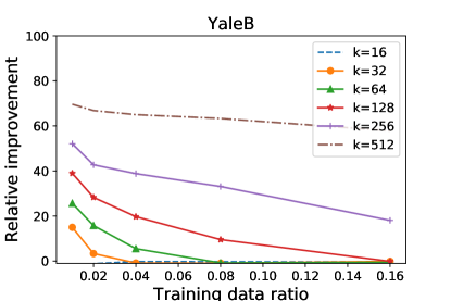
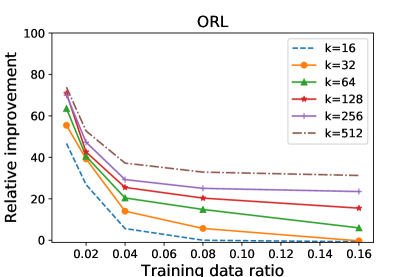
(a)

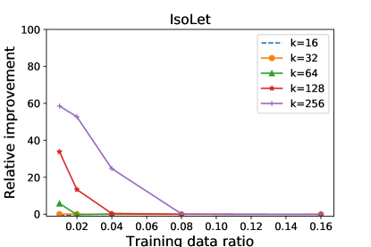
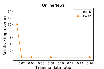
(b)

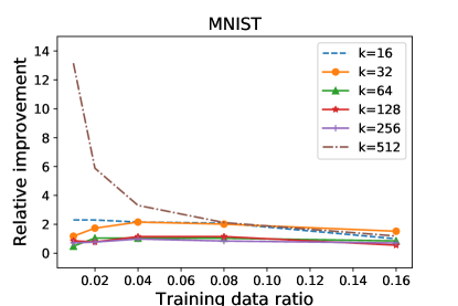
(c)

Figure 1: Relative improvement of the regularized variant

5.2 Stability

As discussed above, instances of the unregularized formulation of the column subset selection problem (problem 1) where $n\gg m$ are inconvenient. In this set of experiments, we aim to verify whether the regularized formulation and the corresponding algorithm improves the stability of the results. In order to tests this, we perturb the input data to see how the algorithms behave in the face of noise.

To measure the stability of each of the algorithms, we run them on $s$ different instances of the perturbed matrix and measure the average pairwise Jaccard index, which we define below. Given two sets $S_{1},S_{2}$, the Jaccard index is measured as

$$J(S_{1},S_{2})=\frac{|S_{1}\cap S_{2}|}{|S_{1}\cup S_{2}|}$$

Given a collection of sets $S_{1},\dots,S_{s}$, we define the average pairwise Jaccard index as

$$\bar{J}(S_{1},\dots,S_{s})=\frac{1}{s(s-1)}\sum_{i}^{s}\sum_{j}^{s}J(S_{i},S_{j})\mathbb{I}\{i\neq j\}$$

where $I\{i\neq j\}$ is 1 if $i\neq j$, 0 otherwise. To make this index more meaningful, we calculate its expected value assuming the column subsets are chosen uniformly at random. Given a matrix of $n$ columns, assume we want to select a subset of size $k$. If we pick two subsets of $[n]$ at random, $S_{1}$ and $S_{2}$, there are ${n\choose k}^{2}$ possible outcomes. Out of these, the number of pairs that have $k-p$ elements in common is

$${n\choose k}{k\choose p}{{n-k}\choose p}$$

To see this, observe that for each of the ${n\choose k}$ possible values of $S_{1}$, $S_{2}$ must have $p$ out of $k$ elements that are not in $S_{1}$, and those can be any of the remaining $n-k$ ones. Therefore, the expected value of the size of the intersection between two subsets drawn uniformly at random is

$$\mathbb{E}[S_{1}\cap S_{2}]=\sum_{p=0}^{k}\frac{(k-p){k\choose p}{{n-k}\choose p}}{{n\choose k}}$$

Now, the Jaccard index of each of those pairs is the size of the intersection divided by the size of the union. Hence, given $n$ and $k$,

$$\mathbb{E}[J]=\sum_{p=0}^{k}\frac{(k-p){k\choose p}{{n-k}\choose p}}{{n\choose k}(k+p)}$$

We can now measure the stability of the algorithms by running them on different perturbations of the input matrix, and then comparing the average pairwise Jaccard index of the resulting subsets with the expected value of the Jaccard index. We consider the case where $n>m$, that is, the input matrix has more columns than rows. To this end, we take random samples of 100 rows of each training data set and set $k=m$. In the case of OnlineNews, since $n<100$, we take $k=m=n/2$. Note that the case $k>m$ becomes pathological in the unregularized formulation, since any column choice once the span of the data has been covered is equally inocuous. Therefore, as $k$ grows beyond the value of $m$, the Jaccard index for the unregularized formulation will approach $\mathbb{E}[J]$ if ties are broken arbitrarily.

We take the input data set and perturb it with a matrix whose entries are independently sampled from a Gaussian distribution with zero mean and a standard deviation of $10^{-3}$. As explained above, we apply $s$ different perturbations to the input data and run the algorithms on each of them, thus obtaining $s$ different subsets for each algorithm. We set $s=100$ and measure the average pairwise Jaccard index. Table 5 shows the results. We also show the expected value of the Jaccard index to know how close to a random choice each algorithm is. We run this experiment for $\lambda=0$ (i.e. the unregularized algorithm by Farahat et al. [4]), $\lambda=1$ and $\lambda=10$. It can be seen that the regularized formulation significantly improves the stability of the results.

5.3 Conditioning

The conditioning of a matrix can be loosely understood as a measure of numerical rank defficiency. Formally, given a matrix $C$ of rank $k$, we define its conditioning, or its condition number, as $\kappa(C)=\frac{\sigma_{1}(C)}{\sigma_{k}(C)}$. Ill-conditioned matrices, that is, with a large condition number, are prone to significant numerical errors when involved in the solution of linear systems.

We compute the condition number of the submatrices of the training set selected by both algorithms, regularized and unregularized. We run the algorithm 50 times on different random samplings of the training set and report the minimum, average and maximum across all runs in table 2. The results clearly reveal that the regularization term encourages the selection of significantly better-conditioned column subsets.

In order to avoid overcrowding the table we only report the results for $k=16,32$, as they are illustrative of the general behaviour of the algorithms in this regard.

An interesting fact revealed by our experiments is the following: in cases where $k>m$, the unregularized formulation of the problem is ill-posed. In terms of the objective function, once the $m$-dimensional subspace spanned by the matrix has been covered, any subsequent column choice is equally good. The unregularized algorithm therefore yields particularly poorly conditioned subsets (see e.g. YaleB, $0.01*m$, $k=16$, $\lambda=0$ in table 2. What is surprising is that in these situations, the regularized variant produces column subsets that lead to well-conditioned matrices even in the test set. An example of the obtained condition numbers on submatrices of the test set is shown in table 3.

Table 2: Condition number of the matrices output by the unregularized and the regularized algorithms. For each experiment we report the minimum, average and maximum (min / avg / max) of 50 runs on different random samplings.

		$k=16$		$k=32$
Sample size	Dataset	$GCSS$	$RGCSS$	$GCSS$	$RGCSS$
0.01*m	ORL	13.07 / 338.94 / 3127.57	4.45 / 6.28 / 10.71	33.92 / 116.77 / 240.82	3.90 / 5.10 / 7.68
	MNIST	130.88 / 142.34 / 153.50	5.74 / 6.13 / 6.56	10.22 / 146.46 / 241.65	10.22 / 10.90 / 11.80
	YaleB	243.81 / 12186.18 / 48241.03	31.97 / 183.84 / 1019.68	214.28 / 1218.04 / 2575.45	10.10 / 63.30 / 272.59
	OnlineNews	2.37 / 3.63 / 5.33	2.37 / 3.39 / 4.59	4.67 / 5.86 / 7.43	4.58 / 5.71 / 7.32
	Isolet	12.66 / 19.91 / 29.78	11.58 / 14.75 / 17.96	43.04 / 77.20 / 133.39	31.35 / 39.31 / 58.30
0.04*m	ORL	119.35 / 2331.63 / 20602.93	55.78 / 90.22 / 187.40	183.43 / 985.98 / 4140.42	20.59 / 27.88 / 42.15
	MNIST	136.33 / 147.26 / 161.20	5.61 / 5.90 / 6.27	227.12 / 235.81 / 247.82	9.36 / 10.03 / 10.40
	YaleB	29.62 / 35.36 / 46.36	24.32 / 32.24 / 41.23	99.93 / 134.32 / 185.35	76.28 / 103.24 / 139.18
	OnlineNews	2.46 / 3.17 / 4.07	2.46 / 3.01 / 3.91	3.99 / 4.82 / 5.86	3.98 / 4.72 / 5.51
	Isolet	10.82 / 13.24 / 16.66	10.42 / 12.52 / 16.53	20.40 / 24.28 / 28.62	20.38 / 23.58 / 27.96
0.16*m	ORL	61.95 / 74.08 / 90.82	41.89 / 60.14 / 86.10	178.82 / 233.01 / 304.82	131.69 / 175.00 / 210.30
	MNIST	130.80 / 146.03 / 151.36	5.55 / 18.69 / 134.06	225.88 / 235.61 / 244.84	9.95 / 55.10 / 241.62
	YaleB	22.11 / 24.50 / 28.54	20.93 / 24.29 / 28.38	40.26 / 43.60 / 51.41	38.01 / 41.91 / 48.99
	OnlineNews	2.45 / 2.80 / 3.34	2.45 / 2.80 / 3.34	3.78 / 4.38 / 5.12	3.77 / 4.24 / 5.12
	Isolet	9.58 / 10.74 / 11.93	9.58 / 10.74 / 11.93	17.82 / 20.30 / 21.42	17.82 / 20.30 / 21.42

Table 3: Condition number of the test submatrices chosen by the unregularized and the regularized algorithms, in a case where $k>m$. In this situation, the unregularized version of the problem becomes ill-posed, and the algorithm unstable.

		$k=16$		$k=32$
Sample size	Dataset	$\lambda=0$	$\lambda=1$	$\lambda=0$	$\lambda=1$
0.01*m	YaleB	6.22e+16 / 8.76e+16 / 2.37e+17	17.43 / 26.07 / 45.11	1.21e+16 / 1.74e+16 / 2.84e+16	28.34 / 46.74 / 72.87

5.4 Clustering

We test the effectiveness of our algorithm as a preprocessing step for clustering. Dimensionality reduction is often essential for these tasks, because the distance computations employed by most clustering algorithms are particularly sensitive to large numbers of variables.

In order to evaluate the ability of our methods to produce robust feature subsets, we proceed as follows: we run the algorithm on a small portion of the training set (of varying size) and then reduce the test set so as to keep the chosen variables only. We then run the $k$-means clustering algorithm on this reduced data set. For reference, we also consider the case where $k=n$, that is, using the whole feature set for clustering. Note that in this case, the training split does not play a part in the result. The results for the different test set sizes, equal to $m-$(training set size), are thus expected to be similar.

We considered the data sets ORL, COIL20 and IsoLet. We discarded MNIST and YaleB, where the $k$-means algorithm did not produce acceptable results, and OnlineNews, whose target values are better suited to a regression task.

To measure the quality of the result, we compute the normalized mutual information (NMI) of the ground truth labels and the obtained partition. The NMI is defined as follows. Given two discrete random variables $X,Y$, the NMI is defined as follows:

$$NMI(X,Y)=\frac{MI(X,Y)}{\sqrt{H(X)H(Y)}}$$

where $MI(X,Y)$ is the mutual information of $X$ and $Y$, and $H(X)$ is the entropy of $X$.

Cluster centroids were initialized using the $k$-means++ scheme, and the best result out of 10 in terms of the objective function was kept. The process was repeated 50 times, running the column subset selection algorithms on different random samples of the training set each time. We report the average of the obtained NMI values.

The results are shown in table 4, using from 1% to 16% of the training data. In all 3 data sets, RGCSS shows superior performance. Some of the results warrant further discussion. First, an interesting property of RGCSS is that the NMI is remarkably stable with respect to the amount of training data used, while GCSS generally only starts obtaining good results when a sizeable portion is employed. Second, in a few instances, RGCSS did show clearly poorer performance (COIL20, $k=16,32$). It would be interesting to determine the cause of this defficiency.

This results provide evidence of the clear advantages of using the regularized variant of column subset selection for practical applications. In particular, note how the quality of the clustering improves when using feature subsets of size $128$ or more rather than the entire feature set. In the case of RGCSS, this improvement is present even when the feature subset was chosen using only 1% of the training data.

Table 4: NMI for clustering results on the test set using the feature subset chosen by each algorithm.

ORL
	$0.01*m$		$0.02*m$		$0.04*m$		$0.08*m$		$0.16*m$
k	GCSS	RGCSS	GCSS	RGCSS	GCSS	RGCSS	GCSS	RGCSS	GCSS	RGCSS
16	0.67	0.768	0.733	0.777	0.786	0.787	0.78	0.785	0.797	0.796
32	0.653	0.791	0.713	0.798	0.76	0.806	0.809	0.809	0.817	0.805
64	0.632	0.808	0.685	0.808	0.734	0.816	0.786	0.817	0.821	0.817
128	0.614	0.819	0.657	0.817	0.7	0.815	0.754	0.818	0.8	0.819
256	0.588	0.821	0.625	0.82	0.672	0.82	0.721	0.819	0.767	0.821
512	0.565	0.824	0.596	0.823	0.639	0.825	0.69	0.821	0.739	0.821
n	0.81		0.808		0.803		0.811		0.809

COIL20
	$0.01*m$		$0.02*m$		$0.04*m$		$0.08*m$		$0.16*m$
k	GCSS	RGCSS	GCSS	RGCSS	GCSS	RGCSS	GCSS	RGCSS	GCSS	RGCSS
16	0.644	0.636	0.696	0.636	0.718	0.623	0.733	0.629	0.739	0.604
32	0.642	0.686	0.703	0.67	0.744	0.684	0.762	0.676	0.769	0.672
64	0.654	0.721	0.701	0.724	0.739	0.726	0.774	0.727	0.783	0.723
128	0.639	0.76	0.701	0.769	0.744	0.78	0.774	0.772	0.789	0.769
256	0.646	0.782	0.707	0.782	0.74	0.787	0.772	0.794	0.79	0.795
512	0.662	0.782	0.698	0.779	0.746	0.777	0.77	0.779	0.793	0.783
n	0.758		0.755		0.755		0.754		0.756

IsoLet
	$0.01*m$		$0.02*m$		$0.04*m$		$0.08*m$		$0.16*m$
k	GCSS	RGCSS	GCSS	RGCSS	GCSS	RGCSS	GCSS	RGCSS	GCSS	RGCSS
16	0.573	0.571	0.576	0.575	0.579	0.577	0.583	0.583	0.589	0.589
32	0.604	0.602	0.608	0.61	0.604	0.608	0.601	0.603	0.596	0.597
64	0.642	0.655	0.66	0.665	0.656	0.662	0.666	0.665	0.662	0.663
128	0.577	0.703	0.698	0.709	0.707	0.715	0.712	0.71	0.711	0.712
256	0.5	0.725	0.613	0.733	0.728	0.735	0.734	0.733	0.733	0.736
n	0.697		0.699		0.704		0.704		0.701

5.5 Image reconstruction

In order to provide a visual account of the improved generalization ability of the proposed method, we evaluate its ability to reconstruct instances of unseen images. To this end, we run GCSS and RGCSS on a small portion of a 64$\times$64 version of the ORL data set.

We proceed as follows. Let $A$ be the portion of the training data set used, and let $S$ be the subset output by the employed algorithm. We define $C=A_{S}$ and $W=(C^{T}C+\lambda I)^{-1}C^{T}A$. To rebuild an instance of the test set $x$, we compute

$$x_{S}^{T}W$$

Three examples are shown in figure 2. The reconstructions were done for $k=128,256,512,1024,2048$. The shown images were selected as follows. We compute the average reconstruction error attained by each algorithm at each value of $k$. The first image we show is the one whose reconstruction error was the closest to the average for $k=2048$ (which was casually the same for both algorithms). The second image was the closest to the average error using $GCSS$ for $k=128$. The third, the closest to the average error using $RGCSS$ for $k=128$. The chosen images should therefore be close to the expected reconstruction error incurred by each algorithm for $k=128$ and $k=2048$.

These images demonstrate how the models obtained using RGCSS exhibit a better ability to recover certain visual characteristics. In particular, this highlights a previously discussed issue (see section 5.2). When $k$ becomes larger than the rank of the input matrix, the unregularized formulation of the problem no longer constitutes a suitable objective to judiciously choose additional columns. This is visible in this example when $k>512$. Increasing the value of $k$ does not provide improvements when using GCSS, while RGCSS manages to recover additional nuance when the dimensionality of the model increases (even if the result is visually subtle, the reconstruction error continues to decrease using RGCSS, while it ceases to do so with GCSS).

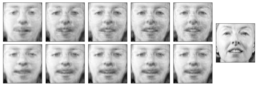
(a)

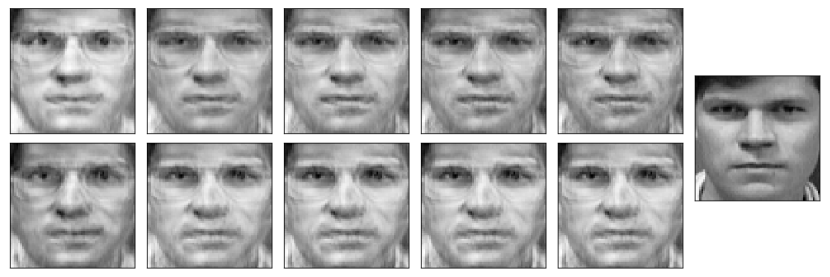
(b)

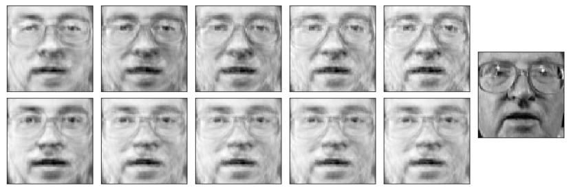
(c)

Figure 2: Reconstruction of test set images. For both (a), (b) and (c): Top: reconstruction by RGCSS. Bottom: reconstruction by GCSS. Right: Original image. We show reconstructions for $k=128,256,512,1024,2048$.

5.6 Running time

In order to evaluate the running time of our algorithm, we generated synthetic matrices of increasing dimensions and ran the algorithms for increasing values of $k$. Figure 3 shows the resulting times for the unregularized (GCSS) and the regularized (RGCSS) algorithms. To measure the sensitivity with respect to each parameter, we fixed the other two. Specifically, we run the following experiments:

• $n=1000,k=128$, $m\in[10^{3},10^{5}]$

• $m=1000,k=1$, $n\in[100,5000]$

• $m=1000,n=1024$, $k\in[10,1020]$

The behavior of both algorithms with respect to $m$ and $n$ (the number of rows and columns respectively) is very similar. For large values of $k$, the regularized variant does exhibit noticeably larger running times. It should be noted, however, that the ratio between the time required by the two algorithms converges to a constant factor. This ratio is shown in the plot for varying values of $k$ to support this claim.

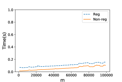
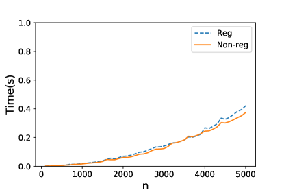
(a)

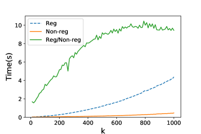
(b)

Figure 3: Running times with respect to the different input parameters. The ratio between the running time of the two algorithms is shown in the plot for the value of $k$.

Table 5: Average pairwise Jaccard index and loss.

	$\bar{J}$
Dataset	$\lambda=0$	$\lambda=1$	$\lambda=10$	$\mathbb{E}[J]$
ORL	0.177	0.245	0.408	0.012
MNIST	0.278	0.951	0.774	0.068
YaleB	0.252	0.632	0.852	0.051
OnlineNews	0.782	1.0	1.0	0.336
Isolet	0.422	0.6	0.838	0.088

6 Conclusions & future work

In this paper we have presented a novel formulation of the Column Subset Selection Problem that incorporates a regularization term. We have derived an efficient algorithm to greedily optimize it, and have demonstrated its potential through various experiments. In addition, we have discussed how this formulation can be inadequate for feature selection and have proposed an alternative that solves this problem. Finally, we have derived a lower bound for the error of the proposed problem. We believe that these new problem formulations open exploration directions with regards to column subset selection. The advantages of using the proposed algorithm in practice have been demostrated by a wide variety of experiments. In future work, it would be interesting to study the impact of the value of $\lambda$ on the generalization ability of the resulting models, and whether significant improvement can be gained by fine-tuning. Additionally, it would be interesting to know whether optimal values can be derived making distributional assumptions with respect to the input data. Finally, it would be interesting to study the possibility of deriving approximation guarantees for the greedy and other algorithms.

Appendix A.

Here we show more detailed derivations of some of the equalities in the paper.

Equality 6:

$$A^{(t+1)}=C_{w}(C_{w}^{T}C_{w}+\lambda I)^{-1}C_{w}^{T}A$$

$$=~{} (C\mbox{ }w)(C_{w}^{T}C_{w}+\lambda I)^{-1}(C\mbox{ }w)^{T}A$$

$$=~{} C(C^{T}C+\lambda I)^{-1}C^{T}A+C\frac{vv^{T}}{\alpha_{w}}C^{T}A-w\frac{v^{T}}{\alpha_{w}}C^{T}A-C\frac{vw^{T}}{\alpha_{w}}A+\frac{ww^{T}}{\alpha_{w}}A$$

$$=~{} A^{(t)}+\frac{(A_{:w}A^{T}_{:w})^{(t)}}{\alpha_{w}}A-w\frac{(A^{T}_{:w})^{(t)}}{\alpha_{w}}A-\frac{A^{(t)}_{:w}w^{T}}{\alpha_{w}}A+\frac{ww^{T}}{\alpha_{w}}A$$

$$=~{} A^{(t)}+\frac{1}{\alpha_{w}}\left((A^{(t)}_{:w}-w)(A^{(t)}_{:w}-w)^{T}\right)A$$

Equality 7:

$$\operatorname*{\arg\!\min}\|A-A^{(t+1)}\|_{F}^{2}$$

$$= \operatorname*{\arg\!\min}_{i}tr\left((A-A^{(t+1)})^{T}(A-A^{(t+1)})\right)$$

$$= \operatorname*{\arg\!\min}_{i}tr(A^{T}A)-tr(A^{T}A^{(t+1)})-tr((A^{T})^{(t+1)}A^{T})+tr((A^{T}A)^{(t+1)})$$

$$= \operatorname*{\arg\!\min}_{i}tr(A^{T}A)-tr(A^{T}(A^{(t)}+\frac{1}{\alpha_{i}}d_{i}d_{i}^{T}A))$$

$$-tr((A^{(t)}+\frac{1}{\alpha_{i}}d_{i}d_{i}^{T}A)^{T}A)+tr((A^{(t)}+\frac{1}{\alpha_{i}}d_{i}d_{i}^{T}A)^{T}(A^{(t)}+\frac{1}{\alpha_{i}}d_{i}d_{i}^{T}A))$$

$$= \operatorname*{\arg\!\min}_{i}tr(A^{T}A)-tr(A^{T}A^{(t)})-tr(\frac{1}{\alpha_{i}}A^{T}d_{i}d_{i}^{T}A))$$

$$-tr((A^{T})^{(t)}A)-tr(\frac{1}{\alpha_{i}}A^{T}d_{i}d_{i}^{T}A)$$

$$+tr((A^{T})^{(t)}A^{(t)})+tr(\frac{1}{\alpha_{i}}(A^{T})^{(t)}d_{i}d_{i}^{T}A)+tr(\frac{1}{\alpha_{i}}A^{T}d_{i}d_{i}^{T}A^{(t)})$$

$$+tr(\frac{1}{\alpha_{i}^{2}}A^{T}d_{i}d_{i}^{T}d_{i}d_{i}^{T}A)$$

Equality 8:

$$\operatorname*{\arg\!\min}\|A-A^{(t+1)}\|_{F}^{2}$$

$$= -2tr(\frac{1}{\alpha_{i}}A^{T}d_{i}d_{i}^{T}A)+2tr(\frac{1}{\alpha_{i}}(A^{T})^{(t)}d_{i}d_{i}^{T}A)+tr(\frac{1}{\alpha_{i}^{2}}A^{T}d_{i}d_{i}^{T}d_{i}d_{i}^{T}A)$$

$$= \operatorname*{\arg\!\min}_{i}\frac{2}{\alpha_{i}}tr((A^{T})^{(t)}d_{i}d_{i}^{T}A)-\frac{2}{\alpha_{i}}tr(A^{T}d_{i}d_{i}^{T}A)+\frac{1}{\alpha_{i}^{2}}\|d_{i}d_{i}^{T}A\|_{F}^{2}$$

$$= \operatorname*{\arg\!\min}_{i}\frac{2}{\alpha_{i}}\tilde{x}_{i}^{T}x_{i}-\frac{2}{\alpha_{i}}\|x_{i}\|_{2}^{2}+\frac{1}{\alpha_{i}^{2}}\|d_{i}\|_{2}^{2}\|x_{i}\|_{2}^{2}$$

$$= \operatorname*{\arg\!\min}_{i}\frac{2}{\alpha_{i}}(\tilde{x}_{i}-x_{i})^{T}x_{i}+\frac{1}{\alpha_{i}^{2}}\|x_{i}\|_{2}^{2}(\tilde{x}_{ii}-x_{ii})$$

$$= \operatorname*{\arg\!\min}_{i}\frac{2}{\alpha_{i}}\tilde{x}_{i}^{T}x_{i}+(\frac{-2}{\alpha_{i}}+\frac{1}{\alpha_{i}^{2}}(\tilde{x}_{ii}-x_{ii}))x_{i}^{T}x_{i}+\lambda$$

Equality 9

$$A^{T}A^{(t+1)}= A^{T}(A^{(t)}+\frac{1}{\alpha_{w}}d_{w}d_{w}^{T}A)$$

$$= A^{T}A^{(t)}+\frac{1}{\alpha_{w}}A^{T}d_{w}d_{w}^{T}A$$

$$= A^{T}A^{(t)}+\frac{1}{\alpha_{w}}x_{w}x_{w}^{T}$$

Equality 10

$$(A^{T}A)^{(t+1)}= (A^{(t)}+\frac{1}{\alpha_{w}}d_{w}d_{w}^{T}A)^{T}(A^{(t)}+\frac{1}{\alpha_{w}}d_{w}d_{w}^{T}A)$$

$$= (A^{T}A)^{(t)}+\frac{1}{\alpha_{w}}(A^{T})^{(t)}d_{w}d_{w}^{T}A+\frac{1}{\alpha_{w}}A^{T}d_{w}d_{w}^{T}A^{(t)}+\frac{1}{\alpha_{w}^{2}}A^{T}d_{w}d_{w}^{T}d_{w}d_{w}^{T}A$$

$$= (A^{T}A)^{(t)}+\frac{1}{\alpha_{w}}\tilde{x}_{w}x_{w}^{T}+\frac{1}{\alpha_{w}}x_{w}\tilde{x}_{w}^{T}+\frac{1}{\alpha_{w}^{2}}x_{w}d_{w}^{T}d_{w}x_{w}^{T}$$

Equality 11

$$X^{(t+1)} =A^{T}D^{(t+1)}$$

$$=A^{T}A^{(t+1)}-A^{T}A$$

$$=A^{T}A^{(t)}+\frac{1}{\alpha_{w}}x_{w}x_{w}^{T}-A^{T}A$$

$$=A^{T}D^{(t)}+A^{T}A+\frac{1}{\alpha_{w}}x_{w}x_{w}^{T}-A^{T}A$$

$$=X^{(t)}+\frac{1}{\alpha_{w}}x_{w}x_{w}^{T}=X^{(0)}+\sum_{i=0}^{t}\left(\frac{1}{a_{w}}x_{w}x_{w}^{T}\right)^{(i)}$$

Equality 12

$$\tilde{X}^{(t+1)} =(A^{T}D)^{(t+1)}$$

$$=(A^{T}A)^{(t+1)}-(A^{T})^{(t+1)}A$$

$$=(A^{T}A)^{(t)}+\frac{1}{\alpha_{w}}\tilde{x}_{w}x_{w}^{T}+\frac{1}{\alpha_{w}}x_{w}\tilde{x}_{w}^{T}+\frac{1}{\alpha_{w}^{2}}x_{w}d_{w}^{T}d_{w}x_{w}^{T}-(A^{T})^{(t)}A-\frac{1}{\alpha_{w}}x_{w}x_{w}^{T}$$

$$=(A^{T}A)^{(t)}-(A^{T})^{(t)}A+\frac{1}{\alpha_{w}}\tilde{x}_{w}x_{w}^{T}+\frac{1}{\alpha_{w}}x_{w}\tilde{x}_{w}^{T}+\frac{1}{\alpha_{w}^{2}}x_{w}d_{w}^{T}d_{w}x_{w}^{T}-\frac{1}{\alpha_{w}}x_{w}x_{w}^{T}$$

$$=(A^{T}D)^{(t)}+\frac{1}{\alpha_{w}}\tilde{x}_{w}x_{w}^{T}+\frac{1}{\alpha_{w}}x_{w}\tilde{x}_{w}^{T}+\frac{1}{\alpha_{w}^{2}}x_{w}d_{w}^{T}d_{w}x_{w}^{T}-\frac{1}{\alpha_{w}}x_{w}x_{w}^{T}$$

$$=X^{(0)}+\sum_{i=0}^{t}\left(\frac{1}{\alpha_{w}}\tilde{x}_{w}x_{w}^{T}+\frac{1}{\alpha_{w}}x_{w}\tilde{x}_{w}^{T}+\frac{1}{\alpha_{w}^{2}}x_{w}d_{w}^{T}d_{w}x_{w}^{T}-\frac{1}{\alpha_{w}}x_{w}x_{w}^{T}\right)^{(i)}$$

Declarations of interest: none.

References

- [1] A. Çivril, Column subset selection problem is ug-hard, Journal of Computer and System Sciences 80 (4) (2014) 849–859.
- [2] Y. Shitov, Column subset selection is np-complete, arXiv preprint arXiv:1701.02764.
- [3] J. Altschuler, A. Bhaskara, G. Fu, V. Mirrokni, A. Rostamizadeh, M. Zadimoghaddam, Greedy column subset selection: New bounds and distributed algorithms, in: International Conference on Machine Learning, 2016, pp. 2539–2548.
- [4] A. K. Farahat, A. Ghodsi, M. S. Kamel, An efficient greedy method for unsupervised feature selection, in: Data Mining (ICDM), 2011 IEEE 11th International Conference on, IEEE, 2011, pp. 161–170.
- [5] X. He, D. Cai, P. Niyogi, Laplacian score for feature selection, in: Advances in neural information processing systems, 2005, pp. 507–514.
- [6] Z. Zhao, H. Liu, Spectral feature selection for supervised and unsupervised learning, in: Proceedings of the 24th international conference on Machine learning, ACM, 2007, pp. 1151–1157.
- [7] Z. Xu, I. King, M. R.-T. Lyu, R. Jin, Discriminative semi-supervised feature selection via manifold regularization, IEEE Transactions on Neural networks 21 (7) (2010) 1033–1047.
- [8] D. Cai, C. Zhang, X. He, Unsupervised feature selection for multi-cluster data, in: Proceedings of the 16th ACM SIGKDD international conference on Knowledge discovery and data mining, ACM, 2010, pp. 333–342.
- [9] Z. Zhao, L. Wang, H. Liu, et al., Efficient spectral feature selection with minimum redundancy., in: AAAI, 2010, pp. 673–678.
- [10] Y. Yang, H. T. Shen, Z. Ma, Z. Huang, X. Zhou, l2, 1-norm regularized discriminative feature selection for unsupervised learning, in: IJCAI proceedings-international joint conference on artificial intelligence, Vol. 22, 2011, p. 1589.
- [11] Z. Li, Y. Yang, J. Liu, X. Zhou, H. Lu, et al., Unsupervised feature selection using nonnegative spectral analysis., in: AAAI, Vol. 2012, 2012, pp. 1026–1032.
- [12] Z. Zhao, L. Wang, H. Liu, J. Ye, On similarity preserving feature selection, IEEE Transactions on Knowledge and Data Engineering 25 (3) (2013) 619–632.
- [13] C. Hou, F. Nie, D. Yi, Y. Wu, Feature selection via joint embedding learning and sparse regression, in: IJCAI Proceedings-International Joint Conference on Artificial Intelligence, Vol. 22, 2011, p. 1324.
- [14] R. He, T. Tan, L. Wang, W.-S. Zheng, l 2, 1 regularized correntropy for robust feature selection, in: Computer Vision and Pattern Recognition (CVPR), 2012 IEEE Conference on, IEEE, 2012, pp. 2504–2511.
- [15] M. Qian, C. Zhai, Robust unsupervised feature selection., in: IJCAI, 2013, pp. 1621–1627.
- [16] C. Hou, F. Nie, X. Li, D. Yi, Y. Wu, Joint embedding learning and sparse regression: A framework for unsupervised feature selection, IEEE Transactions on Cybernetics 44 (6) (2014) 793–804.
- [17] S. Wang, J. Tang, H. Liu, Embedded unsupervised feature selection., in: AAAI, 2015, pp. 470–476.
- [18] L. Du, Y.-D. Shen, Unsupervised feature selection with adaptive structure learning, in: Proceedings of the 21th ACM SIGKDD International Conference on Knowledge Discovery and Data Mining, ACM, 2015, pp. 209–218.
- [19] S. Wang, W. Pedrycz, Q. Zhu, W. Zhu, Unsupervised feature selection via maximum projection and minimum redundancy, Knowledge-Based Systems 75 (2015) 19–29.
- [20] T. F. Chan, Rank revealing qr factorizations, Linear algebra and its applications 88.
- [21] A. Frieze, R. Kannan, S. Vempala, Fast monte-carlo algorithms for finding low-rank approximations, Journal of the ACM (JACM) 51 (6) (2004) 1025–1041.
- [22] M. W. Mahoney, P. Drineas, Cur matrix decompositions for improved data analysis, Proceedings of the National Academy of Sciences 106 (3) (2009) 697–702.
- [23] C. Boutsidis, M. W. Mahoney, P. Drineas, An improved approximation algorithm for the column subset selection problem, in: Proc. of the 20th Annual ACM-SIAM Symp. on Discrete Algorithms, Soc. for Industrial and Applied Mathematics, 2009, pp. 968–977.
- [24] C. Boutsidis, P. Drineas, M. Magdon-Ismail, Near-optimal column-based matrix reconstruction, SIAM Journal on Computing 43 (2) (2014) 687–717.
- [25] A. Civril, M. Magdon-Ismail, Column subset selection via sparse approximation of svd, Theoretical Computer Science 421 (2012) 1–14.
- [26] B. Ordozgoiti, S. G. Canaval, A. Mozo, A fast iterative algorithm for improved unsupervised feature selection, in: Data Mining (ICDM), 2016 IEEE 16th International Conference on, IEEE, 2016, pp. 390–399.
- [27] B. Ordozgoiti, S. G. Canaval, A. Mozo, Iterative column subset selection, Knowledge and Information Systems (2017) 1–30.
- [28] H. Lutkepohl, Handbook of matrices., Computational Statistics and Data Analysis 2 (25) (1997) 243.
- [29] R. C. Thompson, Principal submatrices ix: Interlacing inequalities for singular values of submatrices, Linear Algebra and its Applications 5 (1) (1972) 1–12.
- [30] M. Fanty, R. Cole, Spoken letter recognition, in: Advances in Neural Information Processing Systems, 1991, pp. 220–226.
- [31] Y. LeCun, C. Cortes, C. J. Burges, Mnist handwritten digit database, AT&T Labs [Online]. Available: http://yann. lecun. com/exdb/mnist 2.
- [32] A. S. Georghiades, P. N. Belhumeur, D. J. Kriegman, From few to many: Illumination cone models for face recognition under variable lighting and pose, Pattern Analysis and Machine Intelligence, IEEE Transactions on 23 (6) (2001) 643–660.
- [33] F. S. Samaria, A. C. Harter, Parameterisation of a stochastic model for human face identification, in: Applications of Computer Vision, 1994., Proceedings of the Second IEEE Workshop on, IEEE, 1994, pp. 138–142.
- [34] S. A. Nene, S. K. Nayar, H. Murase, Columbia object image library (coil-20), Tech. Rep. CUCS-005-96, Columbia University (February 1996).
- [35] K. Fernandes, P. Vinagre, P. Cortez, A proactive intelligent decision support system for predicting the popularity of online news, in: Progress in Artificial Intelligence, Springer, 2015, pp. 535–546.