Unsupervised Discovery of Object Landmarks as Structural Representations
Abstract
Deep neural networks can model images with rich latent representations, but they cannot naturally conceptualize structures of object categories in a human-perceptible way. This paper addresses the problem of learning object structures in an image modeling process without supervision. We propose an autoencoding formulation to discover landmarks as explicit structural representations. The encoding module outputs landmark coordinates, whose validity is ensured by constraints that reflect the necessary properties for landmarks. The decoding module takes the landmarks as a part of the learnable input representations in an end-to-end differentiable framework. Our discovered landmarks are semantically meaningful and more predictive of manually annotated landmarks than those discovered by previous methods. The coordinates of our landmarks are also complementary features to pretrained deep-neural-network representations in recognizing visual attributes. In addition, the proposed method naturally creates an unsupervised, perceptible interface to manipulate object shapes and decode images with controllable structures. The project web page: http://ytzhang.net/projects/lmdis-rep
.tocmtchapter \etocsettagdepthmtchaptersubsection \etocsettagdepthmtappendixnone
1 Introduction
Computer vision seeks to understand object structures that reflect the physical states of objects and show invariance to individual appearance changes. Such intrinsic structures can serve as intermediate representations for high-level visual understanding. However, manual annotations or designs of object structures (e.g., skeleton, semantic parts) are costly and barely available for most object categories, making the automatic representation learning of object structure an attractive solution to this challenge.
Modern neural networks can learn latent representations to effectively solve various vision problems, including image classification [26, 53, 56, 20], segmentation [32, 40, 21], object detection [17, 80, 49], human pose estimation [39], 3D reconstruction [13, 67, 14], and image generation [25, 18, 43]. Several existing studies [17, 76, 1] observe that these representations naturally encode massive templates of particular visual patterns. However, little evidence suggests that deep neural networks can naturally conceptualize the intrinsic structures of an object category compactly and perceptibly.
We aim at learning the physical parameters of conceptualized object structures without supervision. As a typical representation of intrinsic structures, landmarks represent the spatial configuration of stable local semantics across different object instances of the same category. Thewlis et al. [59] proposed an unsupervised method to locate landmarks at the places where a convolutional neural network can detect stable visual patterns with high spatial equivariance to image transformations. However, this method did not explicitly encourage the landmarks to appear at critical locations for image modeling.
This paper addresses the problem of discovering landmarks in a generic image modeling process. In particular, we take landmark discovery as an intermediate step for image autoencoding. To leverage the training signals from the landmark-based image decoder, gradients need to go through the landmark coordinates, which makes Thewlis et al. [59]’s non-differentiable formulation infeasible. With a different way to calculate landmark coordinates, the image decoding module can make the landmark configuration informative regarding image reconstruction. We also introduce additional regularization terms to enforce the desirable properties of the detected landmarks and to prevent the landmark coordinates from encoding irrelevant or redundant latent information.
Our contributions in this paper are as follows.
-
1.
We develop a differentiable autoencoder framework for object landmark discovery, which allows the image decoder to propagate training signals back to the landmark detection module. We introduce several soft constraints to reflect the properties of landmarks, forcing the discovered representations to be valid landmarks.
-
2.
The proposed method discovers visually meaningful landmarks without supervision for a variety of objects. It outperforms the state-of-the-art method regarding the accuracy of predicting manually-annotated landmarks using discovered landmarks, and it performs comparably to fully supervised landmark detectors trained with a significant amount of labeled data.
-
3.
The discovered landmarks show strong discriminative performance in recognizing visual attributes.
-
4.
Our landmark-based image decoder is useful for controllable image decoding, such as object shape manipulation and structure-conditioned image generation.
2 Related work
Discriminative part learning.
Parts are commonly used object structures in computer vision. The deformable part-based model [15] learns object part configurations to optimize the object detection accuracy, where similar ideas are rooted in earlier constellation approaches [16, 66, 6]. A recent method [72] based on the deep neural network performs end-to-end learning of deformable mixture of parts for pose estimation. The recurrent architecture [19] and spatial transformer network [23] are also used to discover and refine object parts for fine-grained image classification [27]. In addition, discriminative mid-level patches can be also discovered without explicit supervision [54]. Object-part discovery based on subspace analysis and clustering techniques is also shown to improve neural-network-based image recognition [52]. Unlike the approaches specific to discriminative tasks, our work focuses on learning landmarks for generic image modeling.
Learning structural representations.
To capture the intrinsic structures of objects, existing studies [44, 45, 37] disentangle visual content into multiple factors of variations, like the camera viewpoint, motion, and identity. The physical parameters of these factors are, however, still embedded in non-perceptible latent representations. Methods based on multi-task learning [78, 21, 65, 81] can take conceptualized structures (e.g., landmarks, masks, depth) as additional outputs. These structures in this setting are designed by humans and require supervision to learn.
Learning explicit structures for image correspondence.
Object structures create correspondence among object instances. Colocalization [57, 9] realizes the coarsest level of object correspondence. In a finer granularity, AnchorNet [41] learns object parts and their correspondence across different objects and categories. WarpNet [24] corresponds images in the same class by estimating the parameter of a thin plate spline (TPS) transformation [4], and it can roughly reconstruct 3D point cloud using a single-view image. The 3D interpreter network [67] utilizes 2D landmark annotations to discover 3D skeletons as the explicit structures of objects. Our discovered landmarks are denser than object parts and sparser than 3D points. These landmark representations are also more sensitive to precise locations and obtained without supervision.
Landmark discovery with equivariance.
Object structures like landmarks should be equivariant to image transformation, including object and camera motions. Using this property in 2D image domain, Rocco et al. [50] proposed to discover TPS control points to match pairs of object images densely. Thewlis et al. [58] tried to densely map different objects to a canonical coordinate that reflects object structures. Instead of learning dense correspondence, Thewlis et al. [59] took the same equivariance property as the guidance to train deep neural networks for object landmark discovery without manual supervision. A similar idea was formulated differently using hand-crafted features in early work [30]. In comparison, our method not only takes the equivariance as a constraint to ensure the validity of the landmarks, but also use a differentiable formulation to incorporate the landmark coordinates into a generic image modeling process. Moreover, our discovered landmarks are more predictive of manually annotated landmarks than those obtained by Thewlis et al. [59], and our method works on a broader range of object categories.
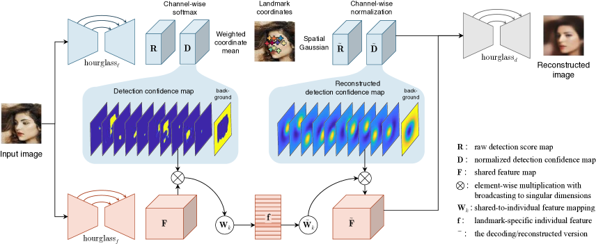
Image modeling with landmarks.
Many unsupervised deep learning techniques exist to model visual content, including stacked autoencoders (SAE) [2, 36], variational autoencoders [25], generative adversarial networks (GAN) [18, 43], and auto-regressive networks [63] (e.g., PixelCNN [62]). The GAN- and PixelCNN-based image generators conditioned on given object landmarks are proposed in [46, 47]. In contrast, our method uses the SAE framework to automatically discover landmarks that are informative for unsupervised image modeling.
Landmark detection.
A vast amount of supervised landmark detection methods exist in the literature. For human faces, there are active appearance models [10, 38, 11], template-based methods [42, 83], regression-based methods [61, 12, 7, 48], and more recent methods based on deep neural networks [55, 77, 81, 82, 75, 70, 68, 33, 71]. Landmark detection methods are also available for human bodies [73, 60, 39], and birds [75]. We use our discovered landmarks to predict manually annotated landmarks and compare our method with some recent supervised models.
3 Autoencoding-based landmark discovery
We aim at automatically discovering landmarks as an explicit representation of visual content. We propose an autoencoder that encodes landmark coordinates as (a part of) the encoder outputs (Section 3.1). Without supervision from hand-crafted labels, we introduce several constraints to encourage the discovered landmark coordinates to reflect the visual concept that agrees with human perception (Section 3.2). The proposed constraints prevent landmark-based representations from degenerating to non-perceptible latent representations. Another pathway of the encoder extracts the local latent descriptor for each discovered landmark (Section 3.3). We use both the landmarks and the latent descriptors to reconstruct the input image (Section 3.4). This section presents the fully differentiable neural network architecture (Figure 1) and training objectives (Section 3.5) for landmark discovery and unsupervised image modeling.
3.1 Architecture of landmark detector
We formulate landmark localization as the problem of detecting particular keypoints in the image [39]. Specifically, each landmark has a corresponding detector, which convolutionally outputs a detection score map with the detected landmark located at the maximum. In this framework, we use a deep neural network to transform an image to a -channel detection confidence map . This map detects landmarks, and the -th channel represents background. ’s resolution can be either equal to or less than that of , but they should have the same aspect ratio. Inspired by the success of the stacked hourglass network in human pose estimation [39], we propose a light-weighted hourglass-style network to get the raw detection score map
| (1) |
where denotes the parameters. The hourglass-style architecture (Appendix G.2) allows detectors to focus on the critical local patterns at landmark locations while utilizing higher-level context. Then, we transform the unbounded raw scores to probabilities and encourage each channel to detect a different pattern. To this end, we normalize across the channels (including the background) using softmax and obtain the detection confidence map
| (2) |
where the matrix is the -th channel of , and the scalar is the value of at the pixel . Later, we also use the vector to denote the multi-channel values of at . The same notation convention applies to other tensors of three axes.
Taking as a weighting map, we use the weighted mean coordinate as the location of the -th landmark, i.e.,
| (3) |
where is the spatial normalization factor. This formulation enables back-propagating the gradient from the downstream neural network through the landmark coordinates unless ’s mass is totally concentrated in a single pixel or totally uniformly distributed, which rarely happens in practice. As a shorthand notation, we write the landmarks and landmark detector as
| (4) |
The left half of the blue pathway in Figure 1 illustrates the landmark detector.
3.2 Visual concept of landmarks
The elements in are supposed to be the discovered landmark coordinates, but so far, there is no guarantee to prevent them from being arbitrary latent representations. Therefore, we propose the following soft constraints as regularizers to enforce the desirable properties for landmarks.
Concentration constraint
As a detection confidence map for a single location, the mass of need to be concentrated in a local region. Taking (spatially normalized as in (3)) as the density of a bivariate distribution on the image coordinate, we compute its variance and along the two axes. We define the concentration constraint loss as follows to encourage both variances to be small:
| (5) |
This equation makes the exponential of the entropy of the isotropic Gaussian distribution , where , and is the identity matrix. This Gaussian distribution is an approximation of , and lower entropy means a more peaked distribution. Note that, formally, this approximation is
| (6) |
Separation constraint
Ideally, the autoencoder training objective can automatically encourage the landmarks to be distributed at different local regions so that the whole image can be reconstructed. However, the initial randomness can make the landmarks, defined as the mean coordinates weighted by as in (3), all around the image center in the beginning of the training. This can lead to local optima from which the gradient descent may not escape (see Appendix F.2). To circumvent this difficulty, we introduce an explicit loss to spatially separate the landmarks:
| (7) |
Equivariance constraint
A landmark should locate a stable local pattern (with definite semantics). This requires landmarks to show equivariance to image transformations. More specifically, a landmark should move according to the transformation (e.g., camera and object motion) applied to the image if the corresponding visual semantics still exist in the transformed image. Let be a coordinate transformation that map image to , and . We ideally have , inducing the soft constraint
| (8) |
This loss function is well-defined when is known. Inspired by Thewlis et al. [59], we simulate by a thin plate spline (TPS) [4] with random parameters. We use random translation, rotation, and scaling to determine the global affine component of the TPS; and, we spatially perturb a set of control points to determine the local TPS component. Besides the conventional way of selecting TPS control points at a predefined uniform grid (as used in [59]), we also take the landmarks detected by the current model as the control points to improve simulated transformation’s focus on key image patterns. The two sets of control points are alternatively used in each optimization iteration (see Appendix F.3 for details). Moreover, when training sample appear in the form of video, we can also take the dense motion flow as and the actual next frame as .
Cross-object correspondence
Our model does not explicitly ensure the semantic correspondence among the landmarks discovered on different object instances. The cross-object semantic stability of the landmarks mainly relies on the fact that visual patterns activating the same convolutional filter are likely to share semantic similarities.
3.3 Local latent descriptors
For simple images, like in MNIST [29] (see results for MNIST in Appendix B), multiple landmarks can be enough to describe the object shapes. For most natural images, however, landmarks are insufficient to represent all visual content, so extra latent representations are needed to encode complementary information. Though necessary, the latent representations should not encode too much holistic information that can overwhelm the image structures reflected by the landmarks. Otherwise, the autoencoder would not provide enough driving force to localize landmarks at meaningful locations. To achieve this trade-off, we attach a low-dimensional local descriptor to each landmark.
An hourglass-style neural network (see Appendix G.2) is introduced to obtain a feature map , which has the same size as the detection confidence map :
| (9) |
Note that is in a feature space shared among all landmarks and has channels.
For each landmark, we use an average pooling weighted by a soft mask centered at the landmark to extract the local feature in the shared space. In particular, we take , which is the Gaussian approximation of the detection confidence map defined in (6), as the soft mask. Then, a learnable linear operator is introduced for each landmarks to map the feature representation into a lower-dimensional individual space. Thus, the latent descriptor for the -th landmark is
| (10) |
where . The landmark-specific linear operator enables each landmark descriptor to encode a particular pattern in limited bits. We can also use (10) to extract a low-dimensional background descriptor. Since it is unreasonable to approximate the background confidence map with a Gaussian distribution, we exactly set . Note that is differentiable regarding both the feature map and the detection confidence map.
Putting all latent descriptors together, we have . The left half of the red pathway in Figure 1 illustrates the neural network architecture to extract the landmark descriptors.
3.4 Landmark-based decoder
We approximately invert the landmark coordinates to the detection confidence map . Concretely, we use the probability density of an isotropic Gaussian distribution centered at each landmark to get raw score maps
| (11) |
and the background channel is set to . is then normalized across channels to obtain the reconstructed detection confidence map
| (12) |
Figure 1 (right half of the blue pathway) illustrates this.
For each landmark (including the background) descriptor , we transform it into a shared feature space by the landmark-specific operator and an activation function (e.g., LeakyReLU [34]). Using as the soft switches for global unpooling, we recover the feature map
| (13) |
where is the non-linear activation function. This is illustrated by the right half of the red pathway in Figure 1.
Though alternative neural network architectures are available (e.g., in [46, 47]) for landmark-conditioned image decoding, our proposed architecture enables back-propagation through the landmark coordinates. The Gaussian variance determines how much the neighboring pixels can contribute to the gradients for the landmark coordinates and how sharp the descriptor is localized in the recovered feature map. While it is important to include more pixels for back-propagation in the early stage of training, sharpness becomes more important as training goes on. To balance the two needs, we obtain multiple versions of under different values of , say, .
Let be the channel-wise concatenation. We use another hourglass-style network to reconstruct the image
| (14) |
The gray pathway in Figure 1 illustrates the image decoder.
3.5 Overall training objective
The image reconstruction loss drives the training of the entire autoencoder. We define as , and is normalized to . The full loss is
| (15) |
4 Experiments
We evaluate our method on a variety of datasets, including CelebA [31] and AFLW [35] for human faces, the cat head dataset [79], a car dataset built from PASCAL 3D [69], shoe images from UT Zappos50k [74], human pose images from Human3.6M [22, 8], MNIST (Appendix B), and animal images from AwA [28] (Appendix D).
Section 4.1 describes the datasets and shows the qualitative results of landmark discovery. In Section 4.2, we use the discovered landmarks to predict human-annotated landmarks, and we take the landmark detection accuracy as an indicator of the quality of discovered landmark. Section 4.3 demonstrates that our discovered landmarks can serve as effective image representations to predict shape-related facial attributes on CelebA. In Section 4.3, we show that our decoding module and the automatically discovered landmarks can be used to manipulate the object shapes.
4.1 Landmark discovery on multiple datasets
We train and evaluate landmark discovery models on a variety of objects. The detailed architectures of the neural network modules (i.e., ) depend on the image sizes on different datasets. Appendix G describes implementation details, including data preprocessing, network architectures, model parameters, and optimization methods.


CelebA
Following [59], we use all facial images in the CelebA training set excluding those also appearing in the MAFL the test set111The MAFL dataset [81] is a subset of CelebA. (then 16,1962 images in total) to train models for landmark discovery. We use the MAFL testing set (1000 images) for all testing cases and reserve the MAFL training set (19,000 images) to train prediction models for manually-annotated landmarks. By default, we use the cropped and aligned images provided in the dataset.
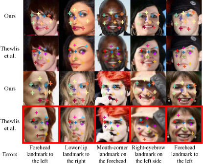
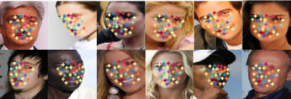
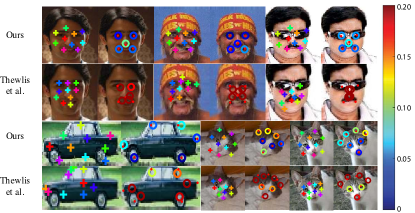
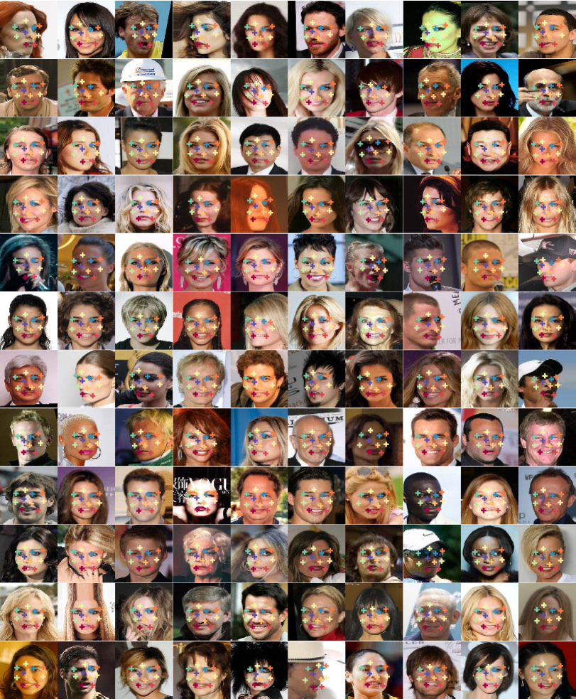
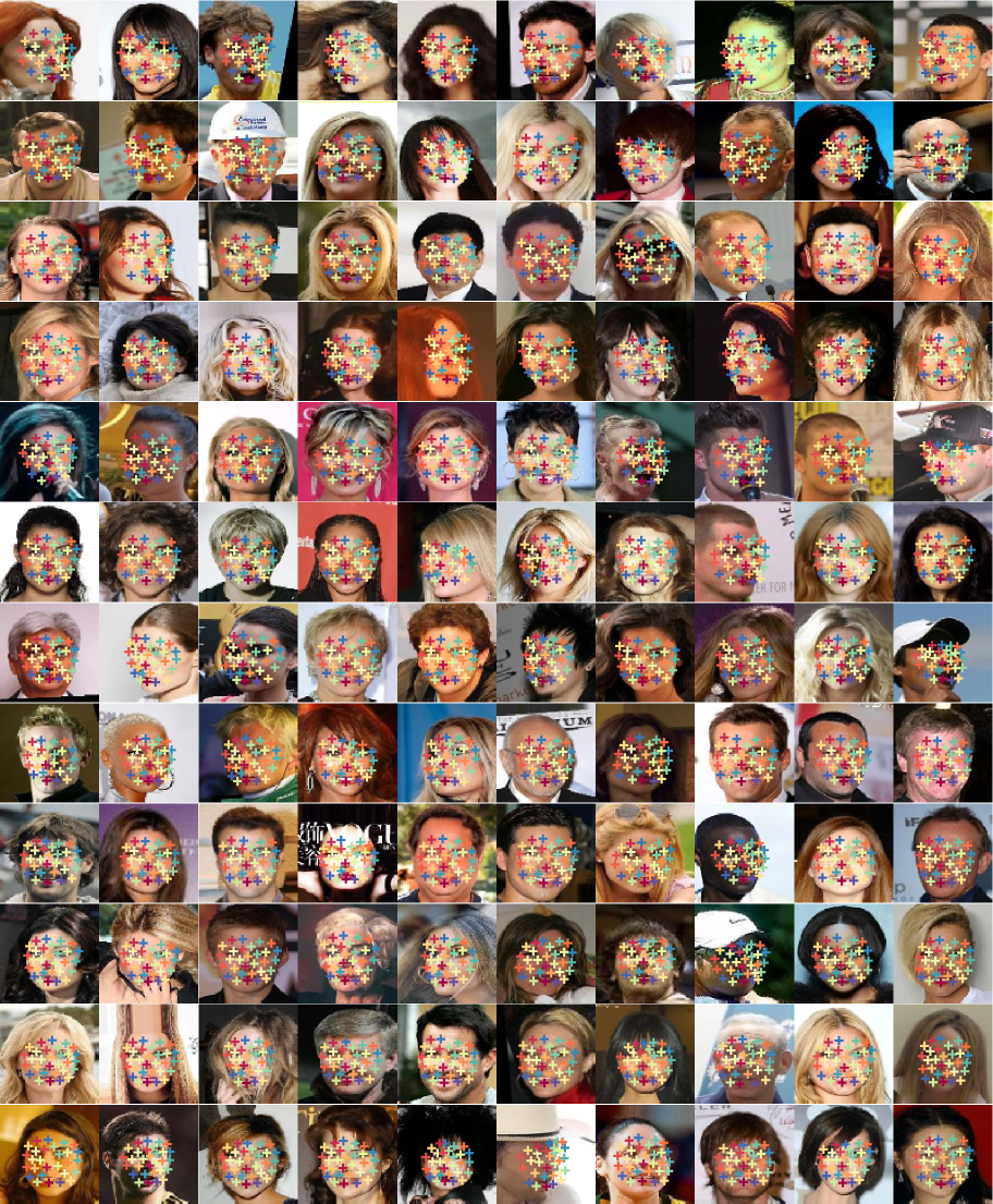
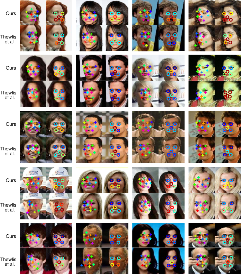
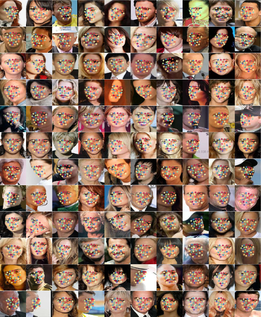
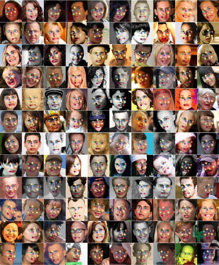
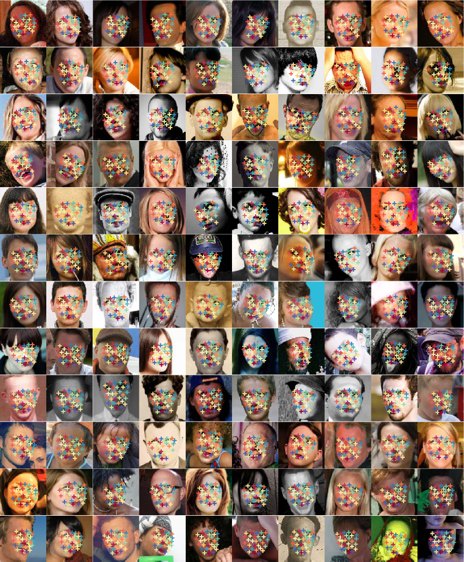
As shown in Figure 2, our method can automatically discover facial landmarks at semantically meaningful and stable locations, such as the forehead center, eyes, eyebrows, nose, and mouth corners. Compared to Thewlis et al. [59]’s method, which results in a few significant errors, our method can locate landmarks more robustly against pose variations and occlusions. Interestingly, our method can work out-of-the-box on head-shoulder portraits without training on exactly the same type of images (Figure 3). Figure 4 shows that our method can also learn and detect a larger number (e.g., 30) of high-quality landmarks on unaligned facial images. Appendix E.1 shows more results.
AFLW
Face images in AFLW are cropped differently from CelebA. The landmark discovery models (both ours and Thewlis et al. [59]’s) are pretrained on CelebA and finetuned on the AFLW training set (10,122 images) for adaptation. Sampled results on the AFLW testing set (2,991 images) are in Appendix E.2.

Cat heads
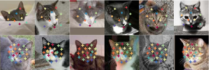
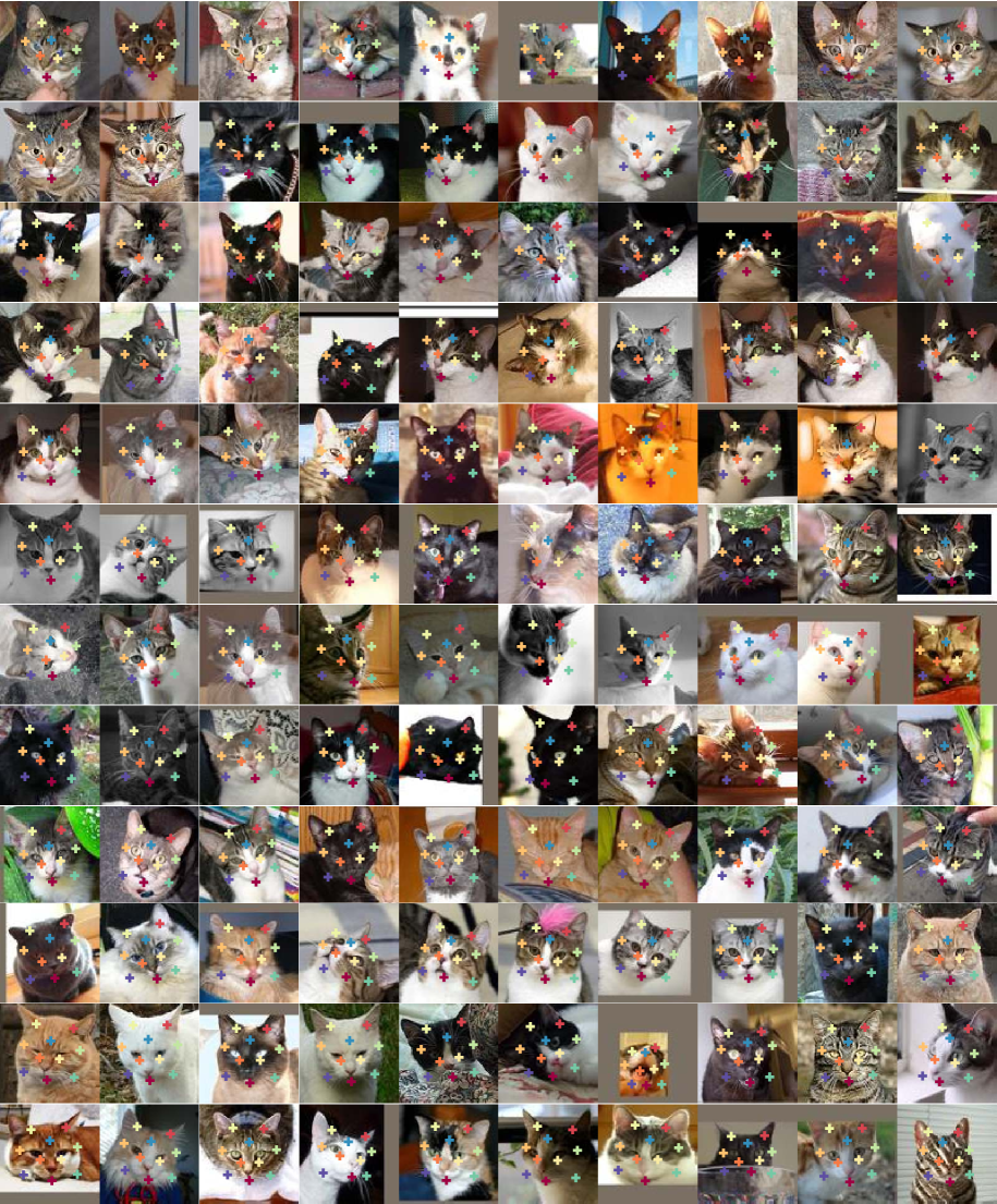
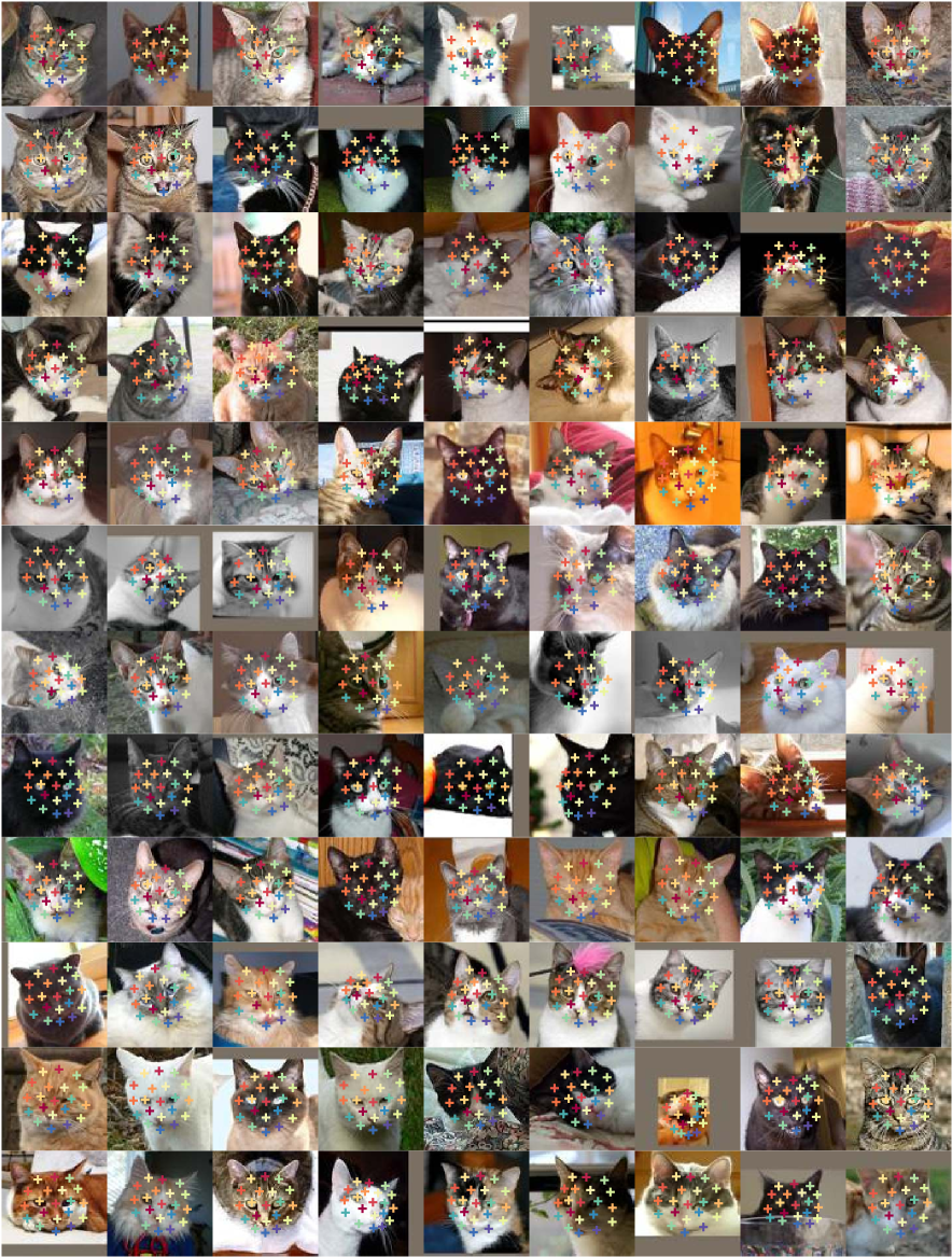
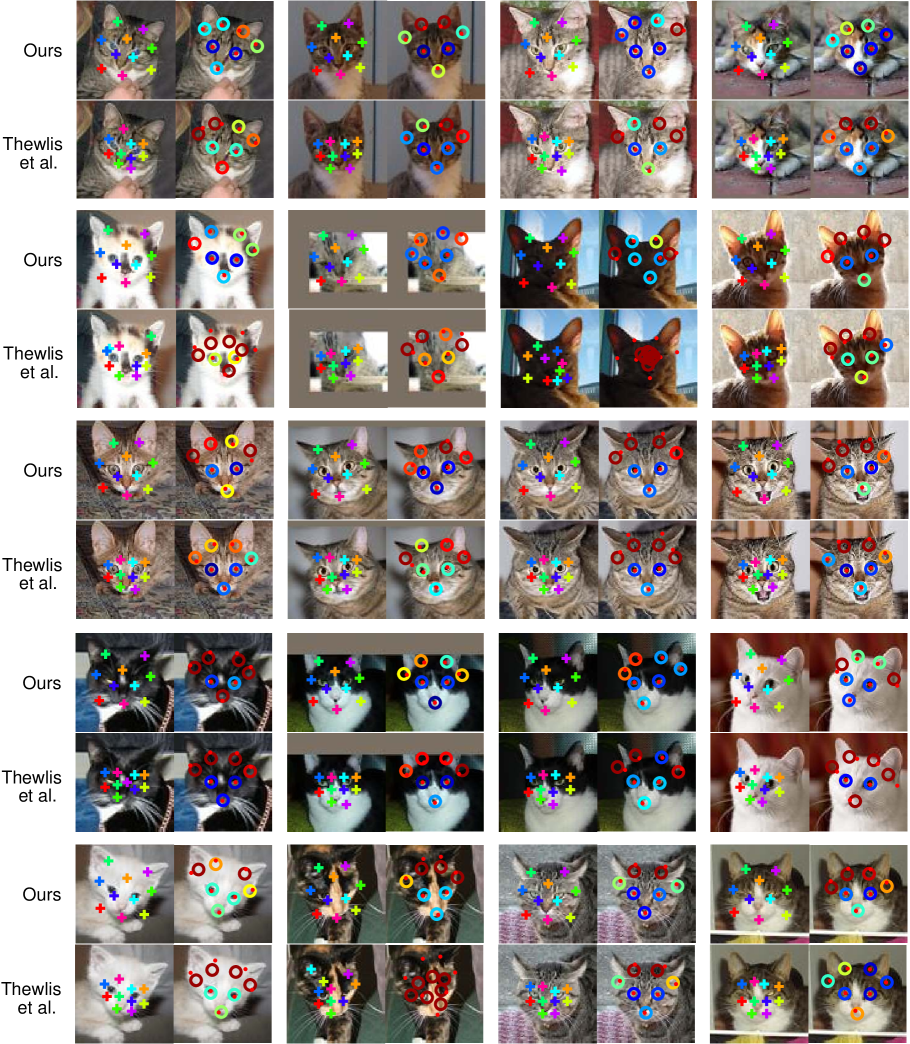
Our model is trained on 7,747 cat head images and tested on 1,257 images. Compared to human faces, cat heads show more holistic appearance variations. As shown in Figure 5, our model can discover consistent landmarks (e.g., ears, nose, mouth) across different cat species and interestingly predict landmark locations under significant occlusion (the first image). Appendix E.3 shows more results.
Cars
We build the profile-view car dataset by cropping the car images from the PASCAL 3D dataset. This dataset has a limited number of samples (567 images for training and 63 images for testing). As shown in Figure 7, our method can still learn meaningful landmarks (e.g., the windshield, driver-side door, wheels, rear) using a relatively small training set. Note that we transform the 3D annotations of the cars to 2D landmarks, so this dataset is ready for quantitative evaluation. Appendix E.4 shows more results.
Shoes
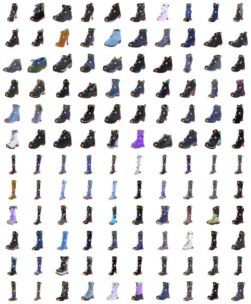
We use the same setting as in [59] (49,525, training images and 500 testing images). As shown in Figure 6, landmarks are detected at semantically stable locations for different types of shoes. Appendix E.5 shows more results.

Human3.6M
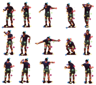
Human3.6M contains human activity videos in stable backgrounds. We use all 7 subjects in Human3.6M training set for our evaluation (6 for training and 1 for validation)222Training subject IDs: S1,S5,S6,S7,S8,S9; Validation subject IDs: S11.. We consider six activities (direction, discussion, posing, waiting, greeting, walking), in which human bodies are in the upright direction most of the time, resulting in 796,648 image frames for training and 87,975 image frames for testing. We removed the background using the off-the-shelf unsupervised background subtraction method provided in the dataset. The human bodies are cropped and roughly aligned regarding the foot location so that the excessive background regions are removed.
Compared to previously mentioned object types, human bodies have much more shape variations. As shown in Figure 8, our method can discover roughly consistent landmarks across a range of poses. In particular, the landmarks at the head, back, waist, and legs are stable across images. The landmarks at the arms are relatively less consistent across different poses, but they are still at semantically meaningful locations. Since the human body appearances in the frontal and back views are similar, we do not expect our discovered landmarks to distinguish the left and right sides of the human body, which means that a landmark at the left leg in the frontal view can locate the right leg in the back view. Since the training data is in the video format, optical flows are used as a short-term self-supervision for the eqvuivariance constraint in (8). Appendix C describes more details and results for Human3.6M experiments.
4.2 Prediction of ground truth landmarks
Unsupervised landmark learning is useful because of its potential to discover object structures that are coherent with the human’s perception. We evaluate discovered landmarks’ quality by predicting manually-annotated landmarks. Specifically, we use a linear model without a bias term to regress from the discovered landmarks to the human-annotated landmarks. Ground truth landmark annotations are needed to train this linear regressor. Thewlis et al. [59] extensively used random TPS to augment both discovered and labeled landmarks for training (on CelebA and ALFW). However, we do not use data augmentation for our method to minimize the complexity of training. Even in this case, our method shows stronger performance.
| # discovered landmarks | Regressor training set | Thewlis et al. [59] | Ours |
|---|---|---|---|
| 10 | CelebA | 6.32 | 3.46 |
| 30 | CelebA | 5.76 | 3.15 |
| 50 | CelebA | 5.33 | - |
| 10 | MAFL | 7.95 | 3.46 |
| 30 | MAFL | 7.15 | 3.16 |
| 50 | MAFL | 6.67 | - |
| Method | MAFL | ALFW | |
|---|---|---|---|
| RCPR [5] | - | 11.60 | |
| CFAN [77] | 15.84 | 10.94 | |
| Fully | TCDCN [82] | 07.95 | 07.65 |
| supervised | Cascaded CNN [55] | 09.73 | 08.97 |
| RAR [70] | - | 07.23 | |
| MTCNN [81] | 05.39 | 06.90 | |
| Thewlis et al. [59] (50 landmarks) | 06.67 | 10.53 | |
| Unsupervised | Thewlis et al. [58] (dense frames) | 05.83 | 08.80 |
| discovery | Ours (10 landmarks) | 03.46 | 07.01 |
| Ours (30 landmarks) | 03.15 | 06.58 | |
| Full | w/o | w/o | w/o | w/o |
|---|---|---|---|---|
| 3.15 | 3.45 | 3.91 | 16.56 | 8.42 |
Stronger relevance to human-designed landmarks.
In Table 1a, we regress the landmarks discovered using the models trained on the CelebA training set to the 5 annotated landmarks. The landmark labels in either the CelebA training set or the much smaller MAFL training set are used to train the regressor. Our method is not sensitive to the decreased size of the labeled training set. It outperforms Thewlis et al. [59]’s by 55% decrease of the landmark detection error and Thewlis et al. [58]’s by 45%. Notably, we achieve this with 30 discovered landmarks while theirs uses 50 landmarks or dense object frames. Additionally, Table 2 demonstrates the consistent superiority of our method on the cat head dataset (7 target landmarks3339 annotated landmarks in total. We do not use the 2 at the ears.), the car dataset (6 target landmarks), and Human3.6M444See Appendix C for details (32 target landmarks). Figure 9 illustrates the landmark regression results.
Competitive performance compared to fully supervised methods.
Putting the landmark discovery model together with the linear regressor, we obtain a detector of human-designed landmarks. Unlike fully supervised methods, our model is trainable with a huge amount of unlabeled data, and the linear regressor can be trained using a relatively small amount of labeled data within a few minutes. Table 1b demonstrates that our model outperforms previous unsupervised methods and off-the-shelf pretrained fully-supervised models on the MAFL and AFLW testing sets. On AFLW, we take the 5 always-visible landmarks as the regression target. All models reported are either trained on the MAFL training set or publicly available.
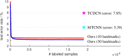
Landmark detection with few labeled samples.
Taking our model as a detector of manually annotated landmarks, we find that less than 200 samples are enough for our model to achieve less than 4% mean error on the MAFL testing set, which is better than the performance of TCDCN and MTCNN. Learning curves are provided in Appendix F.1.
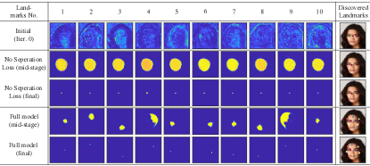
Effectiveness of different loss terms.
Our method combines several loss terms in the training objective (15). Table 1c shows that the removal of any term can cause performance drop of our model. In particular, the removal of the separation loss can devastate the model, and more detailed discussion about this loss term is in Appendix F.2. Our new differentiable formulation of the landmark validity constraints can already lead to a lower landmark detection error than Thewlis et al. [59]’s. Adding the reconstruction loss can further improve the accuracy.
| Dataset | Car | Cat head | Human3.6M | ||
|---|---|---|---|---|---|
| # discovered landmarks | 10 | 24 | 10 | 20 | 16 |
| Thewlis et al. [59] | 11.42 | 11.11 | 26.76 | 26.94 | 7.51 |
| Ours | 05.87 | 05.80 | 15.35 | 14.84 | 4.14 |
4.3 Visual attribute recognition
| Methods |
|
|
|
|
|
|
|
|
|
|
|
|
|
Smiling | Average | |||||||||||||||||||||||||||||
|---|---|---|---|---|---|---|---|---|---|---|---|---|---|---|---|---|---|---|---|---|---|---|---|---|---|---|---|---|---|---|---|---|---|---|---|---|---|---|---|---|---|---|---|---|
| Ours (discovered landmarks) | 60 | 79.4 | 80.9 | 76.9 | 82.3 | 94.5 | 82.5 | 88.4 | 81.3 | 88.0 | 73.2 | 73.7 | 92.1 | 88.8 | 83.2 | |||||||||||||||||||||||||||||
| FaceNet [51] (top-layer) | 128 | 76.4 | 80.3 | 76.8 | 80.4 | 94.5 | 72.6 | 82.7 | 74.4 | 87.9 | 72.7 | 73.1 | 92.2 | 76.2 | 80.0 | |||||||||||||||||||||||||||||
| FaceNet (top-layer) + Ours | 188 | 81.3 | 81.3 | 77.5 | 82.6 | 94.5 | 83.5 | 91.2 | 83.8 | 88.4 | 73.7 | 75.0 | 92.7 | 89.9 | 84.3 | |||||||||||||||||||||||||||||
| FaceNet [51] (conv-layer) | 1792 | 78.8 | 81.5 | 77.4 | 80.5 | 94.6 | 77.3 | 90.0 | 80.9 | 88.4 | 74.2 | 73.6 | 92.4 | 81.5 | 82.4 | |||||||||||||||||||||||||||||
| FaceNet (conv-layer) + Ours | 1852 | 80.1 | 81.8 | 77.2 | 82.3 | 94.7 | 82.1 | 90.8 | 85.0 | 88.6 | 74.5 | 73.6 | 92.4 | 90.5 | 84.1 |
Landmarks reflect object shapes. We use our discovered landmarks as a feature representation to recognize the shape-related binary facial attributes (13 labeled attributes are found) on CelebA. We still take the MAFL testing set for the quantitative evaluation. A linear SVM is trained for each attribute on the CelebA training set. We also compare our landmark coordinates with pretrained FaceNet [51] (InceptionV1) top-layer (128-dim) and top conv-layer (1792-dim) features for the attribute recognition task. As shown in Table 3, our discovered landmarks (60-dim) outperforms the FaceNet top-layer features for most attributes. The conv-layer features outperform our landmarks slightly but have a much higher dimension. Combining the landmark coordinates and the FaceNet features, higher accuracy is achieved. This suggests that the discovered landmarks are complementary to image features pretrained on classification tasks.
4.4 Image manipulation and generation
Our jointly trained image decoding module conditioned its outputs on the input landmarks and their latent descriptors. If the two conditions are disentangled, we should be able to manipulate the object shape without changing other appearance factors by adjusting only the landmarks; or, vice versa. Note that landmark-based image morphing is not a new topic, and landmark-based hierarchical image decoding has also been explored recently [46, 64, 47]. However, these landmarks are all designed and annotated by humans. So far, little evidence has suggested that the automatically discovered landmarks are accurate and representative enough as a reliable condition for image generation.
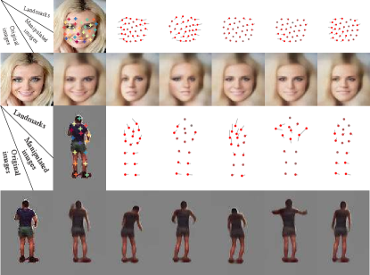
In Figure 10, we synthesize flows to adjust the discovered landmarks of an input image. Fixing the landmark latent descriptors, we obtain realistic facial and human-body images whose shapes agree with the new landmarks. Other than the facial and body shape, then appearance factors of the input image are not visually changed. This result suggests that our image decoding module can synthesize realistic image using the landmarks learned without supervision, and it also suggests that our discovered landmarks have become an explicit representation disentangled from other factors of variations for image modeling. Implementation details and more results about unsupervised landmark-based face manipulation are available in Appendix A.

In Figure 11, instead of adjusting the landmark coordinates, we use the discovered landmarks of a reference image as the control signal to generate new facial images. Following the GAN framework [18], the latent representation of the generated image is randomly drawn from a prior distribution. As in Reed et al. [46], the landmark coordinates and latent representation are combined for image generation. We adopt BEGAN [3] for the discriminator and training objective. In addition, we apply a cyclic loss for the landmark coordinates, which encourages the same landmarks to be detected on the generated images as on the reference image. Our results provide additional evidence on the usefulness of the discovered landmarks for image modeling. Implementation details are in Appendix G.5.
5 Conclusion
We address the problem of unsupervised object landmark discovery and take it as an intermediate step of image representation learning. In particular, a fully differentiable neural network architecture is proposed for determining the landmark coordinates, together with soft contraints to enforce the validity of the detected landmarks. The discovered landmarks are visually meaningful and quantitatively more relevant to human-designed landmarks. In our framework, the discovered landmarks are an explicit part of the learned image representations. They are disentangled from the latent representations of the other appearance factors. The landmark-based explicit representations not only provide an interface for manipulating the image generation process but also appear to be complementary to pretrained deep-neural-network features for solving discriminative tasks.
Acknowledgements
This work was supported in part by ONR N00014-13-1-0762, NSF CAREER IIS-1453651, and Sloan Research Fellowship.
References
- Bau et al. [2017] David Bau, Bolei Zhou, Aditya Khosla, Aude Oliva, and Antonio Torralba. Network dissection: Quantifying interpretability of deep visual representations. In CVPR, 2017.
- Bengio et al. [2007] Yoshua Bengio, Pascal Lamblin, Dan Popovici, and Hugo Larochelle. Greedy layer-wise training of deep networks. In NIPS, 2007.
- Berthelot et al. [2017] David Berthelot, Tom Schumm, and Luke Metz. BEGAN: Boundary equilibrium generative adversarial networks. arXiv preprint arXiv:1703.10717, 2017.
- Bookstein [1989] Fred L. Bookstein. Principal warps: Thin-plate splines and the decomposition of deformations. IEEE Transactions on Pattern Analysis and Machine Intelligence, 11(6):567–585, 1989.
- Burgos-Artizzu et al. [2013] Xavier P Burgos-Artizzu, Pietro Perona, and Piotr Dollár. Robust face landmark estimation under occlusion. In ICCV, 2013.
- Burl et al. [1998] Michael C Burl, Markus Weber, and Pietro Perona. A probabilistic approach to object recognition using local photometry and global geometry. In ECCV, 1998.
- Cao et al. [2014] Xudong Cao, Yichen Wei, Fang Wen, and Jian Sun. Face alignment by explicit shape regression. International Journal of Computer Vision, 107(2):177–190, 2014.
- Catalin Ionescu [2011] Cristian Sminchisescu Catalin Ionescu, Fuxin Li. Latent structured models for human pose estimation. In ICCV, 2011.
- Cho et al. [2015] Minsu Cho, Suha Kwak, Cordelia Schmid, and Jean Ponce. Unsupervised object discovery and localization in the wild: Part-based matching with bottom-up region proposals. In The IEEE Conference on Computer Vision and Pattern Recognition (CVPR), June 2015.
- Cootes et al. [2001] Timothy F. Cootes, Gareth J. Edwards, and Christopher J. Taylor. Active appearance models. IEEE Transactions on Pattern Analysis and Machine Intelligence, 23(6):681–685, 2001.
- Cristinacce and Cootes [2008] David Cristinacce and Tim Cootes. Automatic feature localisation with constrained local models. Pattern Recognition, 41(10):3054–3067, 2008.
- Dantone et al. [2012] Matthias Dantone, Juergen Gall, Gabriele Fanelli, and Luc Van Gool. Real-time facial feature detection using conditional regression forests. In CVPR, 2012.
- Eigen et al. [2014] David Eigen, Christian Puhrsch, and Rob Fergus. Depth map prediction from a single image using a multi-scale deep network. In NIPS, 2014.
- Fan et al. [2017] Haoqiang Fan, Hao Su, and Leonidas Guibas. A point set generation network for 3D object reconstruction from a single image. In CVPR, 2017.
- Felzenszwalb et al. [2010] Pedro Felzenszwalb, Ross Girshick, David McAllester, and Deva Ramanan. Object detection with discriminatively trained part-based models. IEEE Transactions on Pattern Analysis and Machine Intelligence, 2010.
- Fergus et al. [2003] Robert Fergus, Pietro Perona, and Andrew Zisserman. Object class recognition by unsupervised scale-invariant learning. In CVPR, 2003.
- Girshick et al. [2016] Ross Girshick, Jeff Donahue, Trevor Darrell, and Jitendra Malik. Region-based convolutional networks for accurate object detection and segmentation. IEEE Transactions on Pattern Analysis and Machine Intelligence, 38(1):142–158, Jan 2016.
- Goodfellow et al. [2014] Ian Goodfellow, Jean Pouget-Abadie, Mehdi Mirza, Bing Xu, David Warde-Farley, Sherjil Ozair, Aaron Courville, and Yoshua Bengio. Generative adversarial nets. In NIPS, 2014.
- Graves et al. [2009] Alex Graves, Marcus Liwicki, Santiago Fernández, Roman Bertolami, Horst Bunke, and Jürgen Schmidhuber. A novel connectionist system for unconstrained handwriting recognition. IEEE Transactions on Pattern Analysis and Machine Intelligence, 31(5):855–868, 2009.
- He et al. [2016] Kaiming He, Xiangyu Zhang, Shaoqing Ren, and Jian Sun. Deep residual learning for image recognition. In CVPR, 2016.
- He et al. [2017] Kaiming He, Georgia Gkioxari, Piotr Dollár, and Ross Girshick. Mask R-CNN. In ICCV, 2017.
- Ionescu et al. [2014] Catalin Ionescu, Dragos Papava, Vlad Olaru, and Cristian Sminchisescu. Human3.6M: Large scale datasets and predictive methods for 3D human sensing in natural environments. IEEE Transactions on Pattern Analysis and Machine Intelligence, 2014.
- Jaderberg et al. [2015] Max Jaderberg, Karen Simonyan, Andrew Zisserman, et al. Spatial transformer networks. In NIPS, 2015.
- Kanazawa et al. [2016] Angjoo Kanazawa, David W Jacobs, and Manmohan Chandraker. WarpNet: Weakly supervised matching for single-view reconstruction. In CVPR, 2016.
- Kingma and Welling [2014] Diederik P Kingma and Max Welling. Auto-encoding variational bayes. ICLR, 2014.
- Krizhevsky et al. [2012] Alex Krizhevsky, Ilya Sutskever, and Geoffrey Hinton. ImageNet classification with deep convolutional neural networks. In NIPS, 2012.
- Lam et al. [2017] Michael Lam, Behrooz Mahasseni, and Sinisa Todorovic. Fine-grained recognition as hsnet search for informative image parts. In CVPR, 2017.
- Lampert et al. [2009] Christoph H Lampert, Hannes Nickisch, and Stefan Harmeling. Learning to detect unseen object classes by between-class attribute transfer. In CVPR, 2009.
- LeCun [1998] Yann LeCun. The MNIST database of handwritten digits. http://yann.lecun.com/exdb/mnist/, 1998.
- Lenc and Vedaldi [2016] Karel Lenc and Andrea Vedaldi. Learning covariant feature detectors. In ECCV Workshop on Geometry Meets Deep Learning, 2016.
- Liu et al. [2015] Ziwei Liu, Ping Luo, Xiaogang Wang, and Xiaoou Tang. Deep learning face attributes in the wild. In ICCV, 2015.
- Long et al. [2015] Jonathan Long, Evan Shelhamer, and Trevor Darrell. Fully convolutional networks for semantic segmentation. In CVPR, 2015.
- Lv et al. [2017] Jiangjing Lv, Xiaohu Shao, Junliang Xing, Cheng Cheng, and Xi Zhou. A deep regression architecture with two-stage re-initialization for high performance facial landmark detection. In CVPR, 2017.
- Maas et al. [2013] Andrew Maas, Awni Hannun, and Andrew Ng. Rectifier nonlinearities improve neural network acoustic models. In ICML, 2013.
- Martin Koestinger and Bischof [2011] Peter Roth Martin Koestinger, Paul Wohlhart and Horst Bischof. Annotated facial landmarks in the wild: A large-scale, real-world database for facial landmark localization. In First IEEE International Workshop on Benchmarking Facial Image Analysis Technologies, 2011.
- Masci et al. [2011] Jonathan Masci, Ueli Meier, Dan Cireşan, and Jürgen Schmidhuber. Stacked convolutional auto-encoders for hierarchical feature extraction. In International Conference on Artificial Neural Networks, 2011.
- Mathieu et al. [2016] Michael F Mathieu, Junbo Jake Zhao, Junbo Zhao, Aditya Ramesh, Pablo Sprechmann, and Yann LeCun. Disentangling factors of variation in deep representation using adversarial training. In NIPS, 2016.
- Matthews and Baker [2004] Iain Matthews and Simon Baker. Active appearance models revisited. International Journal of Computer Vision, 60(2):135–164, 2004.
- Newell et al. [2016] Alejandro Newell, Kaiyu Yang, and Jia Deng. Stacked hourglass networks for human pose estimation. In ECCV, 2016.
- Noh et al. [2015] Hyeonwoo Noh, Seunghoon Hong, and Bohyung Han. Learning deconvolution network for semantic segmentation. In ICCV, 2015.
- Novotny et al. [2017] David Novotny, Diane Larlus, and Andrea Vedaldi. AnchorNet: A weakly supervised network to learn geometry-sensitive features for semantic matching. 2017.
- Pedersoli et al. [2014] Marco Pedersoli, Tinne Tuytelaars, and Luc Van Gool. Using a deformation field model for localizing faces and facial points under weak supervision. In CVPR, 2014.
- Radford et al. [2016] Alec Radford, Luke Metz, and Soumith Chintala. Unsupervised representation learning with deep convolutional generative adversarial networks. In ICLR, 2016.
- Reed et al. [2014] Scott Reed, Kihyuk Sohn, Yuting Zhang, and Honglak Lee. Learning to disentangle factors of variation with manifold interaction. In ICML, 2014.
- Reed et al. [2015] Scott Reed, Yi Zhang, Yuting Zhang, and Honglak Lee. Deep visual analogy-making. In NIPS, December 2015.
- Reed et al. [2016] Scott Reed, Zeynep Akata, Santosh Mohan, Samuel Tenka, Bernt Schiele, and Honglak Lee. Learning what and where to draw. In NIPS, 2016.
- Reed et al. [2017] Scott Reed, Aäron van den Oord, Nal Kalchbrenner, Sergio Gómez Colmenarejo, Ziyu Wang, Dan Belov, and Nando de Freitas. Parallel multiscale autoregressive density estimation. In ICML, 2017.
- Ren et al. [2014] Shaoqing Ren, Xudong Cao, Yichen Wei, and Jian Sun. Face alignment at 3000 FPS via regressing local binary features. In CVPR, 2014.
- Ren et al. [2015] Shaoqing Ren, Kaiming He, Ross Girshick, and Jian Sun. Faster R-CNN: Towards real-time object detection with region proposal networks. In NIPS, 2015.
- Rocco et al. [2017] Ignacio Rocco, Relja Arandjelović, and Josef Sivic. Convolutional neural network architecture for geometric matching. In CVPR, 2017.
- Schroff et al. [2015] Florian Schroff, Dmitry Kalenichenko, and James Philbin. FaceNet: A unified embedding for face recognition and clustering. In CVPR, 2015.
- Sicre et al. [2017] Ronan Sicre, Yannis Avrithis, Ewa Kijak, and Frédéric Jurie. Unsupervised part learning for visual recognition. In CVPR, 2017.
- Simonyan and Zisserman [2015] Karen Simonyan and Andrew Zisserman. Very deep convolutional networks for large-scale image recognition. In ICLR, 2015.
- Singh et al. [2012] Saurabh Singh, Abhinav Gupta, and Alexei A Efros. Unsupervised discovery of mid-level discriminative patches. In ECCV, 2012.
- Sun et al. [2013] Yi Sun, Xiaogang Wang, and Xiaoou Tang. Deep convolutional network cascade for facial point detection. In CVPR, 2013.
- Szegedy et al. [2015] Christian Szegedy, Wei Liu, Yangqing Jia, Pierre Sermanet, Scott Reed, Dragomir Anguelov, Dumitru Erhan, Vincent Vanhoucke, Andrew Rabinovich, et al. Going deeper with convolutions. In CVPR, 2015.
- Tang et al. [2014] Kevin Tang, Armand Joulin, Li-Jia Li, and Li Fei-Fei. Co-localization in real-world images. In CVPR, 2014.
- Thewlis et al. [2017a] James Thewlis, Hakan Bilen, and Andrea Vedaldi. Unsupervised learning of object frames by dense equivariant image labelling. In NIPS, 2017a.
- Thewlis et al. [2017b] James Thewlis, Hakan Bilen, and Andrea Vedaldi. Unsupervised learning of object landmarks by factorized spatial embeddings. In ICCV, 2017b.
- Toshev and Szegedy [2014] Alexander Toshev and Christian Szegedy. DeepPose: Human pose estimation via deep neural networks. In CVPR, 2014.
- Valstar et al. [2010] Michel Valstar, Brais Martinez, Xavier Binefa, and Maja Pantic. Facial point detection using boosted regression and graph models. In CVPR, 2010.
- van den Oord et al. [2016] Aaron van den Oord, Nal Kalchbrenner, Lasse Espeholt, Oriol Vinyals, Alex Graves, et al. Conditional image generation with pixelcnn decoders. In NIPS, 2016.
- Van Oord et al. [2016] Aaron Van Oord, Nal Kalchbrenner, and Koray Kavukcuoglu. Pixel recurrent neural networks. In ICML, 2016.
- Villegas et al. [2017] Ruben Villegas, Jimei Yang, Yuliang Zou, Sungryull Sohn, Xunyu Lin, and Honglak Lee. Learning to generate long-term future via hierarchical prediction. In ICML, 2017.
- Wang and Gupta [2016] Xiaolong Wang and Abhinav Gupta. Generative image modeling using style and structure adversarial networks. In ECCV, 2016.
- Weber et al. [2000] Markus Weber, Max Welling, and Pietro Perona. Towards automatic discovery of object categories. In CVPR, 2000.
- Wu et al. [2016] Jiajun Wu, Tianfan Xue, Joseph J Lim, Yuandong Tian, Joshua B Tenenbaum, Antonio Torralba, and William T Freeman. Single image 3D interpreter network. In ECCV, 2016.
- Wu et al. [2017] Yue Wu, Chao Gou, and Qiang Ji. Simultaneous facial landmark detection, pose and deformation estimation under facial occlusion. In CVPR, 2017.
- Xiang et al. [2014] Yu Xiang, Roozbeh Mottaghi, and Silvio Savarese. Beyond PASCAL: A benchmark for 3D object detection in the wild. In WACV, 2014.
- Xiao et al. [2016] Shengtao Xiao, Jiashi Feng, Junliang Xing, Hanjiang Lai, Shuicheng Yan, and Ashraf Kassim. Robust facial landmark detection via recurrent attentive-refinement networks. In ECCV, 2016.
- Xiao et al. [2017] Shengtao Xiao, Jiashi Feng, Luoqi Liu, Xuecheng Nie, Wei Wang, Shuicheng Yan, and Ashraf Kassim. Recurrent 3d-2d dual learning for large-pose facial landmark detection. In ICCV, 2017.
- Yang et al. [2016] Wei Yang, Wanli Ouyang, Hongsheng Li, and Xiaogang Wang. End-to-end learning of deformable mixture of parts and deep convolutional neural networks for human pose estimation. In CVPR, pages 3073–3082, 2016.
- Yang [2013] Yi Yang. Articulated Human Pose Estimation with Flexible Mixtures of Parts. PhD thesis, University of California, Irvine, 2013.
- Yu and Grauman [2014] Aron Yu and Kristen Grauman. Fine-grained visual comparisons with local learning. In CVPR, 2014.
- Yu et al. [2016] Xiang Yu, Feng Zhou, and Manmohan Chandraker. Deep deformation network for object landmark localization. In ECCV, 2016.
- Zeiler and Fergus [2014] Matthew D. Zeiler and Rob Fergus. Visualizing and understanding convolutional networks. In ECCV, 2014.
- Zhang et al. [2014a] Jie Zhang, Shiguang Shan, Meina Kan, and Xilin Chen. Coarse-to-fine auto-encoder networks (CFAN) for real-time face alignment. In ECCV, 2014a.
- Zhang et al. [2016a] Kaipeng Zhang, Zhanpeng Zhang, Zhifeng Li, and Yu Qiao. Joint face detection and alignment using multitask cascaded convolutional networks. IEEE Signal Processing Letters, 2016a.
- Zhang et al. [2008] Weiwei Zhang, Jian Sun, and Xiaoou Tang. Cat head detection - how to effectively exploit shape and texture features. ECCV, 2008.
- Zhang et al. [2015] Yuting Zhang, Kihyuk Sohn, Ruben Villegas, Gang Pan, and Honglak Lee. Improving object detection with deep convolutional networks via Bayesian optimization and structured prediction. In CVPR, 2015.
- Zhang et al. [2014b] Zhanpeng Zhang, Ping Luo, Chen Change Loy, and Xiaoou Tang. Facial landmark detection by deep multi-task learning. In ECCV, 2014b.
- Zhang et al. [2016b] Zhanpeng Zhang, Ping Luo, Chen Change Loy, and Xiaoou Tang. Learning deep representation for face alignment with auxiliary attributes. IEEE Transactions on Pattern Analysis and Machine Intelligence, 38(5):918–930, 2016b.
- Zhu and Ramanan [2012] Xiangxin Zhu and Deva Ramanan. Face detection, pose estimation, and landmark localization in the wild. In CVPR, 2012.
Appendices
Unsupervised Discovery of Object Landmarks as Structural Representations
Yuting Zhang1, Yijie Guo1, Yixin Jin1, Yijun Luo1, Zhiyuan He1, Honglak Lee2,1
1University of Michigan, Ann Arbor 2Google Brain
{yutingzh, guoyijie, jinyixin, lyjtour, zhiyuan, honglak}@umich.edu honglak@google.com
.tocmtappendix \etocsettagdepthmtchapternone \etocsettagdepthmtappendixsubsection
The project web page (code and results): http://ytzhang.net/projects/lmdis-rep
Supplementary videos referred to in the appendices can be obtained at http://ytzhang.net/files/lmdis-rep/supp-videos.tar.gz
Appendix A More details and results on face manipulation using unsupervised landmarks
The discovered landmarks constitute the explicitly structural part of the image representation learned by our model. They provide an interface for humans to manipulate the image representation intuitively. Our decoding module can generate realistic facial images using the landmark descriptors extracted from a given image and different sets of landmarks.
In addition to the results shown in the main paper, we provide more qualitative results for unsupervised landmark-based face manipulation in this section. We train models of 10, 20, and 30 landmarks. To evaluate our method on many target landmarks, we take the landmarks discovered from other images and the interpolation/extrapolation between the landmarks discovered on two images as the targets.
In this section, we show results for our 30-landmark model (results for our 10,20-landmark model are available as supplementary videos). Figure 12 and 13 show results for manipulating all 30 landmarks. Figure 14 and 15 show results for manipulating the 3 landmarks at the mouth. Figure 16 and 17 show results for manipulating the 5 landmarks at the mouth and jaw. Videos are available in the following folders for gradually morphing the landmarks from their original coordinates to the target by linear interpolation.
-
•
30-landmark models: videos/face.30landmark-model.manipulate-{all|mouth|mouthext}-landmarks
-
•
10,20-landmark models: videos/face.{10|20}landmark-model.manipulate-{all|mouth}-landmarks
See next page for the figure.


Appendix B Our model without landmark descriptors on MNIST
We train our landmark discovery model without the landmark descriptor pathway on MNIST in two settings: one model for each digit (Appendix B.1) and one model for all ten digits (Appendix B.2). Using the model for all digits, we can perform geometrically meaningful morphing between different digits (Appendix B.3), e.g., morphing 2 to 9. Videos for the morphing process are available in the folder videos/mnist-morphing .
B.1 Models for individual digits
In this section, our landmark discovery model is trained for each digit independently. As shown in Figure 18, the discovered landmarks are consistent within each digit despite the shape variations.
B.2 Models for all digits
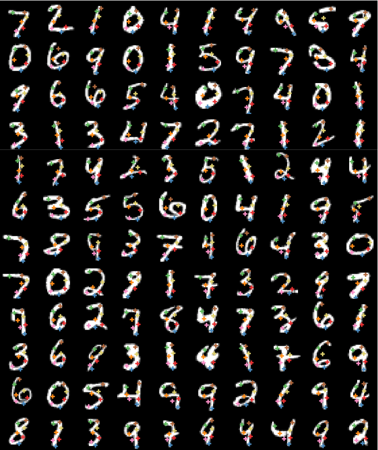
In this section, we train a single model for all ten digits together. In Figure 19, the corresponding landmarks are shown in the same color. The landmarks discovered on the same digits are consistent across different image. More interesting, the corresponding landmarks across different digits are also semantically consistent. For examples, the orange cross is always in the middle of a digits, the blue cross at the bottom, and the green one at the most left-top part of every digit.
B.3 Digit morphing using discovered landmarks
Our model trained on the mix of all ten digits can discover corresponding patterns among different digit categories. Using this model, we can perform geometrically meaningful cross-category morphing. Figure 20 and 21 illustrate the morphing process. Note that the landmark coordinates constitute the full image representation for MNIST digits. Videos for the morphing process are available in the folder videos/mnist-morphing .


Appendix C Details and more results on Human3.6M
On the Human3.6M dataset, we train our landmark discovery model on six actions: waiting, posing, greeting, directions, discussions, and walking. We report quantitative results on predicting the 32 annotated landmarks555Some markers are close to each other (e.g., on each foot, there are two markers), so the effective locations annotated by the markers are less than 32 (around 16). (acquired by wearable markers) using our models trained for the mix of all six actions and each independent action. We also show qualitative results of the mixed-action model (trained for all six actions).
C.1 Optical flow as self-supervision for equivariance
The Human3.6M training data is in the video format. We can calculate the optical flows between nearby frames and take them as self-supervision for the equivariance constraint defined in (8). Following the same notations, the two frames are and , and the optical flows define the transformation . In particular, we use the Farneback method in OpenCV to compute the dense optical flows at 5-frame intervals. We then accumulate two optical flow fields to calculate the optical flows at 10-frame intervals. The 10-frame-interval optical flow fields in addition to the random TPS transform are used in the equivariance constraint.
Note that using optical flow as the self-supervision for the equivariance constraint can push the landmarks to the background region. This phenomenon occurs because locating landmarks at image regions with weaker optical flows can result in low equivariance loss. To prevent trivial landmarks, we encourage the landmarks to be discovered at locations with strong optical flows. Let and be the components of the optical flow map from the current image to another frame. The flow magnitude map is . Recall that is the multi-channel heatmap computed from the landmark locations. We encourage and to have a significant correlation. In particular, loss to encourage
| (16) |
We use the same loss weight for as .
Using the above formulation, we can reduce the ground landmark prediction error from (without optical flows) to (with optical flows). For all experiments on Human3.6M, we use the optical flow as self-supervision for equivariance as described above.
C.2 Quantitative results
We compare our model with Thewlis et al. [59]’s unsupervised landmark discovery method regarding the annotated-landmark prediction accuracy. Both models discover 16 landmarks. The whole training set is used to train the linear mapping from the discovered landmarks to the annotated ones. As discussed in the main paper, we do not expect the two unsupervised methods to distinguish the frontal and back views. Thus, in the evaluation, we compute the errors against the original landmark annotations and its left-right-flipped counterpart666For examples, we swap the coordinates of the left-shoulder landmark and the right-shoulder landmark. , and then we choose the minimum value as the final error. Note that, when flipping the landmark annotations, the landmarks for the whole body are flipped simultaneously. As to the linear regressor training, we propose the following training strategy.
-
1.
Figure out the rough orientations of the human body, heuristically. If more than 2/3 of the left-hand side annotated landmarks are to the right of the right-hand side annotated landmarks, the human is in the frontal view.
-
2.
Train the regressor using the images with the landmark annotations in the frontal view. The other images are ignored in this step.
-
3.
Use the aforementioned evaluation protocol to determine if the landmark annotations on other images should be flipped or not. The model is then retrained with all the training images.
-
4.
Repeat the step 3 until the model is converged.
As shown in Table 4, our method outperforms Thewlis et al. [59]’s method significantly. We also report the results obtained by Newell et al. [39]’s supervised stacked hourglass network using their off-the-shelf pretrained 16-landmark model. Both unsupervised methods perform worse than the supervised stacked hourglass network. However, our model is unsupervised, and our neural network architectures are also smaller. We believe that our results show the potential of unsupervised methods for discovering complicated object structures.
| Methods |
|
Waiting | Posing | Greeting | Directions | Discussion | Walking | |||
|---|---|---|---|---|---|---|---|---|---|---|
| Unsupervised | Thewlis et al. [59] | 7.51 | 7.54 | 8.56 | 7.26 | 6.47 | 7.93 | 5.40 | ||
| Ours (discovered landmarks) | 4.14 | 5.01 | 4.61 | 4.76 | 4.45 | 4.91 | 4.61 | |||
| Supervised | Hourglass Newell et al. [39] | 2.16 | 1.88 | 1.92 | 2.15 | 1.62 | 1.88 | 2.21 | ||
C.3 Qualitative results
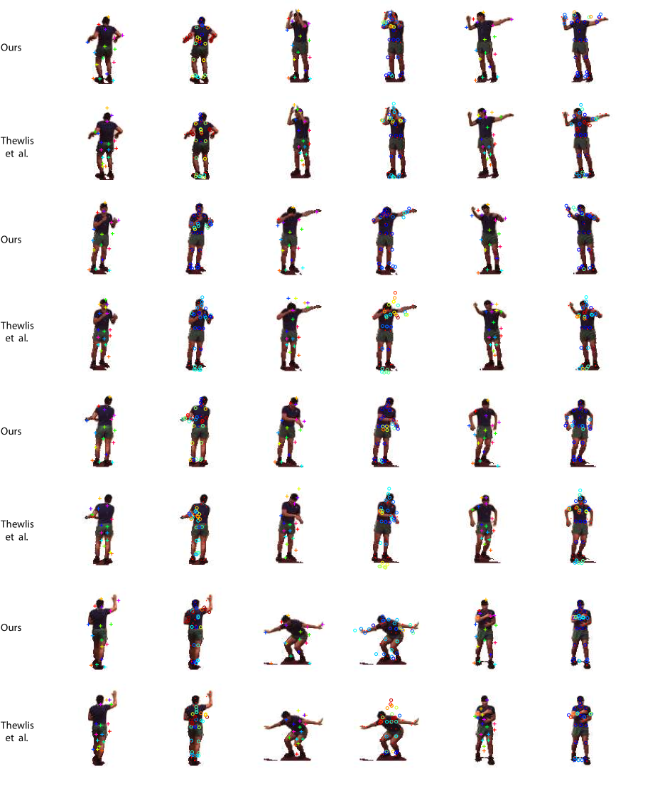
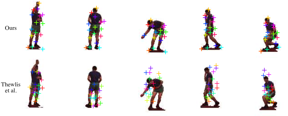
We train our model and Thewlis et al. [59]’s model on all six chosen actions and perform the annotated-landmark prediction. Figure 22 shows the side-by-side comparison. In general, our method visually outperforms Thewlis et al. [59]’s. Figure 23 shows landmark discovery examples, where our method outperforms Thewlis et al. [59]’s method very significantly.
See next page for the figure.
 |

Appendix D Results on animals of mixed species
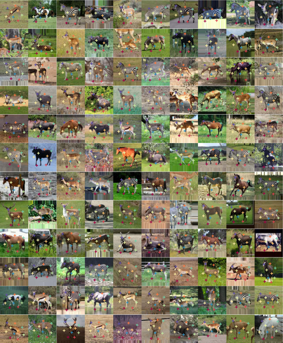
On the animal-with-attributes (AwA) dataset [28], we choose the profile images from five animal categories (antelope, deer, moose, horse, zebra) and try to detect landmarks on these mixed species of animals. As shown in Figure 24, even though multiple species of animals with different appearance are mixed, our method can still find several consistent landmarks. For example, the yellow cross is always on the hoof, the orange cross always above the back and the light green cross at the buttock. The landmarks are consistently detected despite the significant variations in species, pose and individual appearance.
See next page for the figure.
Appendix E More qualitative results on human faces, cat heads, cars, and shoes
In this section, we show more result of landmark discovery and ground truth landmark prediction compared with Thewlis et al. [59]. All the shown images are randomly sampled from the test set.
E.1 CelebA
 |
E.2 AFLW
E.3 Cat heads
 |
E.4 Cars
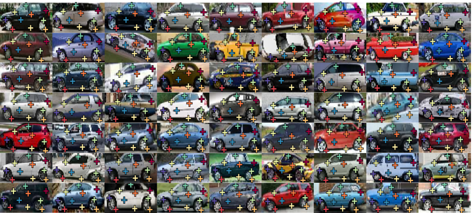
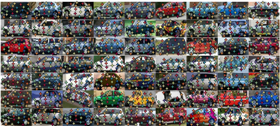
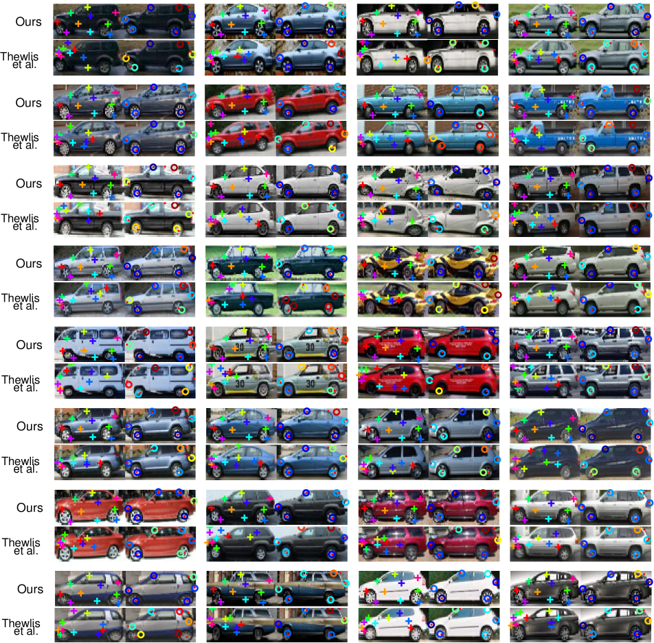 |
E.5 Shoes
Appendix F Ablative study
F.1 Number of labeled samples for annotated-landmark prediction
Taking our model as a detector of manually annotated landmarks, we find that less than 200 samples are enough for our model to achieve less than 4% mean error on the MAFL testing set, which is better than the performance of two popular off-the-shelf models. This result suggests that it is possible to train a high-accurate landmark detector using only a few labeled sample when sufficient unlabeled samples are given to train our unsupervised model. We show its performance versus the number of labeled samples in Figure 38.
F.2 Evolution of detection confidence map during training
Figure 39 shows the detection confidence maps of an input image at different training stage of our model. In the beginning, the heatmap shows random values over the whole image. As a result, the landmarks, defined as the mean coordinates weighted by the confidence maps, are all at the center of the image. As the training goes on, the values gradually becomes spatially concentrated. With the separation loss defined in (7), the peaked value of each channel of the confidence map can move to a different location. Without the separation loss, every channel can have a peaked value at the center of the images, resulting in degenerate landmarks.
F.3 TPS control points
For the random TPS in our equivariance constraint (defined in (8)), we both use the regular-grid control points and take the discovered landmarks in the current iteration as the control points. The two sets of control points are alternatively used in each optimization iteration with 73 chance. We do not exhaustively tune the ratio and keep it the same in all experiments. As shown in Figure 5, the performance of our model is fairly insensitive to this ratio when the other hyper-parameters are fixed. However, introducing the discovered landmarks as the TPS control points does benefit.
| gridlandmark | 10:0 | 1:9 | 3:7 | 5:5 | 7:3 | 9:1 |
| GT prediction error / % | 4.17 | 3.86 | 3.46 | 3.38 | 3.46 | 3.41 |
Note that the discovered landmarks are clustered at the center of the image (see discussion about the separation constraint in Section 3.2) and cannot serve as good TPS control points. As a result, we use only the regular-grid control points in the beginning and start to apply the previously mentioned ratio after training the model for several thousands of iterations.
Appendix G Implementation details
G.1 Data preprocessing
The main paper and this supplementary materials report results on several datasets. Table 6 summarizes the image size we used for each each dataset. In our landmark discovery formulation, we need to perform random TPS to calculate the equivariance constraint in (8). It requires the image to have large enough margins so that the foreground will not be out of image due to the random transformation. Table 6 also summarizes the image size after padding with the edge values.
| Dataset | Image size | Padded size | Remark |
|---|---|---|---|
| CelebA, AFLW, Cat Heads, Shoes | 8080 | 9696 | - |
| Profile Cars from PASCAL 3D | 6464 | 9696 | visualized as |
| Animals from AwA | 6464 | 8080 | - |
| Human3.6M | 128128 | 192192 | - |
| MNIST | 2828 | 5656 | - |
For different datasets, we crop the foreground images and prepare input images as follows.
- CelebA
-
We started from the cropped-and-aligned images (218178) in CelebA dataset, scaled them to 100100 pixels and then cropped the 8080 center patches.
- AFLW
-
The dataset provides annotated bounding boxes. We enlarged the bounding boxes on each image with a margin on the top ( height of the original bounding box), margins on the left and right ( width of the original bounding box) so that the cropped facial images look similar to the CelebA data. The cropped images were also scaled to 8080.
- Cat Heads
-
The dataset provides ground truth landmarks on the cat head. We figured out the bounding box for cropping each image according to the landmarks and then scaled the cropped images to 8080.
- Shoes
-
We scaled the shoe images (102136) to 6464, and padded the images to be 8080 with white margins. We linearly transformed the color value range from to to avoid a huge amount of saturated responses for the output layer with the sigmoid activation. The color was scaled back for visualization.
- Cars
-
The PASCAL 3D dataset provides annotations for the orientation and landmarks of several objects. We cropped the profile car images according to the bounding box of the ground truth landmarks. Slight margins are added to the bounding box, and the cropped image is scaled to a square image without preserving the aspect ratio.
- Animals from AwA
-
We manually annotated bounding boxes and orientation labels (i.e., left, right, frontal, back) for several types of animals. For each rectangular bounding box, we enlarged its shorter edge to make the box square, cropped the patch, and scaled it to 6464. We ignored the images with frontal and back views, and we flipped the right-facing animals horizontally so that all animals in the image face to the left.
- Human3.6M
-
The human body was cropped using a square bounding box from the original video frames. We use the 3D landmarks provided in this dataset, acquired by wearable markers, as side information to roughly align the scales and foot locations of the human bodies in different images. The cropped square images are scaled to 128128 pixels. We use the provided segmentation masks, obtained by an off-the-shelf unsupervised background removal method, to mask out the background image with gray color. For visualization, we show the gray color as white for the printing clarity.
? *: decided by the number of landmarks. ? **: decided by the number of landmarks and the dimension of the shared feature space. ? ***: this layer is used only for , and the number of channels is decided by the number of landmarks. ? ****: decided by the number of landmarks for , for , and for . Each skip-link in (a), (b), (c), (d), and (f) consists of three convolutional layers of 33 kernels. Each skip-link in (e), (g), and (h) consists of two convolutional layers of 33 kernels.
G.2 Network architectures
In Section 3 of the main paper, we describe the key architectures of our model and leave some details unspecified. This section describes the detailed neural network architectures.
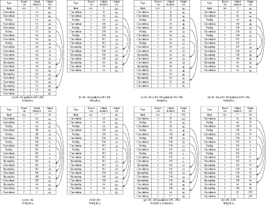
Figure 40 summarizes the hourglass-like architectures that we used for images of different sizes. The image padding is explaned and specified in Appendix G.1. In general, an hourglass architecture has mirrored encoding (high-resolution to low-resolution) and decoding (low-resolution and high-resolution) architectures. Skip-links, made up of convolutional layers, create shortcuts from the encoding feature maps and decoding feature maps of the same resolution. The responses of the skip-links are fused with the main stream decoding responses using element-wise addition. We use the max-pooling to reduce the feature map size for encoding, and we upsample feature maps by the nearest interpolation for decoding. For each linear layer, a batch normalization layer is followed, and LeakyReLU [34] is the default activation function.
Based on the neural network architectures in Figure 40, a convolutional layer of 11 kernels calculates the raw detection score map of channels (recall that is the number of landmarks). For image output, the last convolutional layer’s responses () are mapped to with a sigmoid function for the reconstructed color intensity and to by for the pixel-wise standard deviation, respectively.
G.3 Training strategy
We use Adam with an initial learning rate of to optimize the neural network parameters. We set the training batch size to 16 or 32777There is no significant difference in the performance when using either 16 or 32 as the training batch size. for 8080 and 6060 images and 8 for 128128 images. The learning rate starts from and decreases to and later. For color images, we do random brightness and contrast jittering.
For batch normalization, the global mean and variance are computed using a random subset of the training set when the neural network training is done. Note that using the running average during training for the global mean and variance can hurt the performance.
To implement the equivariance constraint in (8), we use random TPS transformation to obtain warped input images (paired with the original images) in each training iteration. Taking the normalized image height and width as , the random transformation parameters are:
-
•
Global affine component. Uniform random translation in ; Gaussian random rotation with the standard deviation of ; Gaussian random scaling in the base- logarithm scale with the standard deviation of .
-
•
Local TPS. Gaussian random translation with the standard deviation of (regarding the regular-grid control points) or (regarding the landmark control points).
For the reconstruction loss weight in (15), we find it helpful to start with a small value and increase it to its final value at a later stage. At the early training stage, the discovered landmarks change significantly for each iteration, and the latent descriptor of landmarks inputted to the decoder also varies a lot. The model parameters of the decoder and the gradients from it can change too drastically if the reconstruction loss weights is large, which would harm the training of both the landmark detector and the landmark-based image decoder. As a particular training strategy, we increase the value of by twice during the training. Table 7 in Appendix G.4 summarizes the detailed hyper-parameters.
For the L2 reconstruction loss , we scale the image pixel values to . The loss is explicitly defined as the negative logarithm likelihood (NLL) to draw the input image from the Gaussian distribution centered at the reconstructed image the with a fix variation . More specifically,
| (17) |
The value of the loss weight is based on this definition.
G.4 Hyper-parameters
Table 7 summarizes the dataset-specific hyper-parameters. Note that our model is not sensitive to minor changes of the hyper-parameters, but adjusting the hyper-parameters for each dataset can improve the performance slightly.
| Dataset | # landmark | 1st LR decay iter. | 2nd LR decay iter. | Initial | 1st increase iter. | 2nd increase iter. | |||||
| CelebA | 10 | 100K | 200K | 0.01 | 100K | 200K | 100 | 0.06 | 16 | 8 | |
| CelebA | 30 | 100K | 200K | 0.1 | 100K | 200K | 100 | 0.04 | 10 | 8 | |
| AFLW | 10 | 100K | 200K | 0.1 | 100K | 200K | 100 | 0.06 | 16 | 8 | |
| AFLW | 30 | 100K | 200K | 0.0001 | 100K | 200K | 100 | 0.04 | 10 | 8 | |
| Cat | 10 | 100K | 200K | 0.0001 | 100K | 200K | 100 | 0.08 | 20 | 8 | |
| Cat | 20 | 100K | 200K | 0.0001 | 100K | 200K | 100 | 0.05 | 10 | 8 | |
| Car | 10 | 40K | 80K | 0.001 | 40K | 50K | 100 | 0.08 | 200 | 8 | |
| Car | 24 | 40K | 80K | 0.001 | 40K | 50K | 100 | 0.05 | 200 | 8 | |
| Animal | 10 | 20K | 50K | 0.001 | 40K | 50K | 100 | 0.08 | 20 | 2 | |
| Shoes | 8 | 100K | 20K | 0.01 | 100K | 200K | 100 | 0.05 | 20 | 8 | |
| Human | 16 | 100K | 200K | 0.1 | 100K | 200K | 100 | 0.06 | 20 | 8 |
G.5 Details about face generations using unsupervised landmarks
Figure 11 in the main paper shows results of generating facial images conditioned on our discovered landmarks. In this experiment, we fix our landmark discovery module and use it to detect landmarks on training images. For the decoding module, we take the detected landmarks as a given input condition and map an isotropic Gaussian random variable to the latent part of the image representation. Inspired by [46], we first use deconvolutional layers to get a feature map from the random variable and use convolutional layers to get another map of the same size from the reconstructed detection confidence map. We use element-wise multiplication and channel-wise concatenation to fuse the two into one feature map as the input of the decoding neural network. Thus, the way of calculating the input feature map of the decoding module is not the same as our landmark discovery model.
We use the boundary equilibrium GAN (BEGAN) [3] framework to design the discriminator, which encourages the decoder to generate realistic images. More concretely, an autoencoder is trained as the energy function to distinguish the real and generated images. To make sure the generated images are consistent with the landmark condition, we first use our landmark discovery module to detect landmarks on them. We then take the L1 distance between them and those from the corresponding real images (i.e., input training images for getting the landmarks) as an extra training loss for the decoding module.
This experiment is mainly to show that our discovered landmark is accurate and meaningful enough for controllable image generation.