Modified gravity for surveys

Abstract

We present a new parameterization for the equation of state (EoS) $\omega_{X}=P_{X}/\rho_{X}$, which can reproduce a $f(R)$-like evolution with a precision between $[0.5\%-0.8\%]$ over the numerical solutions. Also, our proposal can render a variety of popular $f(R)$ models that are considered as viable candidates for the cosmic late time acceleration. By using observational data from baryonic acoustic oscillations, supernovae and cosmic chronometers we investigate the constraints on the new EoS parameters. This proposal set a EoS formulation which can be used in an efficient way and makes a good candidate to be implemented in a variety of surveys in order to test the $f(R)$ generic behaviour.

I Introduction

Currently, the Universe go through an accelerated expansion, different observations have proved such fact: Supernovae Type Ia (SNIa) Riess:1998cb-Perlmutter:1998np , Baryon Acoustic Oscillations (BAO) Eisenstein:2005su , Cosmic Microwave Background Radiation (CMBR) anisotropies Spergel:2003cb , Large Scale Structure formation Tegmark:2003ud and Weak Lensing Jain:2003tba . Even more, future projects and surveys surveys are underway or being proposed to discover the underlying cause of this phenomena.

The current standard cosmological paradigm is the $\Lambda$CDM model, where $\Lambda$ is a constant term added to the Einstein-Hilbert action. Such addition is performed in order to produce late time acceleration and even when there is no physical ground to justify $\Lambda$, making this model able to fit all the current observations. However, some degrees of tension have appeared among different data sets which has renewed the interest on alternative models that can provide an acceleration mechanism. For instance, the value for the matter density fraction consistent with the Lyman-$\alpha$ forest measurement of the baryon acoustic oscillations Delubac:2014aqe is smaller than the one preferred by CMB measurements. Also, the value of $H_{0}$ inferred from the Planck CMB data Ade:2015xua is $3.4$ $\sigma$ lower than the local measurement reported by Riess:2016jrr . A promising new and independent measurement of $H_{0}$ will come from standard-siren measurements from gravitational waves sources and provide more information on the issue, although the tension linger with the current measurement Abbott:2017xzu .

Using all current observational data, in Zhao:2017cud was reconstructed the Dark Energy equation of state (EoS) obtaining a distinctive shape that crosses multiple times the phantom divide line. This kind of oscillating $\omega_{X}$ can not be produced with a single phantom or quintessence field Shafieloo:2012rs but it can be produced by modified gravity.

Hereafter, we will focus our attention in $f(R)$ gravity models. Their characteristic EoS Jaime:2013zwa makes them an appealing framework in order to reproduce the dynamical evolution of $\omega_{X}$ found in Zhao:2017cud . In regards to the tension issue, in modified gravity theories (e.g. Galileon) may reconcile the Planck with high $H_{0}$ values Barreira:2014jha ; Escamilla-Rivera:2015ova , although known models have problems with either cosmology Renk:2017rzu or gravitational waves Ezquiaga:2017ekz . In this context, the resulting field equations are of fourth order on the metric and behave like attractors; therefore their implementation in the pipeline of surveys, or in N-body, and Boltzmann codes requires many assumptions.

In this paper we present the construction of a new parameterization for the EoS in order to reproduce a variety of $f(R)$ models between $[0.5\%-0.8\%]$ of precision which can help to test these models in a straightforward way. This parameterization can be used as a fiducial model in surveys with the advantage that this one has a physical motivation in comparison to some others like CPL Chevallier:Polarski ; Linder . Future surveys like Euclid 2011arXiv1110.3193L and DESI Levi:2013gra ; Aghamousa:2016zmz will play a fundamental role in the understanding cosmic acceleration and will allow us to test interesting models of gravity and dark energy.

II $f(R)$ cosmology, equation of state and models.

These theories of gravity take a general function of the Ricci scalar in the Einstein-Hilbert action

$$S[g_{ab},{\mbox{\boldmath{$\psi$}}}]=\!\!\int\!\!\frac{f(R)}{2\kappa}\sqrt{-g}\>d^{4}x+S_{\rm matt}[g_{ab},{\mbox{\boldmath{$\psi$}}}]\;,$$ (1)

where $G=c=1$ and $\kappa\equiv 8\pi$, $S_{\rm matt}[g_{ab},{\mbox{\boldmath{$\psi$}}}]$ is the usual action for matter. $f(R)$ is an arbitrary smooth function of the Ricci scalar $R$. The field equations, associated to this action, are given by:

$$f_{R}R_{ab}-\frac{1}{2}fg_{ab}-\left(\nabla_{a}\nabla_{b}-g_{ab}\Box\right)f_{R}=\kappa T_{ab}\,\,,$$ (2)

where $f_{R}=\partial_{R}f$, $\Box=g^{ab}\nabla_{a}\nabla_{b}$ and $T_{ab}$ is the energy-momentum tensor for matter. They can be rewritten as:

$$G_{ab}= \frac{1}{f_{R}}\Bigl{[}f_{RR}\nabla_{a}\nabla_{b}R+f_{RRR}(\nabla_{a}R)(\nabla_{b}R)$$ (3)

$$-\frac{g_{ab}}{6}\Big{(}Rf_{R}+f+2\kappa T\Big{)}+\kappa T_{ab}\Bigl{]},\;$$

where $G_{ab}=R_{ab}-g_{ab}R/2$ is the Einstein tensor. In the present work we are using the Ricci scalar approach to $f(R)$ proposed in Jaime:2010kn and then used in cosmology (Jaime:2015afa ; Berti:2015itd ).

We will consider a homogeneous, isotropic universe described by the Friedman-Lemaître-Robertson-Walker (FLRW) metric:

$$ds^{2}=-dt^{2}+a^{2}(t)\!\left[\frac{dr^{2}}{1-kr^{2}}+r^{2}\left(d\theta^{2}+\sin^{2}\theta d\varphi^{2}\right)\right]\!,\!$$ (4)

with $k=0$. The energy momentum tensor (EMT) is that for a fluid composed by baryons, dark matter and radiation. Under these assumptions, we will obtain a second order differential equation for the Ricci scalar by taking the trace of (2) and the modified Friedman equations from (3).

$$\ddot{R}= -3H\dot{R}-\frac{1}{3f_{RR}}\left[3f_{RRR}\dot{R}^{2}+2f-f_{R}R+\kappa T\right],\,\,\,\,\,\,$$ (5)

$$H^{2}= -\frac{1}{f_{RR}}\left[f_{RR}H\dot{R}-\frac{1}{6}(Rf_{R}-f)\right]-\frac{\kappa T^{t}_{t}}{3f_{R}},$$ (6)

$$\dot{H}= -H^{2}-\frac{1}{f_{R}}\left[f_{RR}H\dot{R}+\frac{f}{6}+\frac{\kappa T^{t}_{t}}{3}\right]\,\,\,,$$ (7)

where $H=\dot{a}/a$. The EoS  for the geometric dark energy in $f(R)$ is given by:

$$\omega_{X}=\frac{3H^{2}-3\kappa P-R}{3(3H^{2}-\kappa\rho)},$$ (8)

where the Ricci scalar is given by $R=6(\dot{H}+2H)$, $P$ and $\rho$ are presure and density, respectively, of the matter and radiation content. The models used in this work can provide an accelerated evolution, with a $\omega_{X}\approx-1$. In the case of (9) and (10) such evolution goes asymptotically to the de Sitter point ($R_{(z\rightarrow-1)}>0$). In the case of (11) the future is asymptotically $R_{(z\rightarrow-1)}=0$ with a transient but apparently long enough accelerated epoch.

Some of the most successful $f(R)$ models in cosmology are:

• Hu $\&$ Sawicki model  Hu:2007nk

  $$f(R)=R-R_{\rm HS}\frac{c_{1}\left(\frac{R}{R_{\rm HS}}\right)^{n}}{c_{2}\left(\frac{R}{R_{\rm HS}}\right)^{n}+1}\;,$$ (9)

• Starobinsky model Starobinsky:2007hu

  $$f(R)=R+\lambda R_{S}\left[\left(1+\frac{R^{2}}{R^{2}_{S}}\right)^{-q}-1\right],$$ (10)

• The exponential model EXP

  $$f(R)=R+\beta R_{*}(1-e^{-R/R_{*}}).$$ (11)

All the parameters involved in these functions should be constrained according to observations. In order to perform such tests we need to integrate the field equations from the past to the future and, given the attractor behaviour of this kind of gravity, its implementation into Boltzmann codes for alternative models Zumalacarregui:2016pph or surveys is complex.

III Parametric EOS for $f(R)$.

Parameterizations of the EoS, for the accelerating mechanism in the universe containing two Escamilla-Rivera:2016qwv or more parameters have been proposed in the literature, either inspired by the behaviour of scalar-field dynamics Jaber:2017bpx or motivated by the tomographic reconstruction of BAO data Wang:2016wjr . As we mentioned, the results shown in Zhao:2017cud leads to an Universe with a dynamical and no monotonic dark energy. If this result prevails using future surveys, such dynamics will involve an oscillating EoS for the accelerating mechanism.

$f(R)$ model		$\Omega_{M}(z=0)$	Parameter values
		$0.20$	$c_{2}=2.78\times 10^{-5}$
Hu-Sawicki		$0.25$	$c_{2}=7.98\times 10^{-5}$
		$0.30$	$c_{2}=1.95\times 10^{-4}$
		$0.20$	$\lambda=1.15$, $R_{S}=1$
Starobinsky $2007$		$0.25$	$\lambda=1.0$, $R_{S}=1$
		$0.30$	$\lambda=0.9$, $R_{S}=1$
		$0.20$	$\beta=0.5$, $R_{*}=5$
Exponential		$0.25$	$\beta=0.8$, $R_{*}=5$
		$0.30$	$\beta=0.6$, $R_{*}=6$

Table 1: First column: $f(R)$ model, second column: $\Omega_{m}^{0}$ and third column value of the parameters for each model. For the Hu-Sawicki model we have computed, for the three cases, the values for $c_{2}$ by taking $R_{HS}=1$ and $f_{R}^{0}=0.01$ and the corresponding $\Omega_{m}^{0}$ value, $c_{1}$ will be given by $c_{1}=c_{2}6(1-\Omega_{m}^{0})/\Omega_{m}^{0}$ (see Hu:2007nk for a detailed explanation). For the Starobinsky model we have taken $n=2$ for the three cases.

In order to provide a useful way to implement a $f(R)$-like cosmology in observational tests, surveys or Boltzmann codes, we build a new parameterization involving four parameters. This parameterization is based on the numerical results coming from the integration of the field equations in $f(R)$.

The numerical integration is performed by using a fourth order Runge-Kutta integrator. Initial conditions are fixed in the past at some value of $z$ where $\Omega_{M}(z)$ is very close to $1$, the value of the EoS for the geometric dark energy is $\omega_{X}=-1$ at this value of redshift. The Hamiltonian constrains imposed by $H^{2}$ in (6) is used as an internal test in the code (see Jaime:2012gc for a detailed revision about the implementation in cosmology). We perform the numerical integration for the three models (9$)-($11) presented in the previous section. The values for the parameters of each $f(R)$ model are listed in table ( 1) as well as the value of $\Omega_{M}(z=0)$.

By integrating the filed equations we will obtain the evolution for $R$ and $H$ and also $\dot{H}$, this is the information we need to compute the equation of state $\omega_{X}$ given by (8). According to this, our proposal for a parametric EoS in $f(R)$ is given by the following function

$$\omega(z)=-1+\frac{w_{0}}{1+w_{1}z^{w_{2}}}cos(w_{3}+z).$$ (12)

where $\omega_{i}$ are free parameters and $z$ is the standard redshift given by $z=a_{0}/a-1$. We notice that (12) has a present value given by $w(z=0)=w_{0}cos(w_{3})-1$, recovers $\omega_{X}=-1$ at large redshifts and allows oscillations in the range of interest for observations and future surveys. We use Mathematica software in order to fit the cosmological parameters. It should be noted that this ensamble use the Levenberg–Marquardt algorithm by default, but also allows to choose among several other algorithms for function minimization, which in our case we got a fit precision of $10^{-10}$.

Figures [1-3] shows the evolution for the models (9$)-($11) and the best fit for each one of them by using our proposal (12). The evolution can be recovered for (9) and (10) within a $0.5\%$ while for (11) fits are within a $0.8\%$ precision. These are reasonable values where current and future experiments can set a cut off over the cosmological parameters, e.g. for BOSS (BGS) and BOSS DESIref we have an enough statistical significance for the JJE parameterisation at $1\%$ below $z=1$. Between $z=1$ and $z=2$, eBOSS and EUCLID would be within 1% accuracy for JJE Aghamousa:2016zmz .

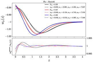
Figure 1: Upper frame: Geometric dark energy equation of state for the Hu-Sawicki model (9) with different values of $\Omega_{m}^{0}$. Solid lines represent the numerical integration of the field equations and their reconstruction (in dashed lines) comes from the best fit by using (12) (JJE parameterization). a) Black is for $\Omega_{m}^{0}=0.20$, b) Red is for $\Omega_{m}^{0}=0.25$ and c) Blue is for $\Omega_{m}^{0}=0.30$. Best fit parameters are shown in the plot for each case. Bottom frame: Evolution of the ratio parameterized $\omega_{X,param}$ and numerical EoS $\omega_{X}$, values remains within $0.5$%.

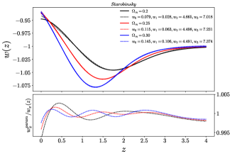
Figure 2: Upper frame: Same as figure [1] for the Starobinsky model (10). Bottom frame: Same as bottom frame in [1]

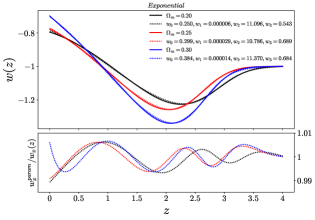
Figure 3: Upper frame: Same as figure [1] for the Exponential model (11). Bottom frame: Same as bottom frame in [1] but, in this case, best fits are within $1$%

IV JJE implementation to observational data.

Given that we are interested in modelling the late-time evolution of the universe we use observational data from BAO redshift surveys, SNeIA luminous distance from Union 2.1 union21 and the latest high-z measurements of $H(z)$ from Cosmic Chronometers cc .

We use measurements of the BAO peak from the galaxy redshift surveys six-degree-field galaxy survey (6dFGS Beutler:2011hx ), Sloan Digital Sky Survey Data Release 7 (SDSS DR7 Ross:2014qpa ) and the reconstructed value (SDSS(R) Padmanabhan2pc ), as well as the latest result from the complete BOSS sample SDSS DR12 (Alam:2016hwk ), and also from the Lyman-$\alpha$ Forest measurements from the Baryon Oscillation Spectroscopic Data Release 11 (BOSS DR11 Font-Ribera:2013wce , Delubac:2014aqe ). Since the volume surveyed by BOSS and WiggleZ Kazin:2014qga partially overlap we do not use data from the latter in this work (see details in Beutler:2015tla ). Even though the current supernovae compilation is given by the JLA sample Betoule:2014frx , in this work we implement the Union 2.1 sample since the apparent magnitude ratio is less than $0.2\%$ in the redshift range of our interest (above $z=1$) in comparison to the JLA sample.

In addition to the free parameters in (12) we vary the fractional amount of matter $\Omega_{M}$ and the value of $H_{0}$, by means of a standard $\chi^{2}$ approach we find the constraints at 1 and 2-$\sigma$ level.

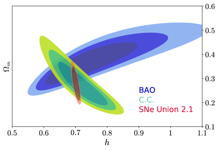
Figure 4: Constraints on the $\Omega_{M}$-$h$ space for the JJE parametrization (12).

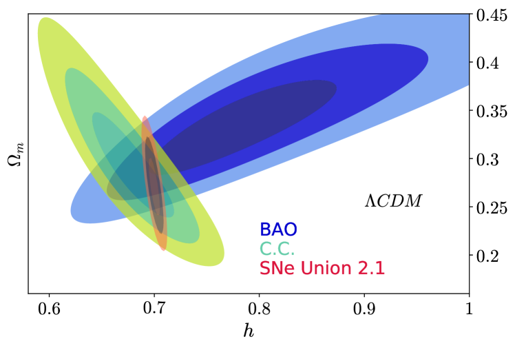
Figure 5: Constraints on the $\Omega_{M}$-$h$ space for $\Lambda$CDM model.

In Figures (4) and (5) we notice that the constraints on
$\Omega_{M}$-$h$ parameter space are tighter for $\Lambda$CDM scenario in comparison with the JJE parameterisation. As for the contours at 1-$\sigma$ from the different datasets it is noticeable that they do overlap for the JJE parameterisation while a tension with ${\Delta\chi^{2}}_{\text{reduced (SN-BAO)}}=0.961$ and ${\Delta\chi^{2}}_{\text{reduced (CC-BAO)}}=0.348$ is present among the BAO and supernovae results when $\Lambda$CDM is assumed.

To compare our JJE model with $\Lambda$CDM we use the combination of the three different datasets (SN+BAO+CC) and calculate the corresponding reduced-$\chi^{2}$ estimator by taking into account the different number of degrees of freedom among the two models. From the obtained values we find that JJE parameterisation and $\Lambda$CDM are consistent showing a difference of $\Delta\chi^{2}_{\text{reduced}(\text{JJE}-\Lambda\text{CDM})}=0.5\%$.

V Discussion.

The scientific community is devoting a large amount of time and resources in the quest to understand the dynamics and nature of dark energy, working on current (SDSS-IV Dawson:2015wdb , DES Abbott:2005bi ) and future (DESI Levi:2013gra ; Aghamousa:2016zmz , Euclid 2011arXiv1110.3193L , LSST 2009arXiv0912.0201 ) experiments to study with very high precision the expansion history of the universe and thus be able to test interesting theoretical models. In the process of analyzing data coming, for instance, from galaxy redshift surveys, a cosmological model is used throughout the pipeline (RSD-paper ). Also, analysis of the CPL parameterisation using forecast for the eBOSS has been done in Ruggeri:2017rza to convert observed positions of the objects into coordinates.

Therefore, to implement in an easy and efficient way modified gravity theories in any kind of survey, we proposed the JJE parameterisation (12). Similarly, in future forecast analysis (DESI-forecasting ) a cosmological model will be needed to investigate the parameter constraints in modified gravity theories.

With the presented proposal we aim to put theoretical background to parameterizations of $\omega_{X}$ and also models for $f(R)$ gravity at the same level as other parameterisations into the pipeline and analysis of observational data and forecasts.

It is worth to mention that by introducing this parameterisation in surveys or using it for data analysis we are avoiding any other kind of assumption that are usually taken in $f(R)$. One of the most usual assumptions is the one related to the value of $f_{R}(z=0)$  which is taken very close to $1$ because of the Solar System constrains Hu:2007nk or the structure formation EXP . Nevertheless it is important to notice this constrictions are usually computed for the Hu-Sawicki model and such values do not necessarily apply to other models. By using the JJE parametrization we are making no assumption whatsoever over such values.

Acknowledgements.- The Authors thanks to M. Zumalacarregui for taking the time of reading these ideas and give us fruitful feedback. C.E-R. acknowledges MCTP-UNACH. M.J. thanks to CONACyT for the PhD fellowship.

References

- (1) A. G. Riess et al. [Supernova Search Team Collaboration], Astron. J. 116, 1009 1998 [astro-ph/9805201]. S. Perlmutter et al. [Supernova Cosmology Project Collaboration], Astrophys. J. 517, 565 1999 Available online: [astro-ph/9812133].
- (2) D. J. Eisenstein et al. [SDSS Collaboration], Astrophys. J. 633, 560 2005 Available online: [astro-ph/0501171].
- (3) D. N. Spergel et al. [WMAP Collaboration], Astrophys. J. Suppl. 148, 175 2003 Available online: [astro-ph/0302209].
- (4) M. Tegmark et al. [SDSS Collaboration], Phys. Rev. D 69, 103501 2004 Available online: [astro-ph/0310723].
- (5) B. Jain and A. Taylor, Phys. Rev. Lett. 91, 141302 2003 Available online: [astro-ph/0306046].
- (6) R. Laureijs et al. [EUCLID Collaboration], ESA/SRE 201112 Available online: arXiv:1110.3193 [astro-ph.CO]. L. Amendola et al. [Euclid Theory Working Group Collaboration], Living Rev. Rel. 16, 6 2013 Available online: [arXiv:1206.1225 [astro-ph.CO]]. L. Samushia et al., Mon. Not. Roy. Astron. Soc. 439, no. 4, 3504 2014 Available online: [arXiv:1312.4899 [astro-ph.CO]]. F. Abdalla et al., FERMILAB-TM-2547-AE 2012 Available online: arXiv:1209.2451 [astro-ph.CO]. Myers, S. T., Abdalla, F. B., Blake, C., Koopmans, L., Lazio, J., and Rawling, S. 2009, Vol. 2010, Astro2010: The Astronomy and Astrophysics Decadal Survey, 219, Available online: [arXiv:0903.0615].
- (7) Delubac, Timothy et al doi:10.1051/0004-6361/201423969
- (8) P. A. R. Ade et al. [Planck Collaboration], Astron. Astrophys. 594, A13 (2016) doi:10.1051/0004-6361/201525830
- (9) A. G. Riess et al., Astrophys. J. 826, no. 1, 56 (2016) doi:10.3847/0004-637X/826/1/56 [arXiv:1604.01424 [astro-ph.CO]].
- (10) S. Alam et al. [BOSS Collaboration], Mon. Not. Roy. Astron. Soc. 470, no. 3, 2617 (2017) doi:10.1093/mnras/stx721
- (11) B. P. Abbott et al. [LIGO Scientific and Virgo and 1M2H and Dark Energy Camera GW-E and DES and DLT40 and Las Cumbres Observatory and VINROUGE and MASTER Collaborations], Nature 551, no. 7678, 85 (2017) doi:10.1038/nature24471
- (12) G. B. Zhao et al., Nat. Astron. 1 (2017) 627 doi:10.1038/s41550-017-0216-z [arXiv:1701.08165 [astro-ph.CO]].
- (13) A. Shafieloo, V. Sahni and A. A. Starobinsky, Phys. Rev. D 86, 103527 (2012) doi:10.1103/PhysRevD.86.103527 [arXiv:1205.2870 [astro-ph.CO]].
- (14) L. G. Jaime, L. Patiño and M. Salgado, Phys. Rev. D 89, no. 8, 084010 (2014) doi:10.1103/PhysRevD.89.084010 [arXiv:1312.5428 [gr-qc]].
- (15) A. Barreira, B. Li, C. Baugh and S. Pascoli, JCAP 1408, 059 (2014) doi:10.1088/1475-7516/2014/08/059 [arXiv:1406.0485 [astro-ph.CO]].
- (16) K. S. Kumar, J. C. Bueno Sánchez, C. Escamilla-Rivera, J. Marto and P. Vargas Moniz, JCAP 1602, no. 02, 063 (2016) doi:10.1088/1475-7516/2016/02/063 [arXiv:1504.01348 [astro-ph.CO]].
- (17) J. Renk, M. Zumalacárregui, F. Montanari and A. Barreira, JCAP 1710, no. 10, 020 (2017) doi:10.1088/1475-7516/2017/10/020 [arXiv:1707.02263 [astro-ph.CO]].
- (18) J. M. Ezquiaga and M. Zumalacárregui, Phys. Rev. Lett. 119, no. 25, 251304 (2017) doi:10.1103/PhysRevLett.119.251304 [arXiv:1710.05901 [astro-ph.CO]].
- (19) Chevallier, Michel and Polarski, David, International Journal of Modern Physics D 10, 213 (2001). doi:10.1142/S0218271801000822
- (20) Linder, Eric V. Phys. Rev. Lett. 90, 091301 (2003) doi:10.1103/PhysRevLett.90.091301
- (21) Laureijs, R. et al. ESA/SRE(2011)12 arXiv:1110.3193 [astro-ph.CO]
- (22) M. Levi et al. [DESI Collaboration], arXiv:1308.0847 [astro-ph.CO].
- (23) A. Aghamousa et al. [DESI Collaboration], arXiv:1611.00036 [astro-ph.IM].
- (24) L. G. Jaime, L. Patino and M. Salgado, Phys. Rev. D 83, 024039 (2011) doi:10.1103/PhysRevD.83.024039
- (25) L. G. Jaime, Phys. Rev. D 91, no. 12, 124070 (2015) doi:10.1103/PhysRevD.91.124070 [arXiv:1506.03618 [gr-qc]].
- (26) E. Berti et al., Class. Quant. Grav. 32, 243001 (2015) doi:10.1088/0264-9381/32/24/243001 [arXiv:1501.07274 [gr-qc]].
- (27) W. Hu and I. Sawicki, Phys. Rev. D 76, 064004 (2007) doi:10.1103/PhysRevD.76.064004
- (28) A. A. Starobinsky, JETP Lett. 86, 157 (2007) doi:10.1134/S0021364007150027
- (29) E. V. Linder, Phys. Rev. D 80, 123528 (2009) doi:10.1103/PhysRevD.80.123528 [arXiv:0905.2962 [astro-ph.CO]]. L. G. Jaime and M. Salgado, arXiv:1711.08026 [gr-qc]. S. D. Odintsov, D. Sáez-Chillón Gómez and G. S. Sharov, Eur. Phys. J. C 77, no. 12, 862 (2017) doi:10.1140/epjc/s10052-017-5419-z [arXiv:1709.06800 [gr-qc]].
- (30) L. G. Jaime, L. Patino and M. Salgado, arXiv:1206.1642 [gr-qc].
- (31) M. Zumalacárregui, E. Bellini, I. Sawicki, J. Lesgourgues and P. G. Ferreira, JCAP 1708, no. 08, 019 (2017) doi:10.1088/1475-7516/2017/08/019 [arXiv:1605.06102 [astro-ph.CO]].
- (32) C. Escamilla-Rivera, Galaxies 4, no. 3, 8 (2016) doi:10.3390/galaxies4030008
- (33) M. Jaber and A. de la Macorra, Astropart. Phys. 97, 130 (2018) doi:10.1016/j.astropartphys.2017.11.007 [arXiv:1708.08529 [astro-ph.CO]].
- (34) Y. Wang et al. [BOSS Collaboration], Mon. Not. Roy. Astron. Soc. 469, no. 3, 3762 (2017) doi:10.1093/mnras/stx1090 [arXiv:1607.03154 [astro-ph.CO]].
- (35) http://desi.lbl.gov/wp-content/uploads/2014/04/fdr-science-biblatex.pdf
- (36) Suzuki, N. ApJ 746, 85 (2012) doi: 10.1088/0004-637X/746/1/85 [arXiv:1105.3470]
- (37) M. Moresco et al., JCAP 1605, no. 05, 014 (2016) doi:10.1088/1475-7516/2016/05/014 [arXiv:1601.01701 [astro-ph.CO]].
- (38) Beutler, F. and Blake, C. and Colless, M. and Jones, D. H. and Staveley-Smith, L. and Campbell, L. and Parker, Q. and Saunders, W. and Watson, F., doi :10.1111/j.1365-2966.2011.19250.x
- (39) Ross, Ashley J. and Samushia, Lado and Howlett, Cullan and Percival, Will J. and Burden, Angela and Manera, Marc, Mon. Not. Roy. Astron. Soc. 449 (2015) 1, 835-847, doi:10.1093/mnras/stv154
- (40) Padmanabhan, Nikhil and Xu, Xiaoying and Eisenstein, Daniel J. and Scalzo, Richard and Cuesta, Antonio J. and Mehta, Kushal T. and Kazin, Eyal, Mon. Not. Roy. Astron. Soc. 427 doi:10.1111/j.1365-2966.2012.21888.x
- (41) Font-Ribera, Andreu and others, doi:10.1088/1475-7516/2014/05/027
- (42) Kazin, Eyal A. and others, doi:10.1093/mnras/stu778
- (43) Beutler, Florian and Blake, Chris and Koda, Jun and Marin, Felipe and Seo, Hee-Jong and Cuesta, Antonio J. and Schneider, Donald P., doi:10.1093/mnras/stv1943
- (44) M. Betoule et al. [SDSS Collaboration], Astron. Astrophys. 568, A22 (2014) doi:10.1051/0004-6361/201423413 [arXiv:1401.4064 [astro-ph.CO]].
- (45) Dawson, Kyle S. and others doi:10.3847/0004-6256/151/2/44
- (46) Abbott, T. and others ”The dark energy survey”, astro-ph/0510346”
- (47) LSST Science Collaboration and Abell, P. A. and Allison, J. and Anderson, S. F. and Andrew, J. R. and Angel, J. R. P. and Armus, L. and Arnett, D. and Asztalos, S. J. and Axelrod, T. S. and et al. arXiv:0912.0201
- (48) A. Ferté, D. Kirk, A. R. Liddle and J. Zuntz, arXiv:1712.01846 [astro-ph.CO]. R. R. W. J. Percival et al., arXiv:1801.02891 [astro-ph.CO].
- (49) R. Ruggeri, W. J. Percival, E. M. Mueller, H. Gil-Marin, F. Zhu, N. Padmanabhan and G. B. Zhao, arXiv:1712.03997 [astro-ph.CO].
- (50) http://desi.lbl.gov/tdr/ http://desi.lbl.gov/wp-content/uploads/2014/04/fdr-science-biblatex.pdf
- (51) L.G. Jaime, M. Jaber and C. Escamilla. In process (2018).