Spin Transport in Half-Metallic Ferromagnet-Superconductor Junctions

Abstract

We investigate the charge and spin transport in half-metallic ferromagnet ($F$) and superconductor ($S$) nanojunctions. We utilize a self-consistent microscopic method that can accommodate the broad range of energy scales present, and ensures proximity effects that account for the interactions at the interfaces are accurately determined. Two experimentally relevant half-metallic junction types are considered: The first is a $F_{1}F_{2}S$ structure, where a half-metallic ferromagnet $F_{1}$ adjoins a weaker conventional ferromagnet $F_{2}$. The current is injected through the $F_{1}$ layer by means of an applied bias voltage. The second configuration involves a $SF_{1}F_{2}F_{3}S$ Josephson junction whereby a phase difference $\Delta\varphi$ between the two superconducting electrodes generates the supercurrent flow. In this case, the central half-metallic $F_{2}$ layer is surrounded by two weak ferromagnets $F_{1}$ and $F_{3}$. By placing a ferromagnet with a weak exchange field adjacent to an $S$ layer, we are able to optimize the conversion process in which opposite-spin triplet pairs are converted into equal-spin triplet pairs that propagate deep into the half-metallic regions in both junction types. For the tunnel junctions, we study the bias-induced local magnetization, spin currents, and spin transfer torques for various orientations of the relative magnetization angle $\theta$ in the $F$ layers. We find that the bias-induced equal-spin triplet pairs are maximized in the half-metal for $\theta\approx 90^{\circ}$ and as part of the conversion process, are anticorrelated with the opposite-spin pairs. We show that the charge current density is maximized, corresponding to the occurrence of a large amplitude of equal-spin triplet pairs, when the exchange interaction of the weak ferromagnet is about $0.1E_{F}.$ For the half-metallic Josephson junctions we often find that the spin current flowing in the half-metal is equivalent to the charge supercurrent flowing throughout the junction. This is indicative that the current consists of spin-polarized triplet pairs. The conversion process of the opposite-spin triplet pairs to the equal-spin triplet pairs in the weaker magnets is clearly demonstrated. This is exemplified by the fact that the supercurrent in the half metal was found to be relatively insensitive to its thickness.

I Introduction

Superconductor ($S$) and ferromagnet ($F$) hybrids have opened up many new possibilities for further advancements in spintronics devices whose purpose is to manipulate the flow of charge and spin currents linder . Central to their functionality is experimental control of the spin degree of freedom while enjoying the dissipationless nature of supercurrent. This control is typically afforded through magnetization rotations of one of the free ferromagnetic layers, achieved via weak in-plane external magnetic fields, or by the spin transfer torque (STT) effect. The most commonly studied transport structures based on superconductors and ferromagnets are equilibrium Josephson junctions or voltage biased superconducting tunnel junctions. In any case, the underlying junction architecture often involves spin and charge transport through a spin-valve configuration. A basic superconducting spin-valve consists of two or more ferromagnets adjacent to a superconductoroh , where rotation of one of the $F$ layer magnetizations modifies the induced oscillatory singlet pairing in the ferromagnets. If the $F$ layers are half-metallic, these oscillations rapidly dampen out due to their incompatible nature. If however the ferromagnetic regions have non-collinear magnetizations, as will be discussed shortly, triplet pairsberger with parallel projection of spin can be created that extend deep within the half-metal. These spin-polarized triplet pairs are thus of great interest, and their signatures have been experimentally observed in the superconducting critical temperature of half-metallic spin valvesrobby when rotating one of the $F$ layer magnetizations. Transport measurements in a half-metallic Josephson junction keizer demonstrated a supercurrent through the half-metal $\rm CrO_{2}$, also indicating the current is carried by equal-spin Cooper pairs since singlet pairs are blocked by the half metal. Because control of the transport of dissipationless spin-currents is a major objective of low-temperature spintronics devices, superconducting junctions that merge half-metallic ferromagnets and superconductors are increasingly being recognized as valuable platforms to study these two competing orders.

Spin currents can flow within superconducting junctions with two or more $F$ layers due to the ferromagnetic exchange interactions. They can also flow with the help of induced equal-spin triplet pairing correlations, where the Cooper pairs have a net spin of $m=\pm 1$ on the spin quantization axis. The generation of these long-range triplet correlations in superconducting heterostructures with magnetic inhomogeneities has been well studied theoretically and experimentally. By introducing magnetic inhomogeneity, e.g., inclusion of multiple magnets with misaligned exchange fields, the Hamiltonian no longer commutes with the total spin operator and equal-spin triplet correlations can be induced. Due to the imbalance between majority and minority spins in a ferromagnet, conventional singlet pairing correlations decay over short distances within the magnetic region. However, Cooper pairs with electrons that carry the same spin ($m=\pm 1$) are not subject to the paramagnetic pair breaking and can in principle propagate for large distances inside the ferromagnet, limited only by coherence breaking processes. Such long-range $m=\pm 1$ triplet correlations thus play an important role in Josephson and tunneling junctions containing ferromagnets with noncollinear magnetizations.

While there has been extensive work towards isolating and detecting the triplet pairing state, it can be difficult to disentangle the equal-spin triplet and opposite-spin singlet and triplet correlations. It is therefore of interest to investigate heterostructures that restrict the formation of opposite spin pairs while retaining the desired equal-spin triplet correlations. The pinpointing of triplet effects can be exploited with the use of highly polarized materials like half metallic ferromagnets, where only a single spin channel is present at the Fermi level. The ordinary singlet pairs and opposite-spin triplet pairs are consequently suppressed, as the magnet behaves essentially as an insulator for the opposite spin band. Half-metallic ferromagnets are thus finding increasing use in superconducting spin valves ah18 . Several half metallic materials are considered in connection with superconducting hybridskriv and spintronic applications. These include the manganese perovskite ${\rm La_{2/3}Ca_{1/3}MnO_{3}}$, as well as the Heusler compounds such as $\rm Cu_{2}MnAl$, which are favorable experimentally, since they can be grown by sputtering techniques sprungmann . The conducting ferromagnet $\rm CrO_{2}$ singh is also a candidate for use in half-metallic spin valves, although it cannot be grown by sputtering methods, and is metastable.

Experimental signatures of triplet correlations in half-metallic $SF_{1}F_{2}$ spin valves have been demonstrated in transition temperature $T_{c}$ variations that occur when rotating the magnetization of the free ferromagnet layer. singh ; robby Measuring the corresponding maximal change in the critical temperature, $\Delta T_{c}$, can represent the emergence of spin-polarized triplet pairs as the singlet superconducting state weakens and is subsequently converted into opposite-spin and equal-spin triplet pairs. Most experiments for these types of spin valve structures involved weak ferromagnets for the outer $F_{2}$ layer and in-plane magnetic fields, yielding $\Delta T_{c}$ sensitivities from a few mK to around 100 mK. zhu ; lek ; wang ; ilya ; flok When the $F_{2}$ layer is replaced by a the half-metallic ferromagnet such as $\rm CrO_{2}$, a larger $\Delta T_{c}$ of $\Delta T_{c}\approx 800\,{\rm mK}$ was measuredsingh using a large out-of-plane applied magnetic field. If $\rm La_{0.6}Ca_{0.4}MnO_{3}$ is used as the half metallic ferromagnet, a much weaker in-plane magnetic field suffices to rotate the magnetization in one of the $F$ layers robby , resulting $\Delta T_{c}\approx 150\,\rm{mK}$, which again is a stronger spin valve effect compared to experiments involving standard ferromagnets lek ; wang . These types of improvements were shown to be consistent with theoretical workhmkh which demonstrated that when the exchange field in $F_{2}$ varies from zero to half-metallic, the largest $\Delta T_{c}$ arises when $F_{2}$ is a half-metallic. These experimental evidences further established the advantages of utilizing half-metallic elements in superconducting spintronics devices.

Although critical temperature measurements give valuable information regarding half-metallic spin valves, for spintronics devices it is important to also investigate the transport of charge and spin in these types of spin-valve structures. By placing the spin valve between two superconducting banks with a phase difference $\Delta\varphi$, a half-metallic based Josephson junction with spin-controlled supercurrent can be generated. Interest in Josephson junctions with ferromagnetic layers has grown due to their use in cryogenic spintronic systems, including superconducting computers and nonvolatile memories,eshy ; effy ; golubov ; buzdin1 where their use in single flux quantum circuits can improve switching speeds.giaz ; spath ; ali To determine whether Josephson structures can serve as viable spintronic devices, it is crucial to understand the behavior of the spin currents that can flow in such systems. The interaction between the spin currents and the magnetizations in ferromagnetic Josephson junctions is important for memory applications since the magnetization orientations in the $F$ layers dictates the storage of information bits. Controlling the magnetization rotation can be achieved by a torque from the spin-polarized currents flowing perpendicular to the layers. Some of the spin angular momentum of the polarized current will be transferred to the ferromagnets, giving rise to the STT effect slon ; bergerl ; linder ; linder2 ; sac ; sstech . This effect can result in a decrease of magnetization switching times in random access memories fart ; brataas_nat ; Bauer_nat . The STT effect is known to occur in a broad variety of ferromagnetic materials, including half-metals, making it widely accessible experimentally.

An essential mechanism responsible for supercurrent flow in a half-metallic Josephson junction is Andreev reflection that occurs at the ferromagnet and superconductor interfaces.radovic2 ; radovic1 ; beenaker2 ; beenaker1 In addition to continuum states, the superposition of localized quasiparticle wavefunctions in the ferromagnet regions results in subgap bound states that contribute to the total current flow. For strong ferromagnets, the corresponding spin-polarized Andreev bound states can be strongly affected by the supercurrent, directly influencing the spin currents and STT when varying the relative in-plane magnetization angle. Although the charge current is conserved, remaining uniform throughout the sample, the spin current often varies spatially, making comparisons between the two types of current difficult. Moreover, since manipulating the angle between the magnetization vectors can generate long ranged spin polarized triplet supercurrents hvw15 , these triplet correlations also correlate with spatial variations in the spin currents responsible for the mutual torques acting on the ferromagnets.

As demonstrated in Refs. robinson, ; khaire, , these equal-spin triplet pairs result in a more robust Josephson supercurrent that is relatively insensitive to $F$ layer thicknesses due to their long-ranged nature. If one of the ferromagnets in the junction is half-metallic, the equal-spin triplet correlations are expected to play an even greater role in the behavior of the charge and spin currents. This was shown experimentallykeizer where a spin triplet supercurrent was measured through the half-metal $\rm CrO_{2}$, and whose direction was switchable via magnetization variation. Even in the diffusive limit, it was shown that spin-flip scattering events at the interfaces of a half-metallic Josephson junction also allow penetration of the equal-spin pairs into the half-metal gobu . Considering the potentially greater control of spin currents afforded by Josephson junctions with strongly spin-polarized ferromagnets, it would be illuminating to systematically investigate the interplay of the triplet pair correlations with the charge and spin transport throughout half-metallic Josephson structures.

Another way to produce charge and spin currents in half-metallic spin valve structures involves establishing a voltage difference between the ends of a $F_{1}F_{2}S$ tunnel junction, resulting in an injected current into the $F_{1}$ layer. The charge and spin transport properties for these types of nonequilibrium tunnel junctions with relatively weak ferromagnets was previously studied wvh14 ; mv17 as functions of bias voltage using a transfer matrix approach that combines the Blonder-Tinkham-Klapwijk (BTK) formalism and self-consistent solutions to the Bogolibuov-de Gennes (BdG) equations. The use of this technique was also extended to accurately compute spin transport quantities, including STT and the spin currents, while ensuring that the appropriate conservation laws are satisfied. If the $F_{1}$ layer is half-metallic, the current can become strongly polarized, leading to a relatively large transfer of angular momentum to the $F_{2}$ layer for noncollinear magnetizations, via the STT effect. Also, the angularly averaged subgap conductance in this case arises mainly from anomalous Andreev reflection wvh14 , whereby a reflected hole with the same spin as the incident particle is Andreev reflected, generating a spin-polarized triplet pair. The effects of applied bias on the spin transfer torque and the spin-polarized tunneling conductance has also been previously studied in superconducting tunnel junctions linder0 . By applying an external magnetic field, or through switching via STT, it is again possible to control the relative orientation of the intrinsic magnetizations and investigate the dependence of the charge and spin currents on the misorientation angle $\theta$ between the two ferromagnetic layers. Thus, when a half-metallic layer is present in a $F_{1}F_{2}S$ tunnel junction, we can have greater control and isolation of the spin currents and spin-polarized triplet pairs that are critical for viable spintronics platforms. The systematic investigation into the transport and corresponding triplet correlations of half-metallic spin valves for both equilibrium Josephson junctions and nonequilibrium tunnel junctions is the main focus of this paper.

When considering spin transport in superconducting junctions, it is beneficial for the structure to contain both weakly polarized and strongly polarized ferromagnets. This is because the singlet and the opposite spin triplet correlations in weaker ferromagnets extend over greater lengths, dictated by the inverse of the exchange field, and they are therefore much more effective at hosting opposite-spin pairs. The weak ferromagnet serves as an intermediate layer between the superconductor and half-metal, facilitating the generation of opposite-spin pairs that will eventually become converted into the longer ranged equal-spin triplet pairs. A hybrid ferromagnetic setup also creates an avenue for the systematic investigation into the interplay and ultimate control of both triplet channels. We therefore are interested in two types of tunnel junctions in this paper. The first consists of a single superconductor in contact with two ferromagnets (an $F_{1}F_{2}S$ structure), with the $F_{2}$ ferromagnet having a weak exchange field, and the other $F_{1}$, half-metallic. The current in this nonequilibrium case is injected by means of a voltage difference between two electrodes. As alluded to earlier, the other scenario involves a Josephson junction containing a half-metal flanked by two weaker conventional ferromagnets. The current is established in the usual way by a macroscopic phase difference $\Delta\varphi$ between the two outer superconducting banks. For both junction arrangements, we investigate the charge and spin transport within the ballistic regime using a microscopic self-consistent BdG formalism that is capable of accommodating the broad range of energy scales set by the exchange field $h$ of the conventional ferromagnets ($h/E_{F}\ll 1$) and the half-metal ($h=E_{F}$). Of crucial importance towards the theoretical description of these type of transport structures is to accurately be able to account for the mutual interactions between the ferromagnetic and superconducting elements, i.e., proximity effects. This requires a self-consistent treatment, which ensures that the final solutions minimize the free energy of the system and satisfies the proper conservation laws. This numerical approach is a time-consuming but necessary step to reveal the self-content proximity effects that govern the nontrivial charge and spin currents that flow within these structures. Indeed, the tunneling conductance in $F_{1}F_{2}S$ junctions was shown to differ substantially from that obtained via a non-self-consistent approach wvh14 .

This paper is organized as follows: In Sec. II.1, we present the general Hamiltonian and self-consistent BdG methodology that is applicable for both junction configurations. In Sec. II.2, the transfer matrix approach for tunnel junctions that combines the Blonder-Tinkham-Klapwijk (BTK) formalism and self-consistent solutions to the BdG equations is established. The charge continuity equation and current density are also derived. In Sec. II.3, the relevant details for the characterization of equilibrium half-metallic Josephson junctions and the expression for the associated current density are given. In Sec. II.4, we outline how to calculate the induced triplet correlations for equilibrium Josephson junctions and non-equilibrium tunnel junctions. In Sec. II.5 the techniques used to compute the spin transport quantities including magnetization, spin-transfer torque, and the spin current are derived for both types of junctions. Throughout Sec. II, we discuss how to properly satisfy the conservation laws for charge and spin densities in our formalism. In Sec. III.1 we present the results for half-metallic tunnel junctions. Results for the spatial dependence to the bias-induced magnetizations, the spin-transfer torque, the spin currents, and triplet correlations are presented as functions of the magnetization misalignment angle as well as the applied bias. We also report how to take advantage of the induced triplet correlations by choosing the optimal exchange interactions in $F$ layers. In Sec. III.2, we present the results for the half-metallic Josephson junctions, including the current phase relations for a variety of half-metal thicknesses. The spatial dependencies to the spin currents and triplet correlations are given, and a broad range of misalignment angles are considered to demonstrate the propagation of spin-polarized triplet pairs through the half-metal. The positive correlations between the equal-spin triplet correlations and the spin-polarized supercurrents are also discussed. We conclude with a summary in Sec. IV.

II Methods

II.1 Description of the systems

Two types of half-metallic junctions are considered in this paper: tunneling junctions and Josephson junctions. The effective Hamiltonian that is applicable to both types of junctions is

$${\cal H}_{\rm eff} = \int d^{3}r\left\{\sum_{s}\psi_{s}^{\dagger}\left(\bm{r}\right)H_{0}\psi_{s}\left(\bm{r}\right)\right.$$ (1)

$$+ \left.\frac{1}{2}\left[\sum_{s\>s^{\prime}}\left(i\sigma_{y}\right)_{ss^{\prime}}\Delta\left(\bm{r}\right)\psi_{s}^{\dagger}\left(\bm{r}\right)\psi_{s^{\prime}}^{\dagger}\left(\bm{r}\right)+H.c.\right]\right.$$

$$- \left.\sum_{s\>s^{\prime}}\psi_{s}^{\dagger}\left(\bm{r}\right)\left(\bm{h}\cdot\bm{\sigma}\right)_{ss^{\prime}}\psi_{s^{\prime}}\left(\bm{r}\right)\right\},$$

where $H_{0}$ is the single-particle part of ${\cal H}_{\rm eff}$, $\bm{h}$ describes exchange interaction of the magnetism, $s$ and $s^{\prime}$ are spin indices and $\bm{\sigma}$ are Pauli matrices. $\Delta(\bm{r})\equiv g\left(\bm{r}\right)\left\langle\psi_{\uparrow}\left(\bm{r}\right)\psi_{\downarrow}\left(\bm{r}\right)\right\rangle$ is the superconducting pair potential and $g(\bm{r})$ is the coupling constant. In ferromagnets where there is no intrinsic superconducting pairing, $g(\bm{r})$ is taken to be zero. Similarly, $\bm{h}$ vanishes in intrinsically superconducting regions. Following Ref. wvh14, , we utilize the generalized Bogoliubov transformation bdg , $\psi_{s}=\sum_{n}\left(u_{ns}\gamma_{n}+\eta_{s}v_{ns}^{\ast}\gamma_{n}^{\dagger}\right)$, where $\eta_{s}\equiv 1(-1)$ for spin-down (up), to write down the BdG Hamiltonian equivalent to Eq. (1):

$$\begin{pmatrix}H_{0}-h_{z}&-h_{x}+ih_{y}&0&\Delta\\ -h_{x}+ih_{y}&H_{0}+h_{z}&\Delta&0\\ 0&\Delta&-(H_{0}-h_{z})&-h_{x}+ih_{y}\\ \Delta&0&-h_{x}+ih_{y}&-(H_{0}+h_{z})\\ \end{pmatrix}\begin{pmatrix}u_{n\uparrow}\\ u_{n\downarrow}\\ v_{n\uparrow}\\ v_{n\downarrow}\end{pmatrix}$$

$$=\epsilon_{n}\begin{pmatrix}u_{n\uparrow}\\ u_{n\downarrow}\\ v_{n\uparrow}\\ v_{n\downarrow}\end{pmatrix},$$ (2)

where $u_{ns}$ and $v_{ns}$ in the generalized Bogoliubov transformations can be identified as the quasiparticle and quasihole amplitudes, respectively.

For layered tunnel junctions and Josephson junctions considered in this work, we assume each $F$ and $S$ layer is infinite in the $yz$ plane and the layer thicknesses extend along the $x$ axis (See Figs. 1 and 7). As a result, the BdG Hamiltonian [Eq. (2)] is translationally invariant in the $yz$ plane, and it becomes quasi-one-dimensional in $x$. The single-particle Hamiltonian is $H_{0}=-({1}/{2m})({d^{2}}/{dx^{2}})+{\epsilon_{\perp}}-E_{F}$, where we have defined the transverse kinetic energy as $\epsilon_{\perp}\equiv(k_{y}^{2}+k_{z}^{2})/2m$, and $E_{F}$ denotes the Fermi energy. Although in this work, we do not consider Fermi energy mismatch between distinct layers, it is straightforward to include such an effect. Throughout this paper, we take $\hbar=k_{B}=1$, and all energies are measured in units of $E_{F}$. We numerically determine the pair potential by using fully self-consistent solutions to Eq. (2). The iterative self-consistent procedure has been extensively discussed in previous work wvh12 ; wvh14 . Since our BdG Hamiltonian is quasi-one-dimensional, the pair potential is only a function of $x$. By minimizing the free energy of the system, and making use of the generalized Bogoliubov transformation, the pair potential can be written as,

$$\Delta(x)=\frac{g(x)}{2}{\sum_{n}}^{\prime}\bigl{[}u_{n\uparrow}(x)v_{n\downarrow}^{\ast}(x)+u_{n\downarrow}(x)v_{n\uparrow}^{\ast}(x)\bigr{]}\tanh\left(\frac{\epsilon_{n}}{2T}\right),\,$$ (3)

where $T$ is temperature and the prime symbol means that a Debye cutoff energy, $\omega_{D}$, is introduced in the energy sum. Additional details of our formalism used in this work can also be found in Refs. wvh14, ; hvw15, .

II.2 Tunnel junctions

We begin first with tunnel junctions depicted in Fig. 1 where a ferromagnet and half metal are in contact with a superconductor. The ferromagnet that is not adjacent to $S$ is labeled $F_{1}$, and the one next to $S$ is $F_{2}$. As shown in Fig. 1, the exchange field in $F_{1}$ is $h_{1}\hat{\bm{z}}$, and in $F_{2}$ it is $h_{2}\left(\sin\theta\hat{\bm{y}}+\cos\theta\hat{\bm{z}}\right)$. Here $h_{1}$ and $h_{2}$ are the magnitudes of the exchange fields in $F_{1}$ and $F_{2}$, respectively. In general, we consider $F_{1}$ as a fixed layer where the exchange field is pinned and $F_{2}$ as a free layer where the relative angle $\theta$ can be controlled by an applied magnetic field experimentally ilya . In this work, we take the fixed layer $F_{1}$ to be a half metal and $h_{1}=E_{F}.$

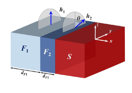
Figure 1: (Color online) Illustration of the ${F_{1}F_{2}S}$ tunnel junction that is infinite and translationally invariant in the $yz$ plane. It has finite size along the $x$ axis. $F_{1}$ is a half-metal and the associated exchange field is fixed along the $z$ direction. The direction of the exchange field in $F_{2}$ is in the $yz$ plane, and makes an angle $\theta$ with the $z$ axis. Such a misorientation can be achieved experimentally via an external magnetic field.

In previous work wvh14 , a formalism based on the BTK approach btk was generalized to study spin-transport quantities. In Ref. btk, , it was shown, starting from the Boltzmann equation, that the conductance associated with the tunnel junction is a function of the transmission and reflection amplitudes in the linear response regime. Therefore, to compute the tunneling conductance, one should start by writing down the appropriate wavefunctions in each distinct region. If one considers a bilayer tunnel junction that is made up of a non-magnetic metal and a superconductor, then the eigenfunctions in the non-magnetic metallic region are only linear combinations of particle and hole wavefunctions.btk However, in our work, where the non-magnetic metallic region is replaced by two ferromagnetic layers, one should consider the spin degree of freedom in addition to the particle-hole nature. Because the exchange field is along $z$ in $F_{1}$, the appropriate eigenfunctions are

$$\begin{pmatrix}e^{\pm ik^{+}_{\uparrow 1}x}\\ 0\\ 0\\ 0\end{pmatrix},\enspace\begin{pmatrix}0\\ e^{\pm ik^{+}_{\downarrow 1}x}\\ 0\\ 0\end{pmatrix},\enspace\begin{pmatrix}0\\ 0\\ e^{\pm ik^{-}_{\uparrow 1}x}\\ 0\end{pmatrix},\enspace\begin{pmatrix}0\\ 0\\ 0\\ e^{\pm ik^{-}_{\downarrow 1}x}\end{pmatrix},$$ (4)

where the subscript 1 denotes the $F_{1}$ regions and the superscript $+$ is for particle-like and $-$ is for hole-like wavefunctions. When the eigenenergy $\epsilon$ is specified, the corresponding wavevectors are given by the following relation

$$k_{s1}^{\pm}=\left[1-\eta_{s}h_{1}\pm\epsilon-k_{\perp}^{2}\right]^{1/2},$$ (5)

where $k_{\perp}^{2}=k_{y}^{2}+k_{z}^{2}$. The incident angle, $\theta_{I}$, relative to the normal of the interface with spin $s$ is related to $k_{\perp}$ and given by the relation, $\tan\theta_{I}=k_{\perp}/k_{s1}^{\pm}$. The reflected angles, $\theta_{R}$, similarly obey $\tan\theta_{R}=k_{\perp}/k_{s1}^{\pm}$. From Eq. (5), it is easy to see that the reflected angles depend on both the spin as well as whether the quasiparticle is particle-like or hole-like. The exchange field in ${F_{2}}$ lies on the $yz$ plane, and it is tilted relative to the $z$-axis by the angle $\theta$. One needs again to use suitable eigenfunctions for both particle and hole branches in ${F_{2}}$. The particle-like wavefunction with spin parallel to the exchange field in ${F_{2}}$ and antiparallel to the exchange field in ${F_{2}}$ are given as

$$\begin{pmatrix}\cos\left(\theta/2\right)\\ \sin\left(\theta/2\right)\\ 0\\ 0\end{pmatrix}e^{\pm ik^{+}_{\uparrow 2}x},\enspace\enspace\begin{pmatrix}-\sin\left(\theta/2\right)\\ \cos\left(\theta/2\right)\\ 0\\ 0\end{pmatrix}e^{\pm ik^{+}_{\downarrow 2}x},\enspace\enspace$$ (6)

respectively. Similarly, the hole-like wavefunction with spin parallel and antiparallel to the exchange field in $F_{2}$ are given by

$$\begin{pmatrix}0\\ 0\\ \cos\left(\theta/2\right)\\ -\sin\left(\theta/2\right)\end{pmatrix}e^{\pm ik^{-}_{\uparrow 2}x},\enspace\enspace\begin{pmatrix}0\\ 0\\ \sin\left(\theta/2\right)\\ \cos\left(\theta/2\right)\end{pmatrix}e^{\pm ik^{-}_{\downarrow 2}x},\enspace\enspace$$ (7)

respectively. Here the momenta are defined through the relation

$$k_{s2}^{\pm}=\left[1-\eta_{s}h_{2}\pm\epsilon-k_{\perp}^{2}\right]^{1/2}.$$ (8)

Note here that following previous conventions, we denote $``+"$ for particles, and $``-"$ for holes. Because the Hamiltonian is translationally invariant in the $yz$ plane, the perpendicular momentum $k_{\perp}$ is a constant throughout the “entire” junction for a given eigenstate appropriate to the entire junction. Once the energy of the eigenstate, $\epsilon$, is prescribed, the eigenfunctions in the $F_{2}$ region are given as a linear combination of these wavefunctions. Accordingly, there are eight unknowns associated with this linear combination. On the superconducting side, one can easily show that in $4\times 4$ Nambu space, the appropriate wavefunctions are

$$\begin{pmatrix}u_{0}\\ 0\\ 0\\ v_{0}\end{pmatrix}e^{\pm ik^{+}x},\enspace\begin{pmatrix}0\\ u_{0}\\ v_{0}\\ 0\end{pmatrix}e^{\pm ik^{+}x},\enspace\begin{pmatrix}v_{0}\\ 0\\ 0\\ u_{0}\end{pmatrix}e^{\pm ik^{-}x},\enspace\begin{pmatrix}0\\ v_{0}\\ u_{0}\\ 0\end{pmatrix}e^{\pm ik^{-}x},$$ (9)

where $k^{\pm}=1\pm\sqrt{\epsilon^{2}-\Delta_{0}^{2}-k_{\perp}^{2}}$. If a non-self-consistent pair potential is adopted for which the pair potential in the $S$ region is a constant, the entire $S$ region is just a linear combination of the above wavefunctions with suitable constants $u_{0}$ and $v_{0}$ given by,

$$u_{0}^{2}= \frac{1}{2}\left(1+\frac{\sqrt{\epsilon^{2}-\Delta_{0}^{2}}}{\epsilon}\right),$$ (10a)

$$v_{0}^{2}= \frac{1}{2}\left(1-\frac{\sqrt{\epsilon^{2}-\Delta_{0}^{2}}}{\epsilon}\right),$$ (10b)

where $\Delta_{0}$ is the constant pair amplitude. Let us first discuss the non-self-consistent case and suppose a spin-up particle is sent from an electrode into the $F_{1}$ region. In the $F_{1}$ region, one needs to include the incident spin-up particle wavefunction as well as four different types of reflection: (1) a reflected particle wavefunction with spin-up, (2) a reflected particle wavefunction with spin-down, (3) an Andreev reflected hole wavefunction with spin-up, and (4) an Andreev reflected hole wavefunction with spin-down. As a result, we have four unknowns associated with these four reflected wavefunctions. In the $F_{2}$ region, all eight possibilities, Eqs. (6) and (7), must be considered, since in general the waves can travel in either the $+x$ or $-x$ directions. In the $S$ region, there are four different types of transmitted wavefunctions: two transmitted particle-like wavefunctions,

$$\begin{pmatrix}u_{0}\\ 0\\ 0\\ v_{0}\end{pmatrix}e^{ik^{+}x},\enspace\begin{pmatrix}0\\ u_{0}\\ v_{0}\\ 0\end{pmatrix}e^{ik^{+}x},\enspace$$ (11)

and two transmitted hole-like wavefunctions,

$$\begin{pmatrix}v_{0}\\ 0\\ 0\\ u_{0}\end{pmatrix}e^{-ik^{-}x},\enspace\begin{pmatrix}0\\ v_{0}\\ u_{0}\\ 0\end{pmatrix}e^{-ik^{-}x}.$$ (12)

Thus, the total number of unknowns in this process is sixteen (four from the reflections, eight associated with the $F_{2}$ region, and four from the transmissions). We have exactly the same number of constraints to solve for these unknowns because there are two interfaces ($F_{1}/F_{2}$ and $F_{2}/S$) at which the continuous conditions of the wavefunction and its derivative must hold when the interfacial barrier is absent.

If one uses a self-consistent profile for the pair amplitude, $\Delta$ is not a constant and it varies with $x$. It is convenient to consider a transfer-matrix approach to take into account the variation of $\Delta$. The details of this approach are presented in Ref. wvh14, and will not be repeated in this paper. Here, we only summarize the outline of this approach. One first divides the $S$ region into a number of small subregions and approximates each subregion by a constant potential. One can then write down suitable wavefunctions in each subregion. Except for the last subregion where there are only four unknowns linked to four types of transmission, there are eight unknowns associated with each subregion, resulting now in an overall greater number of unknowns. By recognizing the fact that unknowns on one side of an interface are related to those on the other side, we can write,

$$\tilde{\mathcal{M}}_{i}x_{i}=\mathcal{M}_{i+1}x_{i+1},$$ (13)

where $i$ is the index of each subregion, $\tilde{\mathcal{M}}_{i}$ and $\mathcal{M}_{i+1}$ are the corresponding matrices determined by matching the boundary conditions, and $x_{i}$ and $x_{i+1}$ are the column vectors composed of the unknowns in the $i$-th and $i+1$-th subregions. By using this recurrence relation, one naturally relates the reflection coefficients in the $F_{1}$ region with the transmission coefficients in the outermost $S$ layer. Once these transmission and reflection coefficients are found, they can be fed back into the recurrence relation to generate solutions in each subregion. The transfer matrix method is advantageous because the size of the matrix equation needed to be solved is much smaller than the number of unknowns, albeit at the cost of multiplying matrices.

The BTK formalism was originally developed to extract the tunneling conductance from transmitted and reflected amplitudes. The formula for spin-dependent conductance, normalized to that of the normal state, in the low temperature regime is given by

$$G_{s}=1+\frac{k^{-}_{\uparrow 1}}{k^{+}_{s1}}|a_{s\uparrow}|^{2}+\frac{k^{-}_{\downarrow 1}}{k^{+}_{s1}}|a_{s\downarrow}|^{2}-\frac{k^{+}_{\uparrow 1}}{k^{+}_{s1}}|b_{s\uparrow}|^{2}-\frac{k^{+}_{\downarrow 1}}{k^{+}_{s1}}|b_{s\downarrow}|^{2},$$ (14)

where $a_{s\uparrow}$ and $a_{s\downarrow}$ are Andreev reflected waves and $b_{s\uparrow}$ and $b_{s\downarrow}$ are normal reflected waves. In the above expression, the subscript $s$ denotes the spin type of the incident wave into the $F_{1}$ region.

In Ref. wvh14, , the BTK formalism has been generalized to study transport quantities such as spin currents and spin transfer torques. By applying the transfer matrix method outlined above, these position dependent quantities can be properly computed. Below, we shall describe the basic ideas behind our approach. From the Heisenberg equation for the charge density $\rho({\bm{r}})$,

$$\frac{\partial}{\partial t}\left\langle\rho({\bm{r}})\right\rangle=i\left\langle\left[{\cal H}_{eff},\rho({\bm{r}})\right]\right\rangle,$$ (15)

it is not difficult to obtain the following continuity condition for the current density ${\bm{J}}$:

$$\frac{\partial}{\partial t}\left\langle\rho(\bm{r})\right\rangle+\nabla\cdot{\bm{J}}=-4e{\rm Im}\left[\Delta({\bm{r}})\left\langle\psi_{\uparrow}^{\dagger}({\bm{r}})\psi_{\downarrow}^{\dagger}({\bm{r}})\right\rangle\right].$$ (16)

When in the steady state, the first term on the left is dropped. Moreover, when the system is in equilibrium without an external bias, one can use the Bogoliubov transformation together with the conservation law for our quasi-one-dimensional system to conveniently write the continuity equation as:

$$\frac{\partial J_{x}(x)}{\partial x}=2e{\rm Im}\left\{\Delta(x)\sum_{n}\left[u_{n\uparrow}^{*}v_{n\downarrow}+u_{n\downarrow}^{*}v_{n\uparrow}\right]\tanh\left(\frac{\epsilon_{n}}{2T}\right)\right\}.$$ (17)

The self-consistency condition, Eq. (3), demands that the right hand side of Eq. (17) vanishes and that the current is a constant throughout the junction, as expected.

Now consider a non-zero bias, $V$, across the electrodes of a $F_{1}F_{2}S$ junction. The bias generates a non-equilibrium quasi-particle distribution. In the excitation picture, it is clear that all states with energies $\epsilon<eV$ incident from the electrode in $F_{1}$ to the electrode in $S$ should be taken into account in the low $T$ limit wvh14 . Hence, the charge density and the current density can be derived, and are given by:

$$\rho =-e\sum_{ns}|v_{ns}|^{2}-e\sum_{\epsilon_{\bm{k}}<eV}\sum_{s}\left(|u_{{\bm{k}}s}|^{2}-|v_{{\bm{k}}s}|^{2}\right),$$ (18)

$$J_{x} =-\frac{e}{m}{\rm Im}\left[\sum_{\epsilon_{\bm{k}}<eV}\sum_{s}\left(u_{{\bm{k}}s}^{\ast}\frac{\partial u_{{\bm{k}}s}}{\partial x}+v_{{\bm{k}}s}^{\ast}\frac{\partial v_{{\bm{k}}s}}{\partial x}\right)\right],$$ (19)

where we sum over states labeled by their momenta $\bm{k}$ with energies less than the bias. It is easy to see from the above equations that when $V=0$, $J_{x}=0$, and $\rho$ is just the ground-state charge density, as one would expect. The right hand side of the continuity equation, Eq. (16), with the presence of the bias, becomes $-4e{\rm Im}\left[\Delta\sum_{\epsilon_{\bm{k}}<eV}\left(u_{{\bm{k}}\uparrow}^{\ast}v_{{\bm{k}}\downarrow}+v_{{\bm{k}}\uparrow}u_{{\bm{k}}\downarrow}^{\ast}\right)\right]$. We emphasize here that $\Delta$ vanishes in the intrinsically non-superconducting region since the coupling constant is taken to be zero there. Hence, on the $F$ side the spatial derivative of the current vanishes and the current is a constant. On the $S$ side, where $\Delta$ exists, the derivative of the current does not vanish. This does not mean that the conservation law is violated. The right-hand-side actually describes the process of interchange between the quasi-particle current density and the supercurrent density, as clearly discussed in Ref. btk, ; wvh14, .

II.3 Josephson junctions

We next discuss the pertinent aspects of the half-metallic Josephson junctions that we shall investigate. As shown in Fig. 7, we consider $S_{1}F_{1}F_{2}F_{3}S_{2}$ type junctions, where the central half-metallic layer $F_{2}$ is surrounded by two ferromagnets $F_{1}$ and $F_{3}$. We will show below in Sec. III.2 that it is important for the ferromagnets to be thin (relative to $\xi_{F}$, the superconducting proximity length) and for them to have relatively weak exchange fields so that their placement near the superconducting banks allows for the generation of triplet correlations and the associated phase coherent transport. The exchange fields in each of the junction layers reside in-plane and are written

$$\bm{h}_{i}=h_{i}(\sin\theta_{i}\hat{\bm{y}}+\cos\theta_{i}\hat{\bm{z}}),\quad\text{for $i=1,2,3$}.$$ (20)

To compute the dc Josephson current where the bias across the junction is absent, we again numerically look for solutions by iteratively solving Eq. (2), which is very general and can be applied to both the $F_{1}F_{2}S$ tunneling and $S_{1}F_{1}F_{2}S_{2}$ Josephson junctions. Since we wish to determine the current-phase relation for the Josephson junctions, the initial input for the pairing potential is taken to be the bulk gap, $\Delta_{0}$, in ${S_{1}}$ and $\Delta_{0}\exp(i\Delta\varphi)$ in $S_{2}$. With this input, Eq. (2) is then numerically diagonalized and the new pair potential, $\Delta(x)$ is computed from Eq. (3) throughout the entire junction except for small regions (around one coherence length, $\xi_{0}$, from the sample edges) considered as boundaries of the junctions. In these regions, the pair potential is fixed to its bulk absolute value, with phases $0$ and $\Delta\varphi$, respectively. The newly yielded $\Delta(x)$ is then used in the BdG equations and the above process is repeated iteratively until convergence is achieved. From Eq. (16), when current is flowing through the junction, the self-consistently calculated regions are always found to possess the necessary spatially constant current. The important distinction between tunneling and Josephson junctions is the presence of the external bias. For dc Josephson junctions, the bias is absent and the right-hand side of Eq. (16) should always vanish in order to not violate the conservation law. One can also write down the charge supercurrent associated with a fixed nonzero phase difference between $S_{1}$ and $S_{2}$. The expression for the current density in a Josephson junction is given by

$$J_{x} =-\frac{e}{m}\sum_{ns}{\rm Im}\left[u_{ns}\frac{\partial u^{*}_{ns}}{\partial x}f_{n}+v_{ns}\frac{\partial v^{*}_{ns}}{\partial x}\left(1-f_{n}\right)\right],$$ (21)

where $f_{n}$ is the Fermi function. If the phase of the order parameter is a constant throughout the junction, the current density vanishes as can be seen from Eq. (21). We emphasize here that Eq. (21) is applicable only when the external bias is absent. Nevertheless, both Eqs. (19) and (21) are derived using the Heisenberg approach.

II.4 Triplet correlations

As discussed in the introduction, for half-metallic superconducting junctions, the induced spin-triplet Cooper pairs play an important role in both equilibrium and transport properties. These triplet pairing correlations are defined as

$${f_{0}}({\bm{r}},t)= \frac{1}{2}\left[\left\langle\psi_{\uparrow}({\bm{r}},t)\psi_{\downarrow}({\bm{r}},0)\right\rangle+\left\langle\psi_{\downarrow}({\bm{r}},t)\psi_{\uparrow}({\bm{r}},0)\right\rangle\right],$$ (22a)

$${f_{1}}({\bm{r}},t)= \frac{1}{2}\left[\left\langle\psi_{\uparrow}({\bm{r}},t)\psi_{\uparrow}({\bm{r}},0)\right\rangle-\left\langle\psi_{\downarrow}({\bm{r}},t)\psi_{\downarrow}({\bm{r}},0)\right\rangle\right],$$ (22b)

$${f_{2}}({\bm{r}},t)= \frac{1}{2}\left[\left\langle\psi_{\uparrow}({\bm{r}},t)\psi_{\uparrow}({\bm{r}},0)\right\rangle+\left\langle\psi_{\downarrow}({\bm{r}},t)\psi_{\downarrow}({\bm{r}},0)\right\rangle\right],$$ (22c)

where the subscript $0$ corresponds to $m_{s}=0$, and the subscripts $1$ and $2$ refer to the $m_{s}=\pm 1$ projections on the spin quantization axis. It was shown in previous work that using this approach to find both the opposite-spin and equal-spin triplet pairs, satisfies the Pauli exclusion principle, and that the triplet pairs vanish at $t=0$ hbvprl ; hvb08 . If the exchange fields between in $F$ layers are not collinear, or equivalently, $\theta_{i}\neq 0$, the total spin operator of the pairs does not commute with the effective Hamiltonian [Eq. (1)], and the long-ranged, spin-polarized components $f_{1}$ and $f_{2}$ can be induced hbvprl ; hvb08 . By using the generalized Bogoliubov transformation and the Heisenberg equations of motion, it is possible to write the field operators in Eqs. (22) as,

$$f_{0}(x,t) =\frac{1}{2}\sum_{n}\left[u_{n\uparrow}(x)v^{\ast}_{n\downarrow}(x)-u_{n\downarrow}(x)v^{\ast}_{n\uparrow}(x)\right]\zeta_{n}(t),$$ (23a)

$$f_{1}(x,t) =-\frac{1}{2}\sum_{n}\left[u_{n\uparrow}(x)v^{\ast}_{n\uparrow}(x)+u_{n\downarrow}(x)v^{\ast}_{n\downarrow}(x)\right]\zeta_{n}(t),$$ (23b)

$$f_{2}(x,t) =-\frac{1}{2}\sum_{n}\left[u_{n\uparrow}(x)v^{\ast}_{n\uparrow}(x)-u_{n\downarrow}(x)v^{\ast}_{n\downarrow}(x)\right]\zeta_{n}(t),$$ (23c)

where $\zeta_{n}(t)\equiv\cos(\epsilon_{n}t)-i\sin(\epsilon_{n}t)\tanh(\epsilon_{n}/2T)$ and we have assumed zero bias for the junctions. The triplet amplitudes in Eqs. (23a)-(23c) pertain to a fixed quantization axis along the $z$-direction. In situations where it is more convenient to align the spin quantization axis with the local magnetization direction, we rotate it using the transformations in the Appendix. The exchange field orientations in each layer are described by the angle $\theta_{i}$, and thus we write,

$$f_{0}^{\prime} =\cos\theta_{i}f_{0}+i\sin\theta_{i}f_{2},$$ (24a)

$$f_{1}^{\prime} =f_{1},$$ (24b)

$$f_{2}^{\prime} =\cos\theta_{i}f_{2}+i\sin\theta_{i}f_{0},$$ (24c)

where the prime denotes the rotated system.

The triplet correlations given in Eqs. (23) are only applicable to both static and dynamic equilibrium situations when the external bias is absent. When $V\neq 0$ and in the limit $T\rightarrow 0$, Eqs. (22) are bias dependent and we have the following contributions in addition to Eqs. (23),

$$\delta f_{0}(x,t) =2i\sum_{\epsilon_{\bm{k}}<eV}\left(u_{{\bm{k}}\uparrow}(x)v^{\ast}_{\bm{k}\downarrow}(x)-u_{{\bm{k}}\downarrow}(x)v_{{\bm{k}}\uparrow}^{\ast}(x)\right)\sin\left(\epsilon_{\bm{k}}t\right),$$ (25a)

$$\delta f_{1}(x,t) =2i\sum_{\epsilon_{\bm{k}}<eV}\left(u_{{\bm{k}}\uparrow}(x)v^{\ast}_{\bm{k}\uparrow}(x)+u_{{\bm{k}}\downarrow}(x)v_{{\bm{k}}\downarrow}^{\ast}(x)\right)\sin\left(\epsilon_{\bm{k}}t\right),$$ (25b)

$$\delta f_{2}(x,t) =2i\sum_{\epsilon_{\bm{k}}<eV}\left(u_{{\bm{k}}\uparrow}(x)v^{\ast}_{\bm{k}\uparrow}(x)-u_{{\bm{k}}\downarrow}(x)v_{{\bm{k}}\downarrow}^{\ast}(x)\right)\sin\left(\epsilon_{\bm{k}}t\right).$$ (25c)

Apparently, the bias-dependence of Eqs. (22) is entirely given by Eqs. (25).

II.5 Spin transport

We now discuss the appropriate expressions for spin transport quantities. We expect that with either an external bias or a macroscopic phase difference $\Delta\varphi$ between two S banks, there will be a leakage of magnetism due to a spin-transfer torque wvh14 ; hvw15 . The local magnetization is related to the spin density and defined as,

$${\bm{m}}({\bm{r}})=-\mu_{B}\,\langle{\bm{\eta}}({\bm{r}})\rangle\equiv-\mu_{B}\sum_{ss^{\prime}}\langle\psi_{s}^{\dagger}({\bm{r}}){\mbox{\boldmath$\sigma$}}_{ss^{\prime}}\psi_{s^{\prime}}({\bm{r}})\rangle,$$ (26)

where ${\bm{\eta}}({\bm{r}})$ is the spin density operator and $\mu_{B}$ the Bohr magneton. Again, by using the generalized Bogoliubov transformation, each component of ${\bm{m}}$ can be written in terms of the quasiparticle and quasihole wavefunctions:

$$m_{x}= -2\mu_{B}\sum_{n}{\rm Re}\left[u_{n\uparrow}u_{n\downarrow}^{\ast}f_{n}-v_{n\uparrow}v_{n\downarrow}^{\ast}(1-f_{n})\right]$$ (27a)

$$m_{y}= 2\mu_{B}\sum_{n}{\rm Im}\left[u_{n\uparrow}u_{n\downarrow}^{\ast}f_{n}+v_{n\uparrow}v_{n\downarrow}^{\ast}(1-f_{n})\right]$$ (27b)

$$m_{z}= -\mu_{B}\sum_{n}\left[\left(\left|u_{n\uparrow}\right|^{2}-\left|u_{n\downarrow}\right|^{2}\right)f_{n}+\left(\left|v_{n\uparrow}\right|^{2}-\left|v_{n\downarrow}\right|^{2}\right)(1-f_{n})\right],$$ (27c)

where we have suppressed the $x$ dependence.

Using the Heisenberg equation can give the proper conservation law brou ; wvh14 for spin densities:

$$\frac{\partial}{\partial t}\langle{\bm{\eta}}({\bm{r}},t)\rangle=i\langle[{\cal H},{\bm{\eta}}({\bm{r}},t)]\rangle.$$ (28)

After carrying out some lengthy algebra, we obtain the desired continuity equation,

$$\frac{\partial}{\partial t}\langle{\bm{\eta}}({\bm{r}},t)\rangle+\frac{\partial{\bm{S}}}{\partial x} ={\bm{\tau}},$$ (29)

where ${\bm{S}}$ is the spin current and ${\bm{\tau}}$ is the associated spin-transfer torque. They are given by

$${\bm{S}}=\frac{i\mu_{B}}{2m}\sum_{s}\left\langle\psi_{s}^{\dagger}{\bm{\sigma}}\frac{\partial\psi_{s}}{\partial x}-\frac{\partial\psi_{s}^{\dagger}}{\partial x}{\bm{\sigma}}\psi_{s}\right\rangle,$$ (30)

$${\bm{\tau}}=2\sum_{ss^{\prime}}\langle\psi_{s}^{\dagger}({\bm{r}})\left({\bm{\sigma}}\times{\bm{h}}\right)_{ss^{\prime}}\psi_{s^{\prime}}({\bm{r}})\rangle=2{\bm{m}}\times{\bm{h}}.$$ (31)

The spin current density is reduced from a tensor to a vector due to the quasi-one-dimensional nature of our geometry. Therefore, the three components of the spin current vector are associated with those of spin densities and spin current flowing along the $x$ direction, which is perpendicular to the interfaces. These three components can also be expressed in terms of the quasiparticle and quasihole amplitudes:

$$S_{x}= \frac{\mu_{B}}{2m}\sum_{n}{\rm Im}\left[\left(u_{n\uparrow}^{*}\frac{\partial u_{n\downarrow}}{\partial x}+u_{n\downarrow}^{*}\frac{\partial u_{n\uparrow}}{\partial x}\right)f_{n}\right.$$

$$\left.-\left(v_{n\uparrow}\frac{\partial v^{*}_{n\downarrow}}{\partial x}+v_{n\downarrow}\frac{\partial v^{*}_{n\uparrow}}{\partial x}\right)(1-f_{n})\right],$$ (32a)

$$S_{y}= -\frac{\mu_{B}}{2m}\sum_{n}{\rm Re}\left[\left(u_{n\uparrow}^{*}\frac{\partial u_{n\downarrow}}{\partial x}-u_{n\downarrow}^{*}\frac{\partial u_{n\uparrow}}{\partial x}\right)f_{n}\right.$$

$$\left.-\left(v_{n\uparrow}\frac{\partial v^{*}_{n\downarrow}}{\partial x}-v_{n\downarrow}\frac{\partial v^{*}_{n\uparrow}}{\partial x}\right)(1-f_{n})\right],$$ (32b)

$$S_{z}= \frac{\mu_{B}}{2m}\sum_{n}{\rm Im}\left[\left(u_{n\uparrow}^{*}\frac{\partial u_{n\uparrow}}{\partial x}-u_{n\downarrow}^{*}\frac{\partial u_{n\downarrow}}{\partial x}\right)f_{n}\right.$$

$$\left.+\left(v_{n\uparrow}\frac{\partial v^{*}_{n\uparrow}}{\partial x}-v_{n\downarrow}\frac{\partial v^{*}_{n\downarrow}}{\partial x}\right)(1-f_{n})\right].$$ (32c)

When the junctions are in static equilibrium, the spin-current does not necessarily vanish because any inhomogeneous magnetization leads to a non-zero spin-transfer torque thereby causing a net spin current wvh14 ; hvw15 . From Eq. (29), we see that ${\bm{S}}$ is a local physical quantity, and $\bm{\tau}$ is responsible for the change in local magnetizations due to the flow of spin-polarized currents. As we shall see in Sec. III, this conservation law (with the source torque term) for the spin density is a fundamental relation, and one has to ensure that it is not violated when studying these transport quantities.

The above expressions, Eqs. (27) and Eqs. (32), are applicable only when the external bias is zero. Let us go back and discuss the bias dependence of spin transport quantities for $F_{1}F_{2}S$ tunneling junctions. As in the discussion on the triplet correlations, we first define the bias induced magnetization as $\delta{\bm{m}}(V)\equiv{\bm{m}}(V)-{\bm{m}}_{0}$, where ${\bm{m}}_{0}$ is given by Eqs. (27) and ${\bm{m}}(V)$ is the total magnetization with the presence of a finite bias. In the low-$T$ limit, the bias induced magnetization reads,

$$\delta m_{x}= -\mu_{B}\sum_{\epsilon_{\bm{k}}<eV}\left(u_{{\bm{k}}\uparrow}^{\ast}u_{{\bm{k}}\downarrow}+v_{{\bm{k}}\uparrow}v_{{\bm{k}}\downarrow}^{\ast}+u_{{\bm{k}}\downarrow}^{\ast}u_{{\bm{k}}\uparrow}+v_{{\bm{k}}\downarrow}v_{{\bm{k}}\uparrow}^{\ast}\right),$$ (33a)

$$\delta m_{y}= -i\mu_{B}\sum_{\epsilon_{\bm{k}}<eV}\left(u_{{\bm{k}}\uparrow}^{\ast}u_{{\bm{k}}\downarrow}+v_{{\bm{k}}\uparrow}v_{{\bm{k}}\downarrow}^{\ast}-u_{{\bm{k}}\downarrow}^{\ast}u_{{\bm{k}}\uparrow}-v_{{\bm{k}}\downarrow}v_{{\bm{k}}\uparrow}^{\ast}\right),$$ (33b)

$$\delta m_{z}= -\mu_{B}\sum_{\epsilon_{\bm{k}}<eV}\left(|u_{{\bm{k}}\uparrow}|^{2}-|v_{{\bm{k}}\uparrow}|^{2}-|u_{{\bm{k}}\downarrow}|^{2}+|v_{{\bm{k}}\downarrow}|^{2}\right).$$ (33c)

Similarly, we can define the corresponding bias induced spin currents, $\delta{\bm{S}}(V)\equiv{\bm{S}}(V)-{\bm{S}}_{0}$, where ${\bm{S}}_{0}$ is identitcal to Eqs. (32). The bias induced spin currents are given by

$$\delta S_{x} =-\frac{\mu_{B}}{m}{\rm Im}\left[\sum_{\epsilon_{\bm{k}}<eV}\left(u_{{\bm{k}}\uparrow}^{\ast}\frac{\partial u_{{\bm{k}}\downarrow}}{\partial y}+v_{{\bm{k}}\uparrow}\frac{\partial v_{{\bm{k}}\downarrow}^{\ast}}{\partial y}+u_{{\bm{k}}\downarrow}^{\ast}\frac{\partial u_{{\bm{k}}\uparrow}}{\partial y}+v_{{\bm{k}}\downarrow}\frac{\partial v_{{\bm{k}}\uparrow}^{\ast}}{\partial y}\right)\right],$$ (34a)

$$\delta S_{y} =\frac{\mu_{B}}{m}{\rm Re}\left[\sum_{\epsilon_{\bm{k}}<eV}\left(u_{{\bm{k}}\uparrow}^{\ast}\frac{\partial u_{{\bm{k}}\downarrow}}{\partial y}+v_{{\bm{k}}\uparrow}\frac{\partial v_{{\bm{k}}\downarrow}^{\ast}}{\partial y}-u_{{\bm{k}}\downarrow}^{\ast}\frac{\partial u_{{\bm{k}}\uparrow}}{\partial y}-v_{{\bm{k}}\downarrow}\frac{\partial v_{{\bm{k}}\uparrow}^{\ast}}{\partial y}\right)\right],$$ (34b)

$$\delta S_{z} =-\frac{\mu_{B}}{m}{\rm Im}\left[\sum_{\epsilon_{\bm{k}}<eV}\left(u_{{\bm{k}}\uparrow}^{\ast}\frac{\partial u_{{\bm{k}}\uparrow}}{\partial y}-v_{{\bm{k}}\uparrow}\frac{\partial v_{{\bm{k}}\uparrow}^{\ast}}{\partial y}-u_{{\bm{k}}\downarrow}^{\ast}\frac{\partial u_{{\bm{k}}\downarrow}}{\partial y}+v_{{\bm{k}}\downarrow}\frac{\partial v_{{\bm{k}}\downarrow}^{\ast}}{\partial y}\right)\right].$$ (34c)

In short, the finite bias leads to a nonequilibrium quasiparticle distribution for the system, and results in non-static spin current densities that are represented by Eqs. (34). Finally, we note that the spin-transfer torque has to vanish in the superconductor where the exchange field is zero.

III Results

III.1 Tunneling Junctions

We begin this section by first discussing our numerical results on $F_{1}F_{2}S$ tunneling junctions as illustrated in Fig. 1. The thicknesses of $F_{1}$, $F_{2}$, and $S$ layers are taken to be $300/k_{F}$, $10/k_{F}$, and $130/k_{F}$, respectively. These thicknesses are fixed throughout this subsection. The superconducting coherence length is also fixed to be $100/k_{F}$. We consider clean interfaces between these layers. In other words, interfacial scattering events are not taken into account in this subsection (the main consequence from these events would be to reduce the proximity effects). For our half-metallic tunneling junctions, the exchange fields in $F_{1}$, the layer that is farthest from the superconductor, is $h_{1}=E_{F}$ (see Fig. 1). All energy scales are measured with respect to the Fermi energy. As will be demonstrated below, the spin-valve effect is maximized when the exchange field of the ferromagnet $F_{2}$ is relatively weaker, approximately on the order of $h_{2}=10^{-1}E_{F}$.

We are mainly interested in spin transport quantities including magnetization, spin current, and spin transfer torque. As clearly explained in Ref. wvh14, , even in the static limit where the bias across the junction is absent, the spin current and the spin transfer torque in general do not vanish near the interface between two $F$ layers as long as the magnetic configuration is noncollinear. Since dynamical transport properties are the main concern in the current work, and in order to clearly see the bias dependence of these spin-dependent quantities, for most of our results in this subsection we will restrict ourselves to the dynamic part that is induced by the external bias. For example, the “induced” magnetizations, $\delta{\bm{m}}(V)$ are defined in Eqs. (33). We conveniently normalize the magnetization by $-\mu_{B}n_{e}$, where $n_{e}=k_{F}^{3}/3\pi^{2}$ is the electron number density. Similarly, the induced spin currents, $\delta{\bm{S}}(V)$, and the induced STT, $\delta\bm{\tau}\equiv\bm{\tau}(V)-\bm{\tau}(V=0)$, are normalized by $-\mu_{B}n_{e}E_{F}/k_{F}$, and by $-\mu_{B}n_{e}E_{F}$, respectively. Below we shall discuss the position dependence of all spin transport quantities. For convenience, we measure lengths in units of $k_{F}^{-1}$ and use $X\equiv k_{F}x$ to denote positions.

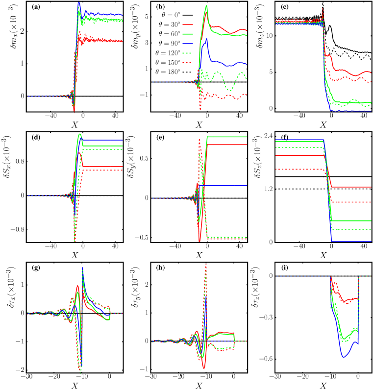
Figure 2: (Color online) In this figure, we present spin transport quantities as functions of position, $k_{F}x\equiv X$, for several relative angles, $\theta$, between the exchange fields in the $F_{1}$ and $F_{2}$ layers of half-metallic $F_{1}F_{2}S$ tunneling junctions. The external bias is set to be twice of the bulk superconducting pair amplitude, $V=2\Delta_{0}$. The thicknesses of ${F_{1}}$, ${F_{2}}$, and $S$ are set to be $300/k_{F}$, $10/k_{F}$, and $130/k_{F}$, respectively. Panels (a)-(c) in the first row show the dynamical part, $\delta{\bm{m}}$, of the three magnetization components, computed from Eqs. (33). Panels (d)-(f) in the second row depicts each component of the dynamical part of the spin currents, $\delta{\bm{S}}$, according to Eqs. (34). Spin currents are in general third-rank tensors in three-dimensional space. However, since our system is quasi-one-dimensional, they are reduced to three-dimensional vectors. Panels (g)-(i) in the third row presents the dynamical part of the three components of the spin-transfer torque $\delta{\bm{\tau}}$, by using the relation $\delta{\bm{\tau}}=\delta{\bm{m}}\times{\bm{h}}$. From the figure, one can easily verify the formula $\delta\tau_{i}=\partial S_{i}/\partial x$ for all $\theta$.

In Fig. 2, we present the angular dependence of the induced magnetizations, spin currents, and spin-transfer torques for the half-metallic spin valve shown in Fig. 1. The half-metallic layer $F_{1}$ is adjacent to a thinner and relatively weak ferromagnet with $h_{2}=10^{-1}E_{F}$. We begin by giving simple physical reasons for choosing these parameters. The thickness of $F_{2}$ is chosen to be thin compared to $F_{1}$ and $S$ in order to take advantage of the superconducting proximity effects. For the same reason, the exchange field in $F_{2}$ also needs to be weak enough to study the interplay between the superconducting proximity effects and spin-valve effects. In our coordinate system, $X=0$ corresponds to the interface between $F_{2}$ and $S$. Therefore, in Fig. 2, the half-metal $F_{1}$ lies in the range $X<-10$, the superconductor is in the region $X>0$, and the $F_{2}$ layer is in the region $-10<X<0$. The bias across the junction is set to be $2\Delta_{0}$ in the figure, where $\Delta_{0}$ is the singlet pair amplitude in the bulk limit. Recall that in our considerations, the exchange field in $F_{1}$ is along the $\hat{z}$ axis and in $F_{2}$ it is tilted with respect to the $\hat{z}$ axis by an angle $\theta$ in the $yz$ plane. There are two main effects that need to be taken into account in order to understand the induced magnetizations: First, the magnetic moments in $F_{1}$ and $F_{2}$ interact, with the magnetization of $F_{1}$ leaking into $F_{2}$, and vice versa, resulting in spatial precession. Secondly, both the direction and magnitude of the static magnetic moments in $F_{2}$ will affect any induced magnetizations when an external bias is present.

For the three components of the induced magnetizations (Panels (a)-(c) in Fig. 2), we first see that $\delta m_{x}$ and $\delta m_{y}$ vanish throughout the entire junction when $\theta=0^{\circ}$ and $180^{\circ}$. This is because the contributions from both the precession and static magnetizations are zero when the exchange fields are parallel ($\theta=0^{\circ}$) or anti-parallel ($\theta=180^{\circ}$) to each other. Let us first focus on $\delta m_{x}$ for other relative angles. The magnitudes for $\theta$ and $\pi-\theta$ are of the same order in the $S$ region because the $x$ component of the static magnetization is not present (recall that the exchange fields in our system are always in-plane) and only the precession effect is at work. Turning to the $\delta m_{y}$ panel, its magnitude in $S$ for $\theta=90^{\circ}$ (the exchange field in $F_{2}$ is along $y$) is determined purely from the static magnetization because the precession effect will only affect $\delta m_{x}$ and $\delta m_{z}$ at this angle. Physically, this tells us that the system becomes spin-polarized in the $xy$ plane in $S$. When $90^{\circ}<\theta<180^{\circ}$, the contribution to $\delta m_{y}$ from the precession effect is negative while the contribution from the effect of the static magnetization in $F_{2}$ is positive. The cumulative result is that the magnitudes are much smaller than their counterparts for $0^{\circ}<\theta<90^{\circ}$ in the $S$ region. For $\delta m_{z}$, we can see that it is the only non-zero component throughout the junction for parallel ($\theta=0^{\circ}$) and anti-parallel ($\theta=180^{\circ}$) configurations. The behaviors for other relative angles are simply explained again by the precession effect, just as in the case for $\delta m_{x}$.

Next, we analyze the behaviors of the induced spin currents and spin transfer torques. The spin-transfer torques are determined by the expression, Eq. (31), which are in turn related to the spin currents given in Eqs. (32) and (34). This is clearly seen in the steady state, where their interplay is encapsulated by the expression, $\frac{\partial\bm{S}}{\partial y}=\tau$. More generally, one can intuitively understand the role of the induced spin currents $\delta{\bm{S}}$ by considering the static magnetizations in each of the ferromagnetic layers. The $F_{1}$ layer is relatively thick, and can be regarded as a spin source, which polarizes the incoming current along the $+z$ direction. When a spin current originating from $F_{1}$ flows into $F_{2}$, the polarization state can be rotated by means of the local exchange field in $F_{2}$ and corresponding induced STT. For the $z$ component of the induced spin currents, $\delta S_{z}$, at $\theta=0^{\circ}$, it is constant throughout the entire junction including the superconducting layer as the spin density along $z$ commutes with the Hamiltonian. The same argument holds for the other collinear orientation $\theta=180^{\circ}$. However, the magnitude of $\delta S_{z}$ is larger at $\theta=0^{\circ}$ than at $\theta=180^{\circ}$, as a consequence of the exchange fields in the $F_{1}$ and $F_{2}$ layers being oppositely directed while $h_{1}\gg h_{2}$. In fact, the magnitude of $\delta S_{z}$ is higher when $\theta<90^{\circ}$ than the counterparts at $\pi-\theta$, for exactly the same reasons. Although $\delta S_{z}$ at $\theta=90^{\circ}$ vanishes inside the superconductor, we found that in general, this is not necessarily the case. The magnitude and the sign of $\delta S_{z}$ depend on both the thickness of $F_{2}$ and the strength of the exchange field. Thus, by carefully choosing the thickness of the second ferromagnet, which plays an important role in both triplet proximity effects and spin-transfer torques, in principle the spin transport properties of spintronics devices can be manipulated experimentally.

Let us now turn our attention to the remaining components, $\delta S_{x}$ and $\delta S_{y}$. In the collinear configurations ($\theta=0^{\circ}$ and $\theta=180^{\circ}$), both the $x$ and $y$ components are zero because of the absence of the precession effect. Both the sign and magnitude of $\delta S_{y}$ in the $S$ region roughly follow the $y$ component of the exchange field in $F_{2}$. Although the $y$ component of the exchange field in $F_{2}$ is at its maximum when $\theta=90^{\circ}$, we find that the corresponding $\delta S_{y}$ in $S$ is smaller than when at the other angles. This is because when $\theta\neq 90^{\circ}$, the $y$ component of the spin density can still be induced via the spin density precession coming from the half-metallic layer that possesses a much larger magnetization strength, which in turn is more dominant than the other effect. For the same reason, $\delta S_{y}$ in $S$ is higher at $\theta$ than at $\pi-\theta$, where $\theta<90^{\circ}$. The precession effect is seen to play an important role as well in the behavior of $\delta S_{x}$, where as panel (d) shows, at $\theta=90^{\circ}$, the dynamical part $\delta S_{x}$ abruptly increases in $F_{2}$, and then uniformly extends into the $S$ region where it is maximized.

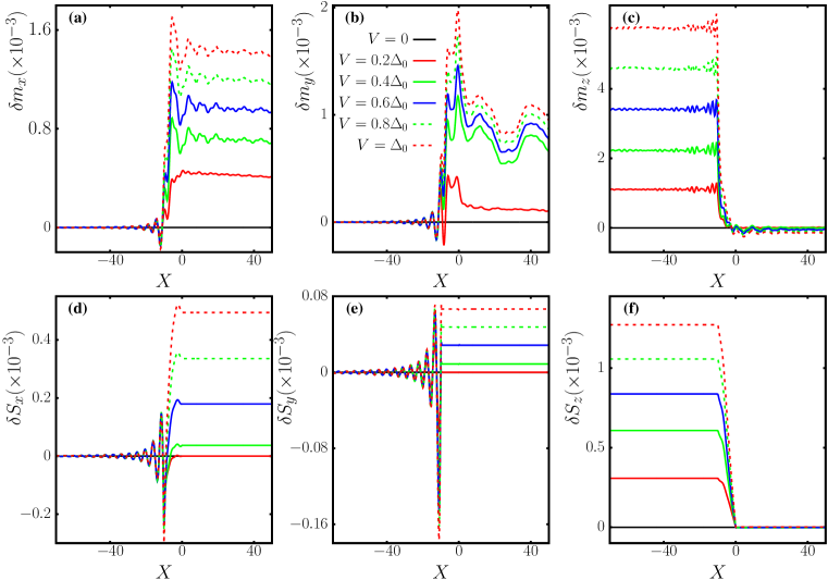
Figure 3: (Color online) In this figure, we present spin transport quantities as functions of position, $k_{F}x\equiv X$, for several external biases, $V$, scaled by the bulk superconducting gap, $\Delta_{0}$, in half-metallic $F_{1}F_{2}S$ tunneling junctions. The relative angle $\theta$ between exchange fields in $F_{1}$ and $F_{2}$ is set to be $90^{\circ}$. The thicknesses of $F_{1}$, $F_{2}$, and $S$ are set to be $300/k_{F}$, $10/k_{F}$, and $130/k_{F}$, respectively. Panels (a)-(c) in the first row show the dynamical part, $\delta{\bm{m}}(V)$, of the three magnetization components, computed from Eqs. (33). Panels (d)-(f) in the second row show the dynamical part, $\delta{\bm{S}}(V)$, of the three spin current components, computed from Eqs. (34).

The last interesting quantity is the spin-transfer torque, which is numerically determined using the relations involving the self-consistently calculated $\delta\bm{m}$ and the exchange field $\bm{h}$ [see Eq. (31)]. Since $\bm{h}$ vanishes identically inside the superconductor, all components of $\delta\bm{\tau}$ must vanish there. The absence of a torque in the superconductor imposes that the spin current there cannot vary in space as Eq. (29) shows. Thus the constancy of the spin currents inside the superconducting region shown in Fig. 2. It is also straightforward to understand why $\delta\tau_{z}=0$ in the half-metal $F_{1}$. We find that $\delta\tau_{z}$ is maximized in $F_{2}$ when $\theta=90^{\circ}$, suggesting that the corresponding $\delta S_{z}$ must have the greatest change in $F_{2}$. Indeed, as can be seen in panel (f), the only spatially varying region is in the ferromagnet $F_{2}$, and it occurs the greatest when $\theta=90^{\circ}$. We emphasize here that the static part of $\tau_{x}$ is in general non-vanishing as long as the in-plane exchange fields are non-collinear in the ${F_{1}F_{2}S}$ tunneling junctions. The static part of $\tau_{x}$ is much larger than the dynamic part. Therefore, the behavior $S_{x}$ does not significantly change with the presence of bias (not shown). In panel (e), it was observed that the precessional effect combined with the magnetization rotation in $F_{2}$, led to a reversal in the bias-induced spin current variation as $\theta$ changed. These abrupt changes in $\delta S_{x}$ translate into torque reversals within the relatively weaker ferromagnet region, as well as drastic variations near the $F_{1}$/$F_{2}$ interface, as demonstrated in (h).

In the linear-response regime, transport quantities are in principle dependent on the external bias, $V$. However, with the presence of superconductors, transport quantities sometimes exhibit distinct behavior above and below the superconducting gap. The related transport phenomena including excess current and tunneling conductance are thoroughly discussed in Refs. wvh14, ; btk, . This gap-dependent feature can be attributed to Andreev reflections. When the external bias is below the superconducting gap, current is not suppressed due to the mechanism of the Andreev scattering. Once the external bias is above the gap, the contribution to current from ordinary scattering emerges. As explained in Sec. II, the superconducting pair amplitudes are determined self-consistently and the gap profiles are position-dependent, which saturate deep inside the bulk superconductor. The saturation values of the gap profiles are important and usually smaller than the bulk superconducting gap, $\Delta_{0}$. Furthermore, the saturation values also depend on the relative magnetization angle, $\theta$.

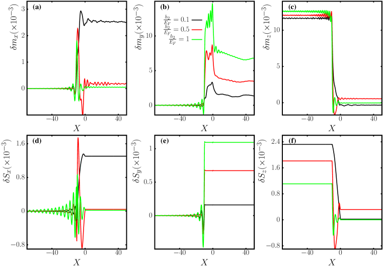
Figure 4: (Color online) In this figure, we present spin transport quantities as functions of position, $k_{F}x\equiv X$, for three different $h_{2}$ measured in terms of the Fermi energy for half-metallic $F_{1}F_{2}S$ tunneling junctions. The external bias is fixed to be twice the bulk superconducting gap, $V=2\Delta_{0}$. The relative angle $\theta$ between exchange fields in $F_{1}$ and $F_{2}$ is also fixed and its value is $90^{\circ}$. The thicknesses of ${F_{1}}$, ${F_{2}}$, and $S$ are set to be $300/k_{F}$, $10/k_{F}$, and $130/k_{F}$, respectively. Panels (a)-(c) in the first row show the dynamical part, $\delta{\bm{m}}(V=2\Delta_{0})$, of the three magnetization components, computed from Eqs. (33). Panels (d)-(f) in the second row show the dynamical part, $\delta{\bm{S}}(V=2\Delta_{0})$, of the three spin current components, computed from Eqs. (34).

In Fig. 3, we plot spin transport quantities at several different biases for $\theta=90^{\circ}$. The thicknesses of each layer and exchange interactions are the same as in Fig. 2. Our self-consistent calculations reveal that the saturation value for the superconducting gap is approximately $0.3\Delta_{0}$. First, we note the trivial fact that the dynamic part of all spin transport quantities vanishes when $V=0$. We then pay particular attention to the behavior above and below the saturation point $0.3\Delta_{0}$. Note that all three components of $\delta\bm{m}$ do not significantly change qualitatively with increased bias, and the major quantitative change is their magnitudes. Nevertheless, $\delta m_{y}(V=0.2\Delta_{0})$ is greatly suppressed compared to $\delta m_{y}(V>0.2\Delta_{0})$ while $\delta m_{x}(V=0.2\Delta_{0})$ is not. We also see that the magnitudes of both $\delta m_{x}$ and $\delta m_{y}$ increase linearly with $V$ for $V>0.3\Delta_{0}$. On the other hand, $\delta m_{z}$ does not show very distinct behavior above or below $0.3\Delta_{0}$, and it increases linearly in the entire $V$ range we considered here.

For the dynamic part of the spin currents $\delta{\bm{S}}$, we find that $\delta S_{x}$ and $\delta S_{y}$ disappear inside the superconducting region when $V<0.3\Delta_{0}$. This is due to the fact that any spin polarized current entering the superconductor is converted into a supercurrent, which is spin unpolarized. For $V>0.3\Delta_{0}$, the magnitudes inside the superconductor increase linearly with the bias, similar to what was found for $\delta m_{x}$ and $\delta m_{y}$. At these larger bias voltages, $\delta S_{x}$ and $\delta S_{y}$ within the half-metal are insensitive to changes in $V$. Examining panel (f), the current entering the $F_{1}$ region becomes strongly polarized by the half-metal, and $\delta S_{z}$ increases nearly linearly with greater bias before decaying away after interacting with the adjacent ferromagnet whose exchange field is orthogonal to it (along $y$). It is evident that unlike $\delta S_{x}$, there are no abrupt changes in behavior about the saturation point $0.3\Delta_{0}$. Examining the top row of Fig. 3, one can infer the qualitative behavior of the torque throughout the structure. Thus, the bias dependence to the spin transfer torque is omitted here, as it clearly follows that of $\delta{\bm{m}}$.

Next, we explore spin transport properties with different strengths of the exchange field in $F_{2}$ while fixing the exchange field in $F_{1}$ to be $h_{1}=E_{F}$. In Fig. 4, we plot $\delta{\bm{m}}$ (top row) and $\delta{\bm{S}}$ (bottom row) for three different $h_{2}$. The relative angle between the exchange fields in $F_{1}$ and $F_{2}$ is again fixed at $\theta=90^{\circ}$ (the direction of the exchange interaction in $F_{2}$ is along $y$), and the bias is set at $V=2\Delta_{0}$. In panel (b), we see that the overall trends in the induced magnetization do not change significantly for different $h_{2}$, where $\delta m_{y}$ is damped out in the half-metal, and then peaks in $F_{2}$ before propagating into the superconductor. The half-metal has its exchange field aligned in the $z$ direction, thus the current is initially polarized in this direction leading to a nearly vanishing $y$ component of the induced magnetization, which becomes $y$ polarized when entering adjacent ferromagnet. The result is that $\delta m_{y}$ from both $F_{1}$ (due to the precession effect) and $F_{2}$ (due to the inherent magnetization) extend into the superconductor with a magnitude proportional to $h_{2}$. For the induced magnetization normal to the interfaces, $\delta m_{x}$, we see that it builds up within $F_{2}$, and then undergoes damped oscillations (see panel (a)). The period of these oscillations in $F_{2}$ are governed by the degree of spin polarization in the ferromagnet and thus scale inversely proportional to $h_{2}$. Therefore, one can see that for such a thin $F_{2}$, $\delta m_{x}$ with $h_{2}=0.1$ is too confined to possess even a full period of oscillation. As a result, when $h_{2}=0.1E_{F}$, $\delta m_{x}$ becomes “squeezed” and has a larger magnitude in $F_{2}$ compared to when $h_{2}=0.5E_{F}$ and $h_{2}=E_{F}$. If we increase the thickness of $F_{2}$, $\delta m_{x}$ for $h_{2}=0.1E_{F}$ will also become negligible inside the $S$ layer. This property provides a way for experimentalists to control the flow of magnetization by varying the thickness of the intermediate ferromagnetic layer. Turning now to panel (c), it is seen that inside $F_{1}$, $\delta m_{z}$ is only very weakly dependent on $h_{2}$ and is uniform in space. Inside $F_{2}$ it exhibits damped oscillations, akin to $\delta m_{x}$, with an oscillation period that is inversely proportional to $h_{2}$. If the $F_{2}$ layer is thick enough, $\delta m_{z}$ will vanish identically inside the $S$ layer, irrespective of $h_{2}$. This sensitivity to thickness can be used to control not only whether $\delta m_{z}$ vanishes in the $S$ layer, but also for appropriate thicknesses, whether it can be positive or negative.

Now, let us compare spin currents for different $h_{2}$. From panel (e), we see that for a given $h_{2}$, the induced $\delta S_{y}$ is constant and flows uninterrupted inside both the $F_{2}$ and $S$ layers. This is a reflection of the fact that the $y$ component of the spin-transfer torque vanishes in those regions. As Eq. (31) showed, this can also be found by simply computing the cross product between $\delta\bm{m}$ and $\bm{h}$. For the same reasons, $\delta S_{x}$ is constant inside the $S$ layers only, while $\delta S_{z}$ is constant in the $F_{1}$ and $S$ regions. For each $h_{2}$, the relative magnitudes of $\delta\bm{S}$ in $F_{2}$ and the superconducting region follow similar trends as $\delta\bm{m}$, in that there is a positive correlation between the corresponding components of $\delta\bm{S}$ and $\delta\bm{m}$. We also find that the spatial period for the oscillation inside the $F_{2}$ layer is the same as that of $\delta\bm{m}$ for a given $h_{2}$. Finally, it is important to stress that both the direction and the magnitude of $\delta\bm{S}$ can also be adjusted by changing the $F_{2}$ thickness. In practice, one would like to choose a weaker ferromagnet for this intermediate layer. This follows not only from the potential triplet pair enhancement (discussed below), but also when a strong ferromagnet is adopted, the $F_{2}$ thickness should be relatively thin in order to take advantage of this thickness sensitivity. As before, we do not present the spin-transfer torques here since they can be computed directly from knowledge of $\delta\bm{m}$ [Fig. 4, first row], and $\bm{h}$.

We now focus on the induced triplet correlations for these half-metallic tunneling $F_{1}F_{2}S$ junctions. It is useful to recall that the triplet correlations can be induced even in the absence of an external bias wvh12 . As discussed in Ref. wvh12, , triplet correlations with $m=\pm 1$ projections on the spin quantization axis are important since these spin-polarized pairs are immune to pair-breaking effects of the exchange fields in the $F$ layers. This is especially relevant when a very strong half-metallic layer is present. Successful control of a dissipationless supercurrent is regarded as one of the essential goals in the development of practical low-temperature spintronics devices. Presumably, this can be achieved by generating and controlling the $f_{1}$ and $f_{2}$ equal-spin triplet pairs, hvw15 since they are able to propagate over relatively long distances without serious degradation. To simplify the discussions below, we shall focus on the $f_{1}$ equal-spin and $f_{0}$ opposite-spin triplet channels, since in many cases $f_{2}$ behaves complimentary to $f_{1}$.

The physics of induced triplet correlations for spin valves in the static limit has been extensively discussed in Ref. wvh12, . Also, we find that in the $F_{1}$ layer the dynamic part is added constructively to the static part of the triplet amplitudes. Therefore, we focus here on the dynamical situation where the external bias is non-vanishing and confine our attention to the dynamic part of the induced triplet correlations. To find the bias dependence to the triplet pairs in our system, we define, similar to previous quantities, the induced triplet correlations via $\delta f_{i}(V)=f_{i}(V)-f_{i}(V=0)$, where $i=0,1$.

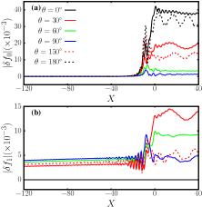
Figure 5: (Color online) The dynamical part of the induced triplet correlations as functions of position, $X$, for several angles $\theta$. In panel (a) we have $\delta f_{0}(V=2\Delta_{0})$ [see Eq. (25a)], and in panel (b) we have $\delta f_{1}(V=2\Delta_{0})$ [see Eq. (25b)]. The external bias is fixed to be twice that of the bulk superconducting gap, $V=2\Delta_{0}$. The relative time of these triplet correlation is $\omega_{D}t=4$. The thicknesses of $F_{1}$, $F_{2}$, and $S$ are set to be $300/k_{F}$, $10/k_{F}$, and $130/k_{F}$, respectively. The exchange fields are $h_{1}=E_{F}$ and $h_{2}=0.1E_{F}$.

In Fig. 5, we present the angular dependence of both the opposite-spin $f_{0}$ and equal-spin $f_{1}$ triplet pairs. The pair correlations are functions of their relative time difference $t$, which is set according to the dimensionless relation $\omega_{D}t=4.0$. The external bias is fixed at $V=2.0\Delta_{0}$. The thicknesses are the same as in previous figures, with the exchange fields in $F_{1}$ and $F_{2}$ again corresponding to $h_{1}/E_{F}=1$ and $h_{2}/E_{F}=0.1$, respectively. For $\delta f_{0}$ shown in the top panel (a), we find that it decays into the half-metallic layer with a very short decay length, as it is energetically unstable due to the presence of a single spin band at the Fermi level. Within the thin ferromagnet ($-10<X<0$), $\delta f_{0}$ is largest when a single quantization axis can be ascribed to the system, i.e., when the magnetizations of both $F$ layers are collinear. There is a slightly more pronounced effect when $\theta$ corresponds to the antiparallel configuration, where there are greater competing effects between the magnetizations in the $F_{1}$ and $F_{2}$ layers. When $F_{1}$ and $F_{2}$ are in the orthogonal configuration with $\theta=90^{\circ}$, they are then in their most inhomogenous magnetic state, and the $\delta f_{0}$ amplitude is lowest in $F_{2}$. For other orientations that are closest to the orthogonal configurations, such as $\theta=60^{\circ}$, $\delta f_{0}$ is also relatively weak compared to the collinear situation, but larger compared to $\theta=90^{\circ}$ due a finite $z$ component to the magnetization. These findings for the thin ferromagnet layer carry over to the superconducting layer, where the following angular dependence is observed: $\delta f_{0}$ is minimized at $\theta=90^{\circ}$ (orthogonal configuration) and maximized for the collinear configurations ($\theta=0^{\circ}$ and $180^{\circ}$).

We turn now to the more interesting $\delta f_{1}$ component, which is much more robust against the magnetic pair-breaking effects. In the bottom panel (b), we present the spatial behavior of $\delta f_{1}$, again for several $\theta$. We first see that $\delta f_{1}$ vanishes for the collinear configuration, as it should, as explained earlier in the introduction. For other relative angles, $\delta f_{1}$ is generated because of the non-collinear magnetic profile which prevents the system from being described by a single quantization axis. Furthermore, as shown in panel (b), the bias-induced $\delta f_{1}$ triplet amplitude is long-ranged in the half-metal and maximized for orientations around $\theta=90^{\circ}$. This is the central result of this subsection. Once the spin-polarized triplet pairs pass through $F_{2}$, they enter the superconductor and become enhanced, not for the orthogonal configuration, but rather for slight misalignments in the relative magnetizations. These trends are similar to what was observed in Fig. 2 for the $y$-component of the bias induced magnetization. Thus, we have demonstrated the long-range nature of the dynamic part of the triplet pairs by showing that only the $\delta f_{1}$ component survives in the half-metal. Also, due to the interactions between $F$ layers and triplet conversion effects, spin-polarized triplets were shown to be effectively generated within the $S$ region. Moreover, our study revealed that $\delta f_{0}$ in $F_{2}$ and $S$, and $\delta f_{1}$ in the half-metal are often anticorrelated, i.e.,when $\delta f_{0}$ is maximized (minimized), $\delta f_{1}$ is minimized (maximized).

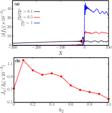
Figure 6: (Color online) In panel (a) of this figure, we present the dynamical part of induced triplet correlations, $\delta f_{1}$, as functions of position, $X$, for three different normalized exchange fields in the $F_{2}$ layer: $h_{2}/E_{F}=0.1$, $h_{2}/E_{F}=0.5$, and $h_{2}/E_{F}=1.0$. The angle $\theta$ between exchange fields in $F_{1}$ and $F_{2}$ is chosen to be $\theta=90^{\circ}$. The external bias is fixed at twice the bulk gap, $V=2\Delta_{0}$. The thicknesses of $F_{1}$, $F_{2}$, and $S$ are set at $300/k_{F}$, $10/k_{F}$, and $130/k_{F}$, respectively. In panel (b), we show the normalized charge current density v.s. the exchange field $h_{2}$ of the intermediate $F$ layer. The data points are connected by lines to serve as guides to the eye. The relative angle between the exchange fields in $F_{1}$ and $F_{2}$ is $90^{\circ}$.

It was mentioned at the beginning of this subsection that our choice of $h_{2}/E_{F}=0.1$ for the exchange field strength in the thin intermediate $F_{2}$ layer, resulted in the optimal amount of spin-polarized pairs in the half-metallic region. To illustrate this, it is insightful to consider differing exchange field magnitudes in $F_{2}$ and examine how these differences affect the equal-spin triplet pairs throughout the entire junction. Thus, we present in panel (a) of Fig. 6, the spatial dependence of the magnitude of the dynamic part $\delta f_{1}$ for several $h_{2}$. We set $\theta=90^{\circ}$, creating the most magnetically inhomogenous configuration possible, and thus maximizing $\delta f_{1}$ in $F_{1}$. Note that here the spatial range is much wider than the results presented before in order to identify any long range behavior of the spin-polarized triplet correlations. First, inside the superconducting layer, we find that the magnitude of $\delta f_{1}$ is approximately proportional to $h_{2}$. However, in the non-superconducting regions, $\delta f_{1}$ for both $h_{2}/E_{F}=0.5$ and $h_{2}/E_{F}=1.0$ decays with a very small characteristic decay length. On the other hand, the weaker exchange field of $h_{2}/E_{F}=0.1$ results in $\delta f_{1}$ penetrating quite extensively into the $F$ regions, thereby establishing its long range behavior. This result is significant, and it justifies our choice of for $h_{2}$, mentioned earlier. Although we do not show the static part of the induced triplet correlations, we find the same behavior as before: the static part of $f_{1}$ is long-ranged when the magnetic configuration is non-collinear and its magnitude is comparable to the dynamic part. In the absence of a bias voltage, the corresponding static $f_{1}$ amplitudes are also maximized when $h_{2}\sim 0.1E_{F}$.

To further corroborate these ideas, we show in panel (b) of Fig. 6 the charge current density, $J_{x}$, along the direction perpendicular to the interface as a function of $h_{2}$. The current density is normalized by $J_{0}\equiv en_{e}v_{F}$, where $n_{e}$ is the electron density and $v_{F}\equiv k_{F}/m$ is the Fermi velocity. Here we fix the external bias to be $V=2.0\Delta_{0}$ and the relative angle between the exchange fields in the $F_{1}$ and $F_{2}$ layers is $\theta=90^{\circ}$. As in Refs. hvw15, and wvh14, , it is stressed that the current density is spatially uniform throughout the junction in order to satisfy the continuity equation. In the $S$ region one should consider both the current density computed from Eq. (19) and also the integration of the source term in Eq. (16), since the pair potential is not zero there. To avoid this complexity, we compute the current density from Eq. (19) directly in the $F$ region. Furthermore, we verify that if one includes the contribution from the source term, the current density is indeed uniform across the entire tunneling junctions. From panel (b) of Fig. 6, we find that the current density is maximized at $h_{2}/E_{F}=0.1$. Recalling that the equal-spin triplet correlations $f_{1}$ are the most long-ranged at $h_{2}/E_{F}=0.1$, this suggests a correlation between the long-ranged nature of the spin-polarized triplet pairs and the charge transport. Finally, we see that the charge density is lowest at $h_{2}/E_{F}=1$, where only one spin band is accessible in both $F$ layers for the current carrying states. The results presented in Fig. 6 therefore strongly suggest that by using relatively thin ferromagnets with weak exchange fields, the half-metallic region will effectively host long-range spin-polarized triplet pairs that offer hints of their signatures in the charge transport behavior. Thus, to achieve these properties for the structures considered here, $h_{2}/E_{F}=0.1$ is the optimal strength for such half-metallic superconducting spintronic devices. If on the other hand it is desired to generate $f_{1}$ triplet pairs solely in the superconductor, one should incorporate half-metals into both $F$ regions.

III.2 Half Metallic Josephson Junctions

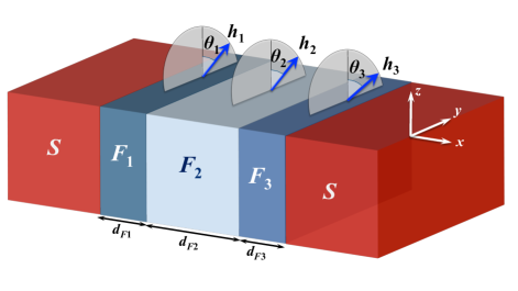
Figure 7: (Color online) Schematic of the $SF_{1}F_{2}F_{3}S$ Josephson junction. The layers are translationally invariant and extend to infinity in the $yz$ plane. The central $F_{2}$ layer is half-metallic ($h_{2}=E_{F}$), while the surrounding $F_{1}$ and $F_{3}$ layers are ferromagnets with weaker exchange fields $h_{1}=h_{3}=0.1E_{F}$. The angles $\theta_{1}$, $\theta_{2}$, and $\theta_{3}$ describe the angles that the magnetic exchange field vector makes with the $z$ axis in the corresponding $F_{1}$, $F_{2}$ and $F_{3}$ layers with thicknesses $d_{F1}$, $d_{F2}$, and $d_{F3}$, respectively.

In this subsection we present our results for half-metallic $SF_{1}F_{2}F_{3}S$ Josephson junctions. A diagram of the setup is shown in Fig. 7. A trilayer magnetic configuration is considered to allow for the generation of singlet and triplet correlations by using relatively weak and thin magnets nearest the $S$ layers. For the half-metal thicknesses considered here, using a simpler bilayer structure consisting of a thick half-metal and ferromagnet would result in the destruction of phase coherence between the $S$ banks. Thus two relatively weak ferromagnets are needed to be in contact with the superconductors to effectively generate triplet correlations and establish both charge and spin currents within the junction. The thicknesses of the $S$ layers are $800/k_{F}$, while $F_{1}$, $F_{2}$, and $F_{3}$ can vary, depending on the quantity being studied. As before, the superconducting coherence length is fixed to be $100/k_{F}$. For most cases, the interfaces are generally assumed to be transparent, although cases with interface scattering will be considered as well. Unless otherwise noted, the central $F$ layer is half-metallic, with exchange field corresponding to $h_{2}=E_{F}$. Similar to what was shown for tunnel junctions, the spin-valve effect is maximized when the exchange fields of $F_{1}$ and $F_{3}$ are weaker: We consider here $h_{1}=h_{3}=0.1E_{F}$. For these Josephson structures, the focus of the investigation is on the influence that the macroscopic phase difference $\Delta\varphi$, and the relative magnetization orientations have on the spin currents, charge currents, and associated triplet correlations. To be consistent with the previous results on tunnel junctions, the magnetization is normalized by $-\mu_{B}n_{e}$, where $n_{e}$ is the electron density and the charge currents are normalized by $J_{0}$, where $J_{0}=en_{e}v_{F}$, and $v_{F}=k_{F}/m$ is the Fermi velocity. All three components of the spin current $\bm{S}$ are normalized similarly hvw15 .

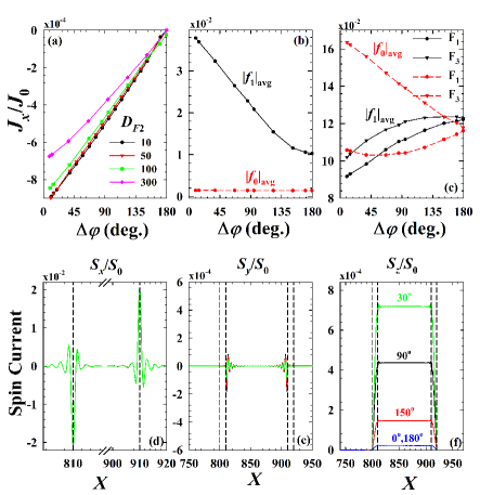
Figure 8: (Color online) First row (a)-(c): The normalized current density $J_{x}$ v.s. the phase difference $\Delta\varphi$ for (a) several normalized half-metal thicknesses $D_{F2}=k_{F}d_{F2}$. (b) The equal-spin $f_{0}$ and opposite-spin $f_{1}$ triplet correlations spatially averaged over the half metal region $F_{2}$, and (c) over the ferromagnetic $F_{1}$ and $F_{3}$ regions. Second row (d)-(f): The components of the normalized spin current $\bm{S}$ as a function of dimensionless position $X=k_{F}x$. In (a)-(f), the exchange fields in $F_{1}$ and $F_{3}$ are aligned along the $y$ direction, and along $z$ in the half-metal $F_{2}$ (see Fig. 7). The ferromagnets $F_{1}$ and $F_{2}$ have equal thicknesses of $10/k_{F}$. In panels (b)-(f) the $F_{2}$ thickness is fixed at $100/k_{F}$.

We begin with the self-consistent current phase relation for the $SF_{1}F_{2}F_{3}S$ structure shown in Fig. 7. In Fig. 8(a), the normalized charge current flowing in the $x$ direction, $J_{x}$, is shown as a function of the macroscopic phase difference $\Delta\varphi$. The central half-metallic $F_{2}$ layer is sandwiched between two weaker ferromagnets with normalized exchange field strengths $h/E_{F}=0.1$, and thicknesses $10/k_{F}$. Each of the ferromagnets $F_{1}$ and $F_{3}$ have their magnetizations oriented in the same direction (along $y$) but orthogonal to $F_{2}$ (along $z$). To isolate the triplet spin current flowing through the half-metal, differing dimensionless thicknesses $D_{F2}=k_{F}d_{F2}$ are considered, as shown in the legend. As seen, the supercurrent essentially obeys a linear trend with phase difference that is weakly dependent on the thickness of the half-metal. As this thickness increases, the current begins to deviate from the linear behavior, as seen developing for the $D_{F2}=300$ case. The fact that increasing the thickness $D_{F2}$ has a weak effect on the supercurrent reflects the spin-polarized nature of the triplet pairs involved in transport through the half-metal. We limit the range of the current phase relation for clarity, however extending the range of $\Delta\varphi$ would result in a sawtooth-like profile with vanishing current at $\Delta\varphi=n\pi$, where is $n$ is an integer. Physically, the slow decay of the equal-spin triplet correlations in the half metal equates to propagation lengths of the quasiparticles that can well exceed $\xi_{F}$. To demonstrate this, in (b) the magnitudes of the opposite spin correlations $f_{0}$ and equal spin correlations $f_{1}$ averaged over the half-metallic region $F_{2}$ are shown. To satisfy the Pauli principle, these spatially symmetric triplet pairing correlations must be odd in time, and hence vanish when the relative time $t$ is zero. For the results involving triplet pairs in this section, we take the corresponding dimensionless time to be $\omega_{D}t=4$. Due to the presence of only one spin band in $F_{2}$, the $f_{0}$ correlations have a very weak extent within the half-metal and remain relatively constant for all $\Delta\varphi$. On the other hand, the $f_{1}$ component has a relatively large presence in $F_{2}$, increasing as the magnitude of the current increases. In the absence of current, the triplet amplitudes populate the half-metal, consistent with what is found in half-metallic spin valves half . As mentioned earlier, the presence of the thin ferromagnet layers is important for the generation of the opposite-spin triplet pairs, and consequently the conversion to the equal-spin channel. This effect is clearly seen in (c), where now the magnitude of the triplet correlations are presented averaged over the $F_{1}$ and $F_{3}$ layers. As the macroscopic phase difference changes, it is evident that a nontrivial intermixture of $f_{0}$ and $f_{1}$ occurs in those layers.

In the bottom row of panels ((d)-(f)), the three components of the normalized spin currents are shown as a function of the dimensionless position $X=k_{F}x$. All components of the spin current flow in the $x$ direction. The dashed vertical lines serve to identify the narrow ferromagnetic regions containing $F_{1}$ and $F_{3}$. If the $F$ layers possessed uniform magnetization, there would be no net spin current. The introduction of an inhomogeneous magnetization however results in a net spin current imbalance that is finite even in the absence of a Josephson current. In (d), we present the normalized $x$ component of the spin-current, $S_{x}$, which is responsible for the torque that tends to align the magnetizations in the ferromagnetic layers. This exchange field mediated effect is present in the absence of Josephson current and is seen to be almost independent of the phase difference that drives the Josephson current. As seen, this quantity is maximized at the interfaces, before undergoing damped oscillations. For completeness, we have included in (e) the $y$ component of the spin current, which for our magnetic configuration is clearly negligible. In panel (f), we examine the normalized $z$-component of the spin current $S_{z}$. This component, which is oriented parallel to the interfaces tends to build up on the weakly ferromagnetic layers and then propagate uniformly in the half-metal. The magnitude of $S_{z}$ is seen to correlate with the magnitude of the charge current in (a), where the smaller phase differences result in large charge and spin currents that decline as $\Delta\varphi$ increases. These results indicate that the half-metal polarizes the spin current along its magnetization direction, and that the Josephson current is due to the propagation of equal-spin triplet pairs.

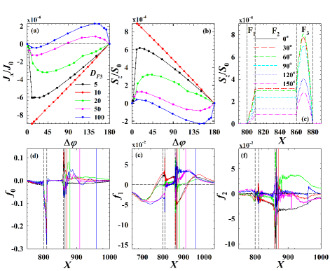
Figure 9: (Color online) Top row: (a) The normalized charge current density $J_{x}$ v.s. the phase difference $\Delta\varphi$, (b) the $z$ component of the normalized spin current density $S_{z}$ within the half-metal region v.s. $\Delta\varphi$ for several $D_{F3}$, and (c) the normalized $S_{z}$ as a function of dimensionless position $X\equiv k_{F}x$ for $D_{F3}=20$. The legend in (c) labels the different phase differences $\Delta\varphi$ (in degrees) between the $S$ banks. The legend in (a) depicts the ferromagnet thicknesses $D_{F3}$ used in (a), (b), and (d)-(f). Bottom row: The spatial behavior of the real part of the triplet correlations for various thicknesses (see legend in (a)) and for a phase difference of $\Delta\varphi=90^{\circ}$. The dashed vertical lines identify the $F_{1}$ and $F_{2}$ regions located within $800\leq X\leq 810$ and $810<X\leq 860$ respectively, while the solid vertical lines mark the various $F_{3}/S$ interfaces. The exchange field in $F_{1}$ and $F_{3}$ is aligned along the $y$ direction, while it points along $z$ in the half-metal (see Fig. 7). The thicknesses $d_{F1}$, and $d_{F2}$ are maintained at the constant dimensionless values of $D_{F1}=10$ and $D_{F2}=50$, respectively.

Next, in Fig. 9(a) the half metal $F_{2}$ and ferromagnet $F_{1}$ have fixed thicknesses corresponding to $D_{F2}=50$ and $D_{F1}=10$, respectively. The ferromagnet $F_{3}$ is allowed to vary, as shown in the legend. Asymmetric structures with unequal thicknesses of the ferromagnetic layers has been shown to enhance spin mixing effects that results in the generation of long-ranged spin-polarized triplet pairs zep . The linear behavior of the charge current previously shown in Fig. 8 where the two magnets $F_{1}$ and $F_{3}$ are of equal thickness is seen to transition to a sinusoidal-like structure as the difference in the thicknesses between $F_{1}$ and $F_{3}$ increases. Thus, for highly asymmetric structures, the current phase relation reveals a sign change in the charge current for phase differences between $0^{\circ}$ and $180^{\circ}$. The ferromagnet $F_{3}$ with relatively weak exchange field compared with $F_{2}$ and somewhat larger thicknesses ($D_{F3}=10$) creates ideal conditions for the creation and propagation of opposite-spin triplet pairs. The center of mass momentum of a given pair shifts in the presence of spin splitting from the exchange field, resulting in the observed damped oscillations for a given $\Delta\varphi$.

If we now calculate the $z$ component of the spin current flowing through the half-metal portion of the junction, we find that aside from a sign difference, it is nearly identical to the Josephson current as seen in Fig. 9(b). This reaffirms that the current flowing through the half-metal is comprised of Cooper pairs that are polarized in the $z$ direction by the half-metal. In general, the spin current is a non-conserved quantity, in contrast to the charge current. Thus, although $S_{z}$ is uniform throughout the half-metal, it spatially varies in the other junction regions. This is demonstrated in (c) for several phase differences $\Delta\varphi$ (see legend), where $D_{F1}=10$, $D_{F2}=50$, and $D_{F3}=20$. The spin current does not flow in the outer superconductor banks, and thus $S_{z}$ increases from zero at the $S/F_{1}$ interface ($X=800$) before reaching its uniform value in the half metal, and then peaks within $F_{3}$ before declining to zero again in the superconductor.

To reveal the relative population of triplet pairs throughout the junction, we consider in (d)-(f) the triplet correlations $f_{0}$, $f_{1}$, and $f_{2}$, as functions of normalized position $X$. The phase difference is set according to $\Delta\varphi=90^{\circ}$. We still have $D_{F1}=10$, and $D_{F2}=50$, but several $D_{F3}$ are shown with values given in the legend found in panel (a), thus creating a broad range of current profiles. The opposite-spin triplet correlations shown in (d) reveal that $f_{0}$ spikes in the $F_{1}$ region, weakly dependent on $D_{F3}$. Within $F_{2}$ however, the single spin band present in the half-metal severely diminishes $f_{0}$. When $F_{3}$ has thin layers, the greater confinement enhances the $f_{0}$ amplitudes. Increasing $D_{F3}$ eventually provides sufficient space for the exchange field to induce damped oscillations of the opposite-spin pairs. Thus, although it is energetically unfavorable for the $f_{0}$ correlations to reside in the half metal, they do become enhanced in the surrounding ferromagnets when they are thin ($D_{F3}=5,10$). Under these conditions, the spin polarized triplet pairs $f_{1}$ and $f_{2}$ propagate within the half metallic region, as seen in (e) and (f). It is also evident that often the equal-spin triplets do not decay within the $S$ regions, but rather extend deep into the superconductor banks.

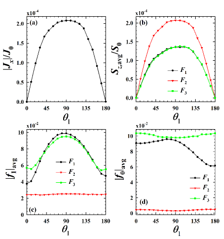
Figure 10: (Color online) Top row: (a) Normalized charge currents and (b) the $z$ component of normalized spin currents in each junction region as a function of the magnetization alignment angle $\theta_{1}$. Bottom row: Spatially averaged equal-spin (c) and opposite-spin (d) triplet correlations as a function of $\theta_{1}$.The thicknesses of ${F_{1}}$, ${F_{2}}$, and ${F_{3}}$ are set to be $10/k_{F}$, $50/k_{F}$, and $10/k_{F}$, respectively. An interface scattering strength of $H_{1,4}=0.8$ is present at the interfaces (see main text), and a phase difference of $\Delta\varphi=90^{\circ}$ is assumed.

Having seen the influence that the layer thicknesses in half-metallic Josephson junctions have on the charge and spin currents, we now turn to the the effects of magnetization rotations. Rotating the magnetization in one of the junction layers can be achieved experimentally via external magnetic fields, or spin-torque switching. In Fig. 10(a) we display the magnitude of the normalized charge current as a function of the magnetization angle $\theta_{1}$. The half metal thickness is set at $D_{F2}=50$, and the surrounding ferromagnets have equal thicknesses of $D_{F1}=D_{F3}=10$. The effects of scattering at the $S/F_{1}$ and $F_{3}/S$ interfaces are accounted for by setting the dimensionless parameter $H_{B1}\equiv H_{1}/v_{F}=0.8$ and $H_{B4}\equiv H_{4}/v_{F}=0.8$, respectively. Here $H_{1}$ and $H_{4}$ are the delta-function scattering strengths at those two interfaces hvw15 . The inclusion of interfacial scattering in Josephson junctions tends to suppress the linear sawtooth profile in the current phase relation hvw15 . The Josephson current is established with a phase difference $\Delta\varphi=90^{\circ}$ between the superconducting banks. The half metal layer has its ferromagnetic exchange field directed along $z$ and for $F_{3}$, it is directed along $y$ (see Fig. 7). Thus, when $\theta_{1}=0^{\circ}$ or $\theta_{1}=180^{\circ}$, both $F_{1}$ and the adjacent half metallic layer have magnetizations that are parallel or antiparallel, respectively. At these points, $J_{x}$ vanishes while the supercurrent flow is largest when $\theta_{1}=90^{\circ}$, corresponding to when the junction layers have magnetizations that are orthogonal to one another, and hence possess a high degree of magnetic inhomogeneity. The half-metal tends to align the spin of any entering quasiparticles along the $z$ direction, and this component of the normalized spin current displays nearly identical behavior to $J_{x}$ as seen in (b). The averaged spin current is distributed equally throughout the two outer ferromagnets, but weaker overall since it must vanish at the boundaries with the superconductors. The behavior of the magnitudes of the triplet correlations v.s. $\theta_{1}$ is presented in panels (c) and (d). When $\theta_{1}=0^{\circ}$ or $\theta_{1}=180^{\circ}$, the generation of equal-spin triplets are suppressed in the ferromagnets $F_{1}$ and $F_{3}$ due to the lowering of the overall magnetic inhomogeneity. For these situations, the magnetizations in the $F_{1}$ and $F_{2}$ layers are collinear, however, $f_{1}$ does not vanish due to the orthogonal magnetization in $F_{3}$. On the contrary, when $\theta_{1}=90^{\circ}$, the magnetization in each ferromagnet is orthogonal to the adjacent one, resulting in favorable conditions for the creation of the equal spin triplets. In (d) the importance of having relatively weak and thin outer ferromagnets for the triplet conversion process is exhibited by the population of the $f_{0}$ triplet components in those regions.

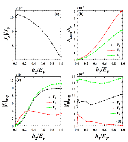
Figure 11: (Color online) Top row: Normalized charge current (a) and average spin currents (b) v.s. the dimensionless magnetization strength $h_{2}/E_{F}$. Bottom row: Spatially averaged equal-spin (c) and opposite-spin (d) triplet correlations as a function of $h_{2}/E_{F}$. The thicknesses of $F_{1}$, $F_{2}$, and $F_{3}$ are set to be $10/k_{F}$, $100/k_{F}$, and $10/k_{F}$, respectively. The legend in (b) identifies each region of the junction in which the quantities in (b)-(d) are averaged over. Here, transparent interfaces are considered and $\Delta\varphi=30^{\circ}$.

It was observed that the presence of the half-metal in the junction serves to filter out the opposite-spin triplet pairs, creating a platform in which to study spin polarized triplet correlations. It is of interest to clarify the role that the exchange field strength in the half metal region has on the charge and spin transport. The top row of Fig. 11 therefore shows the magnitude of the charge current and the averaged spin current, both normalized, as a function of the exchange field strength in the half metal, $h_{2}$. The phase difference is set to $\Delta\varphi=30^{\circ}$. For clarity, the two ferromagnets have equal thicknesses, $D_{F1}=D_{F3}=10$, and there is no interface scattering present. The larger half metal has a thickness of $D_{F2}=100$, and the exchange field varies from $h_{2}=0$ to $h_{2}=E_{F}$, which coincides with a nonmagnetic normal metal and a half-metallic phase, respectively. The junction’s magnetization profile is in an optimal inhomogenous state, with alignment angles are as follows: $\theta_{1}=90^{\circ}$, $\theta_{2}=0^{\circ}$, and $\theta_{3}=90^{\circ}$, corresponding to magnetization alignments along $y$, $z$, and $y$, respectively. Examining panel (a), it is evident that the magnitude of the charge current $J_{x}$ is maximal when the $F_{2}$ layer is weakly ferromagnetic, and is minimal when $F_{2}$ is half-metallic. The spatially averaged spin current on the other hand is anticorrelated with $J_{x}$, as it monotonically increases with larger exchange fields. Indeed, $S_{z}$ vanishes when the central $F_{2}$ layer is a nonmagnetic normal metal, and peaks when it is half-metallic. When the central layer is nonmagnetic $S_{z}$ vanishes since the only active magnetic layers in this case are $F_{1}$ and $F_{3}$ which have parallel magnetization directions. Examining the bottom row, the triplet correlations are also shown averaged over each of the three junction layers. In (c) the magnitude of the $f_{1}$ correlations are shown v.s. $h_{2}/E_{F}$. When $h_{2}=0$, $F_{1}$ and $F_{3}$ are the only ferromagnetic layers in the junction, and their magnetizations are oriented along $y$. Since they are collinear, spin-polarized triplet pairs cannot be generated, and hence $f_{1}=0$. Increasing $h_{2}$ and hence the degree of polarization in the $F_{2}$ layer continuously increases the amount of spin polarized triplet pairs in the ferromagnets $F_{1}$ and $F_{3}$, with $f_{1}$ largest when $F_{2}$ is half-metallic. The $f_{1}$ correlations in $F_{2}$ also become enhanced as its exchange field get larger, until $h_{2}/E_{F}\approx 0.3$. Further increases in $h_{2}$ result in a slight decline before ultimately increasing again as $F_{2}$ approaches the half-metallic limit. This demonstrates the importance of using a highly spin-polarized material in the central junction region to optimize triplet pair generation in each layer. The opposite-spin pairs $f_{0}$ are also maximized in the triplet conversion layers $F_{1}$ and $F_{3}$ when $h_{2}=E_{F}$ as seen in (d). Unlike what is found for $f_{1}$, the $f_{0}$ correlations are not constrained to vanish when $h_{2}=0$ since they can exist when the ferromagnets have collinear magnetizations. Thus the thin ferromagnetic regions have a substantial portion of $f_{0}$ pairs when $h_{2}=0$. Within the thicker $F_{2}$ layer however, $f_{0}$ is significantly reduced overall, becoming negligibly small in the nonmagnetic metal ($h_{2}=0$) and half-metallic ($h_{2}=E_{F}$) limits. It substantiates the idea that using the half-metal for $F_{2}$ enables us to focus on the interplay between the spin current and the equal spin pairs $f_{1}$ in the $F_{2}$ region.

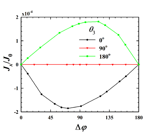
Figure 12: (Color online) Charge current as a function of phase difference $\Delta\varphi$. The thicknesses of $F_{1}$, $F_{2}$, and $F_{3}$ are set to be $10/k_{F}$, $100/k_{F}$, and $10/k_{F}$, respectively. The interface scattering strengths are set to $H_{B1}=H_{B4}=0.8$. The magnetization in $F_{1}$ and $F_{2}$ is along the $z$ and $y$ directions respectively. In the ferromagnet $F_{3}$, the magnetization orientation angles $\theta_{3}$ varies as shown ($\theta_{3}=0$ is along $z$, $\theta_{3}=90^{\circ}$ is along $y$, and $\theta_{3}=180^{\circ}$ is along -$z$).

We now take the structure previously studied above in Fig. 11 and incorporate interface scattering, and rotate the magnetizations so that they are interchanged for the first two layers. Thus, $F_{1}$ and $F_{2}$ have their magnetizations aligned along the $z$ and $y$ axes respectively. The normalized interface scattering strength is set at $H_{1}=H_{4}=0.8$. With these parameters, Fig. 12 examines the normalized Josephson supercurrent as a function of the phase difference $\Delta\varphi$. Three magnetization orientations for $F_{3}$ are investigated for each of the three panels: $\theta_{3}=0,90^{\circ}$, and $180^{\circ}$ (corresponding to the $z$, $y$, and $-z$ directions, respectively). The supercurrent reveals that, depending on whether the magnetization in $F_{3}$ is collinear or orthogonal to the adjacent half-metal, the direction of the charge current can be reversed or turned off completely. When $\theta_{3}=0$, the magnetization in each layer is orthogonal to one another, and the current phase relation reveals that when starting from zero phase difference, the magnitude of the current increases until $\Delta\varphi\approx 70^{\circ}$, before declining back to zero again at $\Delta\varphi=180^{\circ}$. Due to quasiparticle scattering that takes place at the interfaces, the coherent transport of Cooper pairs through the junction is significantly altered compared to when the interfaces were transparent, resulting in the observed overall reduction in current and deviation from the previous linear behavior found in Fig. 8. Previously, when studying how magnetization rotation affected the charge current in Fig. 10(a), we found that when two adjacent layers in the junction have collinear magnetizations, the charge current vanished. This is consistent with Fig. 12, where the current vanishes for all phase differences at $\theta_{3}=90^{\circ}$. Rotating the magnetization further to $\theta_{3}=180^{\circ}$, the magnetizations in both ferromagnets are orthogonal to the half-metal, as in the $\theta_{3}=0$ case, but antiparallel to each other. This causes a reversal of the charge current as shown.

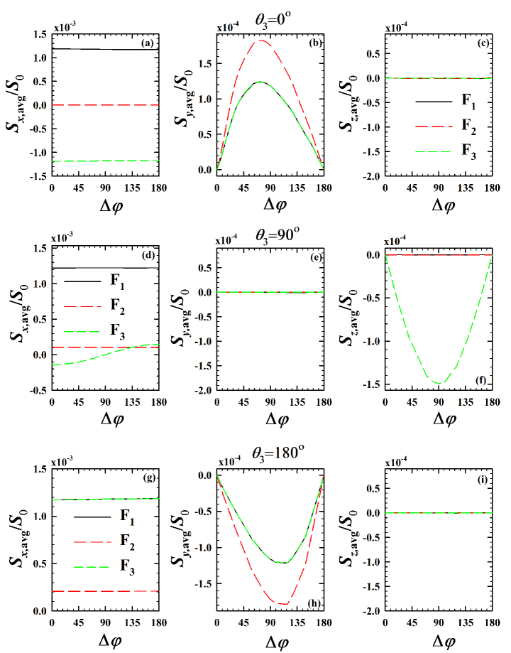
Figure 13: (Color online) Components of the average spin current in each region v.s. the phase difference $\Delta\varphi$. Three magnetization orientations of the outer ferromagnet $F_{3}$ are shown: $\theta_{3}=0$ (top row), $\theta_{3}=90^{\circ}$ (middle row), and $\theta_{3}=180^{\circ}$ (bottom row). The thicknesses of $F_{1}$, $F_{2}$, and $F_{3}$ are set to be $10/k_{F}$, $100/k_{F}$, and $10/k_{F}$, respectively. The dimensionless interface scattering strengths correspond to $H_{B1}=H_{B4}=0.8$.

As shown earlier, the charge current that flows due to the macroscopic phase differences between the $S$ electrodes can become spin-polarized when entering one of the ferromagnetic or half-metal layers. This spin current can then interact with the other ferromagnets and become modified by the corresponding magnetizations. Having established in Fig. 12 how the charge current can be manipulated for a half-metallic Josephson junction, it is important to next identify how the spin currents behave in each layer, as control of these spin currents is vital for spintronic applications. Thus, in Fig. 13 we investigate the phase dependence for the spatially averaged spin current $\bm{S}$. We implement the same experimentally accessible parameters used in Fig. 12. Each row of three panels corresponds to one of the three magnetization orientations $\theta_{3}$ (as labeled). As discussed earlier, the central half-metallic layer maintains a constant spin current, that can couple the surrounding ferromagnets $F_{1}$ and $F_{3}$. This effect is evident for $S_{x}$ when $\theta_{3}=0^{\circ}$ (top row), corresponding to the $z$,$y$,$z$ magnetic configuration for the respective $F_{1}$, $F_{2}$, and $F_{3}$ layers. This spin current component, normal to the interfaces, is essentially the static contribution to the spin current, which participates in spin-transfer torque effects near the ferromagnet/half-metal interfaces where misaligned exchange fields are present. Thus, $S_{x}$ varies in space, resulting in a local STT [recall $\partial S_{x}/\partial x=\tau_{x}$] that tends to rotate the corresponding magnetizations in opposite directions. Within the half-metal, the spin current oscillates as it damps out deep within $F_{2}$, resulting in an average $S_{x}$ of zero, as exhibited in (a). The averaged spin currents clearly do not depend on the phase difference, as expected for a static effect. The strong influence of the half-metal is exhibited by $S_{y}$, the spin current component that lies in the same direction as the exchange field in the half-metal. The half-metal is seen to polarize not only the spin current within it, but also within the surrounding weak magnets whose intrinsic exchange fields are in the orthogonal $z$ direction. Note that the $y$-component of spin currents in each of the $F$ regions have similar overall behavior as a function of $\Delta\varphi$, with the average $S_{y}$ being equal in $F_{1}$ and $F_{3}$, and largest in $F_{2}$. Comparing this to Fig. 12, it is clear that apart from a sign difference, the normalized spin current $S_{y}$ in the half-metal and the supercurrent $J_{x}$ are nearly identical. This implies that the spin-polarized current $S_{y}$ in the half-metal correlates with the charge current that is flowing there. Therefore, the charge transport is governed by spin-polarized Cooper pairs corresponding to the equal-spin correlations. Turning now to the middle row, where $\theta_{3}=90^{\circ}$, there is no spin current along $y$ for all of the $F$ layers. Within the $F_{3}$ layer, the normalized $S_{x}$ is shown to vanish at $\Delta\varphi=90^{\circ}$, while $S_{z}$ is maximal for that phase difference. Considering the phase differences that yield no supercurrent, $\Delta\varphi=0^{\circ}$ and $180^{\circ}$, The spin currents $S_{x}$ and $S_{z}$ are seen to be anti-correlated, with $S_{z}$ now vanishing, and the magnitude of $S_{x}$ having now become largest in $F_{3}$. Finally, the bottom row depicts the spin currents for $\theta_{3}=180^{\circ}$. As was found for the previous $\theta_{3}=0^{\circ}$ case, we see a direct correlation between the charge supercurrent [Fig. 12] and the $y$ component of the spin current for this magnetic configuration. The main differences being that the directions of the charge and spin currents are reversed, due to $\theta_{3}$ having a reversed collinear orientation, and non-vanishing $S_{x}$ in $F_{2}$.

IV Conclusions

In this paper, we have studied in detail the interplay between the triplet pairs and transport properties of half-metallic superconducting spin valves including tunnel junctions and Josephson junctions. In tunnel junctions with the presence of an applied bias voltage, we have discussed a useful theoretical approach combining the self-consistent solutions to the Bogoliubov-de Gennes equations and the transfer matrix method based on the Blonder-Tinkham-Klapwijk formalism. By utilizing this approach, we are able to determine the bias dependence of spin transport quantities and the induced triplet pair amplitudes. We first investigate the bias-induced magnetizations, spin currents, and the spin-transfer torques as functions of position for various misorientation angles between the half metal and adjacent weak ferromagnet. We find that their behaviors can be largely explained by the precessional effect: When the injected charge current spin-polarized by the half-metal enters the weak ferromagnet, its polarization state can be rotated by the local exchange interaction. The bias dependence of these spin transport quantities are also studied. We find that their magnitudes increase linearly when external bias voltages are larger than the saturated superconducting pair amplitudes. We then show that the spin transport quantities are determined by two important parameters: the exchange interaction and thickness of the weak ferromagnet. Both $m=0$ and $m=\pm 1$ triplet correlations of the tunnel junctions are also presented. We find that they are anti-correlated when the misorientation angle between exchange interactions in the ferromagnetic layers is varying. Furthermore, the long-range nature of $m=\pm 1$ triplet correlations in the half-metallic region is established and proven to be important in the half-metallic tunnel junctions. It is shown that choosing the exchange interaction to be about $0.1E_{F}$ can optimize the spin-valve effect. We then switch to half-metallic Josephson junctions which consist of a half metal sandwiched by two weak ferromagnets in the non-superconducting region. First, we consider a symmetric situation where the thicknesses and the exchange fields are the same for two weak magnets. To generate all components of triplet pairs, the exchange field in the half metal is perpendicular to that of weak magnets. We study the current phase relations and find that the current is only weakly dependent on the thickness of the half metal indicating that the supercurrent is carried by the equal-spin triplet pairs. This is also corroborated by the fact that the charge current is strongly correlated with the spin current as a function of the phase difference between the two superconducting banks. We also investigate the asymmetric situation where the thickness of one of the weak magnets is adjusted. We again find that the equal-spin triplet pairs are responsible for the flow of supercurrent and the spin current. Next, we analyze the effect of misorientation angle between the exchange field in the half metal and the adjacent weak magnet. When the misorientation angle is $90^{\circ}$, the charge current, the equal-spin triplet pair amplitudes, and the spin currents attain their maximum values. On the other hand, when the angle is $0^{\circ}$ or $180^{\circ}$, both the charge and spin currents vanish, showing the importance of the magnetic configuration in half-metallic Josephson junctions. The induced triplet correlations also depend on the exchange interaction for the central ferromagnet. They saturate when the half-metallic limit is reached. Finally, we show that when the exchange fields in the weak magnets have the same magnitude and are perpendicular to that of the half metal, the spin-valve effect is most pronounced.

Appendix A Spin Rotations

Here we outline the spin rotations that are performed on the triplet components ($f_{0}$, $f_{1}$, $f_{2}$) in Eq. (23). By aligning the spin axes with the local exchange field directions, the role of the triplet correlations and their physical interpretation becomes clearer. The central quantity that we use to perform the desired rotations is the spin transformation matrix $\mathcal{T}$ in particle-hole space. The quasiparticle amplitudes transform as,

$$\Psi^{\prime}_{n}(x)=\mathcal{T}\Psi_{n}(x),$$ (35)

where $\Psi_{n}(x)=(u_{n\uparrow}(x),u_{n\downarrow}(x),v_{n\uparrow}(x),v_{n\downarrow}(x))$, and the prime denotes quantities in the rotated system. The matrix $\mathcal{T}$ can be written solely in terms of the angles that describe the local magnetization orientation. In particular, when the orientation of the exchange fields in a given layer is expressed in terms of the angles given in Eq. (20), we can write:

$$\mathcal{T}= \left[\begin{array}[]{cccc}\cos\left({\theta_{i}}/{2}\right)&-i\sin({\theta_{i}}/{2})&0&0\\ -i\sin({\theta_{i}}/{2})&\cos({\theta_{i}}/{2})&0&0\\ 0&0&\cos\left({\theta_{i}}/{2}\right)&-i\sin({\theta_{i}}/{2})\\ 0&0&-i\sin({\theta_{i}}/{2})&\cos({\theta_{i}}/{2})\end{array}\right].$$ (40)

Using the spin rotation matrix $\mathcal{T}$, it is also possible to transform the original BdG equations ${\cal H}\Psi_{n}=\epsilon_{n}\Psi_{n}$ (Eq. (2)) by performing the unitary transformation: ${\cal H}^{\prime}=\mathcal{T}{\cal H}\mathcal{T}^{-1}$, with $\mathcal{T}^{\dagger}\mathcal{T}=1$. As is the case under all unitary transformations, the eigenvalues here are preserved, but the eigenvectors are modified in general according to Eq. (35). Thus we can write,

$$u^{\prime}_{n\uparrow} =\cos\left({\theta_{i}}/{2}\right)u_{n\uparrow}-i\sin({\theta_{i}}/{2})u_{n\downarrow},$$ (41)

$$u^{\prime}_{n\downarrow} =\cos\left({\theta_{i}}/{2}\right)u_{n\downarrow}-i\sin({\theta_{i}}/{2})u_{n\uparrow},$$ (42)

$$v^{\prime}_{n\uparrow} =\cos\left({\theta_{i}}/{2}\right)v_{n\uparrow}-i\sin({\theta_{i}}/{2})v_{n\downarrow},$$ (43)

$$v^{\prime}_{n\downarrow} =\cos\left({\theta_{i}}/{2}\right)v_{n\downarrow}-i\sin({\theta_{i}}/{2})v_{n\uparrow}.$$ (44)

The terms involved in calculating the singlet pair correlations (Eq. (3)), thus obey the following relation between the transformed (primed) and untransformed quantities:

$${u^{\prime}}_{n\uparrow}{v^{\prime}}_{n\downarrow}^{*}+{u^{\prime}}_{n\downarrow}{v^{\prime}}_{n\uparrow}^{*}=u_{n\uparrow}v_{n\downarrow}^{*}+u_{n\downarrow}v_{n\uparrow}^{*}.$$ (45)

Therefore the terms that dictate the singlet pairing are invariant for any choice of quantization axis, transforming as scalars under spin rotations.

The terms governing the triplet amplitudes on the other hand are in general not invariant under spin-rotations. The relevant particle-hole products in Eq. (23a) that determine $f_{0}$, upon the spin transformations obey the following relationships:

$${u^{\prime}}_{n\uparrow}{v^{\prime}}_{n\downarrow}^{*}-{u^{\prime}}_{n\downarrow}{v^{\prime}}_{n\uparrow}^{*} =\cos\theta_{i}(u_{n\uparrow}v_{n\downarrow}^{*}-u_{n\downarrow}v_{n\uparrow}^{*})$$

$$+i\sin\theta_{i}\left(u_{n\uparrow}v_{n\uparrow}^{*}-u_{n\downarrow}v_{n\downarrow}^{*}\right),$$

$$=f_{0}\cos\theta_{i}+i\sin\theta_{i}f_{2},$$ (46)

For the equal-spin component $f_{1}$ [Eq. (23b)], the rotation leaves $f_{1}^{\prime}$ unchanged:

$${u^{\prime}}_{n\uparrow}{v^{\prime}}_{n\uparrow}^{*}+{u^{\prime}}_{n\downarrow}{v^{\prime}}_{n\downarrow}^{*}=u_{n\uparrow}v_{n\uparrow}^{*}+u_{n\downarrow}v_{n\downarrow}^{*}.$$ (47)

For the other equal-spin component $f_{2}$ [Eq. (23c)], it is straightforward to show that

$${u^{\prime}}_{n\uparrow}{v^{\prime}}_{n\uparrow}^{*}-{u^{\prime}}_{n\downarrow}{v^{\prime}}_{n\downarrow}^{*} =\cos\theta_{i}(u_{n\uparrow}v_{n\uparrow}^{*}-u_{n\downarrow}v_{n\downarrow}^{*})$$

$$+i\sin\theta_{i}\left(u_{n\uparrow}v_{n\downarrow}^{*}-u_{n\downarrow}v_{n\uparrow}^{*}\right),$$

$$=\cos\theta_{i}f_{2}+i\sin\theta_{i}f_{0}.$$ (48)

References

- (1) J. Linder and J.W.A. Robinson, Nat. Phys. 11 307 (2015).
- (2) O. Sangjun, D. Youm and M.R. Beasley, App. Phys. Lett. 71, 2376 (1997).
- (3) F. S. Bergeret, A.F. Volkov, and K.B. Efetov, Phys. Rev. Lett. 86, 4096 (2001).
- (4) A. Srivastava, L. A. B. Olde Olthof, A. Di Bernardo, S. Komori, M. Amado, C. Palomares-Garcia, M. Alidoust, K. Halterman, M. G. Blamire, and J.W.A. Robinson, Phys. Rev. Applied 8, 044008 (2017).
- (5) R.S. Keizer, S.T.B. Goennenwein, T.M. Klapwijk, G. Miao, G. Xiao and A. Gupta, Nature 439, 825 (2006).
- (6) M. Alidoust and K. Halterman, Phys. Rev. B97, 064517 (2018).
- (7) V. N. Krivoruchko and V. Yu. Tarenkov, Phys. Rev. B75, 214508 (2007).
- (8) D. Sprungmann, K. Westerholt, H. Zabel, M. Weides, and H. Kohlstedt, Phys. Rev. B82, 060505 (2010).
- (9) A. Singh, S. Voltan, K. Lahabi, and J. Aarts, Phys. Rev. X 5, 021019 (2015).
- (10) J. Zhu, I.N. Krivorotov, K. Halterman, and O.T. Valls, Phys. Rev. Lett. 105, 207002 (2010).
- (11) A.A. Jara, C. Safranski, I.N. Krivorotov, C.-T. Wu, A.N. Malmi-Kakkada, O.T. Valls, and K. Halterman Phys. Rev. B89, 184502 (2014).
- (12) M. G. Flokstra, T. C. Cunningham, J. Kim, N. Satchell, G. Burnell, P. J. Curran, S. J. Bending, C. J. Kinane, J. F. K. Cooper, S. Langridge, A. Isidori, N. Pugach, M. Eschrig, and S. L. Lee, Phys. Rev. B 91, 060501 (2015).
- (13) P. V. Leksin, N. N. Garifyanov, I. A. Garifullin, Ya. V. Fominov, J. Schumann, Y. Krupskaya, V. Kataev, O. G. Schmidt, and B. Büchner, Phys. Rev. Lett. 109, 057005 (2012).
- (14) X. L. Wang, A. Di Bernardo, N. Banerjee, A. Wells, F. S. Bergeret, M. G. Blamire, and J. W. A. Robinson, Phys. Rev. B89, 140508 (2014).
- (15) K. Halterman and M. Alidoust, Phys. Rev. B 94, 064503 (2016).
- (16) M. Eschrig, Rep. on Prog. Phys. 78 104501 (2015).
- (17) K. B. Efetov, I. A. Garifullin, A. F. Volkov and K. Westerholt, Magnetic Heterostructures. Advances and Perspectives in Spin Structures and Spin Transport. Series Springer Tracts in Modern Physics, Vol. bf 227. Zabel H., Bader S. D. (Eds.), (2007), p. 252.
- (18) A.A. Golubov, M.Yu. Kupriyanov, E, ll’ichev, Rev. Mod. Phys. 76, 411 (2004).
- (19) A.I. Buzdin, Rev. Mod. Phys. 77, 935 (2005).
- (20) F. Giazotto, J.T. Peltonen, M. Meschke, and J.P. Pekola, Nat. Phys. 6, 254 (2010).
- (21) P. Spathis, S. Biswas, S. Roddaro, L. Sorba, F. Giazotto, and F. Beltram, Nanotechnology 22, 105201 (2011).
- (22) M. Alidoust, K. Halterman, and J. Linder, Phys. Rev. B 88, 075435 (2013).
- (23) J.C. Slonczewski, J. Magn. Magn. Mater. 159, L1 (1996).
- (24) L. Berger Phys. Rev. B 54, 9353 (1996).
- (25) J. Linder, A. Brataas, Z. Shomali, and M. Zareyan, Phys. Rev. Lett. 109 237206 (2012).
- (26) P.D. Sacramento and M.A.N. Araújo, Eur. Phys. J. B 76, 251 (2010).
- (27) K. Halterman and M. Alidoust, Supercond. Sci. Technol. 29, 055007 (2016).
- (28) A. Fert, Rev. Mod. Phys. 80 1517 (2008).
- (29) A. Brataas, A.D. Kent, and H. Ohno, Nat. Mat. 11, 372 (2012).
- (30) G.E.W. Bauer, E. Saitoh, and B.J. van Wees, Nat. Mat. 11, 391 (2012).
- (31) M. Bozovic and Z. Radovic, Phys. Rev. B66, 134524 (2002).
- (32) Z. Radovic, N. Lazarides, and N. Flytzanis, Phys. Rev. B68, 014501 (2003).
- (33) C.W.J. Beenakker, Phys. Rev. Lett. 97, 067007 (2006).
- (34) M.J.M. de Jong, C.W.J. Beenakker, Phys. Rev. Lett. 74, 1657 (1995); C.W.J. Beenakker, Lect. Notes Phys. 667, 131 (2005).
- (35) K. Halterman, O.T. Valls, and C.-T. Wu, Phys. Rev. B92, 174516 (2015).
- (36) J.W.A. Robinson, J.D.S. Witt, and M.G. Blamire, science 329, 59 (2010).
- (37) T.S. Khaire, M.A. Khasawneh, W.P. Pratt, Jr., and N.O. Birge, Phys. Rev. Lett. 104, 137002 (2010).
- (38) Y. Asano, Y. Sawa, Y. Tanaka, and A. A. Golubov Phys. Rev. B76, 224525 (2007).
- (39) C.-T. Wu, O.T. Valls, and K. Halterman, Phys. Rev. B90, 054523 (2014).
- (40) E. Moen and O.T. Valls, Phys. Rev. B95, 054503 (2017).
- (41) J. Linder, T. Yokoyama, and A. Sudbø, Phys. Rev. B79, 224504 (2009).
- (42) P.G. deGennes Superconductivity of Metals and Alloys
- (43) C-T Wu, O.T. Valls and K. Halterman, Phys. Rev. B86, 184517 (2012).
- (44) G. E. Blonder, M. Tinkham, and T. M. Klapwijk, Phys. Rev. B25, 4515 (1982).
- (45) K. Halterman, P.H. Barsic, and O. T. Valls, Phys. Rev. Lett. 99, 127002 (2007).
- (46) K. Halterman, O.T. Valls, and P.H. Barsic Phys. Rev. B77, 174511 (2008).
- (47) X. Waintal and P.W. Brouwer, Phys. Rev. B65, 054407 (2002).
- (48) K.Halterman and M. Alidoust, Phys. Rev. B94, 064503 (2016).
- (49) M. Alidoust, K. Halterman, and O.T. Valls, Phys. Rev. B 92, 014508 (2015).