Dualities in Tree Representations

Abstract.

A characterization of the tree $T^{*}$ such that $\mathrm{BP}(T^{*})=\overleftrightarrow{\mathrm{DFUDS}(T)}$, the reversal of $\mathrm{DFUDS}(T)$ is given. An immediate consequence is a rigorous characterization of the tree $\hat{T}$ such that $\mathrm{BP}(\hat{T})=\mathrm{DFUDS}(T)$. In summary, $\mathrm{BP}$ and $\mathrm{DFUDS}$ are unified within an encompassing framework, which might have the potential to imply future simplifications with regard to queries in $\mathrm{BP}$ and/or $\mathrm{DFUDS}$. Immediate benefits displayed here are to identify so far unnoted commonalities in most recent work on the Range Minimum Query problem, and to provide improvements for the Minimum Length Interval Query problem.

1. Motivation

Given an array $A[1,n]$ with elements from a totally ordered set, the Range Minimum Query (RMQ) problem is to provide a data structure that on input positions $1\leq i\leq j\leq n$ returns

$$\mathsf{rmq}_{A}(i,j):=\min\{A[k]\mid i\leq k\leq j\}.$$ (1)

In [8], Fischer and Heun presented the first data structure that uses $2n+o(n)$ bits and answers queries in O(1) time (in fact, without accessing A). They first construct a tree ${T[A]}$ (the 2D-Min-Heap of $A$). Then they observe that in a certain parenthesis representation of ${T[A]}$ ($\mathrm{DFUDS}$), the following query leads to success for computing $\mathsf{rmq}_{A}(i,j)$ (where $0$ and $1$ refer to closing and opening parentheses in $\mathrm{DFUDS}({T[A]})$, respectively):

$$w_{1} \leftarrow\mathsf{rmq}_{D}(\mathsf{select}_{0}(i+1),\mathsf{select}_{0}(j))$$ (2)

if $$\quad\mathsf{rank}_{0}(\mathsf{open}(w_{1}))=i\;\text{then}\;\mathrm{return}\;i$$ (3)

else $$\quad\mathrm{return}\;\mathsf{rank}_{0}(w_{1})$$ (4)

where $\mathsf{rmq}_{D}$ refers to performing a range minimum query on the array $D[x]:=\mathsf{rank}_{1}(x)-\mathsf{rank}_{0}(x)$ where $x$ indexes parentheses in $\mathrm{DFUDS}({T[A]})$, and $1$ and $0$ represent opening and closing parentheses, respectively. $\mathsf{open}(w_{1})$ returns the position of the opening parenthesis matching the one closing at position $w_{1}$. Note that $D[x]-D[x-1]\in\{-1,+1\}$ for all $x\in\{2,...,2N\}$, which turns $\mathsf{rmq}_{D}$ into an easier problem ($\pm 1$-RMQ), as was shown in [1].

Most recently, Ferrada and Navarro suggested an alternative approach which leads to a shorter, hence faster query procedure [7]. They construct a tree $\widehat{{T[A]}}$ that results from a systematic while non-trivial transformation of the edges of ${T[A]}$ (the number of non-root nodes $N$ remains the same). They observed that in $\mathrm{BP}(\widehat{{T[A]}})$ the following simpler query computes $\mathsf{rmq}_{A}(i,j)$:

$$w_{2} \leftarrow\mathsf{rmq}_{D}(\mathsf{select}_{0}(i),\mathsf{select}_{0}(j))$$ (5)

$$\quad\mathrm{return}\;\mathsf{rank}_{0}(w_{2})$$ (6)

The major motivation of our treatment is the observation—which passes unnoted in both [7, 8]—that

$$\mathrm{DFUDS}({T[A]})=\mathrm{BP}(\widehat{{T[A]}})$$ (7)

So, the shorter query raised by Ferrada and Gonzalez would have worked for Fischer and Heun as well. It further raises the question whether there are principles by which to transform trees $T$ into trees $\hat{T}$ such that

$$\mathrm{DFUDS}(T)=\mathrm{BP}(\hat{T})$$ (8)

and, if so, what these principles look like. Here, we thoroughly investigate related questions so as to obtain conclusive insight. We will show that the respective trees and their possible representations can be juxtaposed in terms of a new duality for tree representations. In doing so, we will obtain a proof for (7) as an easy corollary (to consolidate our findings, we also give a direct proof that [7]’s query also would have worked for [8] in Appendix A). In summary, our treatment puts $\mathrm{BP}$ and $\mathrm{DFUDS}$ into a unifying context.

1.1. Related Work

RMQ’s. The RMQ problem has originally been anchored in the study of Cartesian trees [20], because it is related to computing the least common ancestor (LCA) of two nodes in a Cartesian tree derived from $A$ [9], further complemented by the realization that any LCA computation can be cast as an $\pm 1$-RMQ problem [3] for which subsequently further improvements were raised [14, 18]. Fischer and Heun finally established the first structure that requires $2n+o(n)$ space and $O(1)$ time (without accessing $A$) [8], establishing an anchor point for many related topics (e.g. [15, 16]), which justified to strive for further improvements [7, 10].

Isomorphisms. For their latest (and likely conclusive) improvements, [7] made use of an isomorphism between binary and general ordinary trees, presented in [14], and successfully experiment with certain variations on the ground theme of this isomorphism, to finally obtain the above-mentioned $\widehat{{T[A]}}$. Here, we provide an explicit treatment of these trees, which [7] are implicitly making use of. From this point of view, we provide a rigorous re-interpretation of the treatments [7, 8] and the links drawn with [14] therein. Finally, note that [4] further expands on [14].

BP and DFUDS. The $\mathrm{BP}$ representation was first presented in [12] and developed further in many ways (e.g. [14]). Since neither the $\mathrm{BP}$ nor the $\mathrm{LOUDS}$ [5, 12] representations allow for a few basic operations relating to children and subtrees, the $\mathrm{DFUDS}$ representation was presented as an improvement in this regard [2, 13]. A tree-unifying approach different to ours was proposed by Farzan et al [6]. [4] observes relationships between $\mathrm{BP}$ and $\mathrm{DFUDS}$ and proves them via the (above-mentioned) isomorphism by [14]. Since our treatment avoids binary trees altogether, it establishes a more direct approach to identifying dualities between ordinal trees than [4].

1.2. Notation

Trees. Throughout, we consider rooted, ordered trees $T=(V,E)$ (with nodes $V=V[T]$ and (directed) edges $E=E[T]$) with root $r$. For the sake of notational convenience (following standard abuse of tree notation), we will write $v\in T$ instead of $v\in V[T]$ and $T_{1}\subset T_{2}$ for $V[T_{1}]\subset V[T_{2}]$; note that induced subgraphs do not play a relevant role in this treatment. By definition of ordered trees, siblings, that is nodes sharing their parent node are ordered, implying the notions of left, right, immediate right, immediate left siblings. By $rmc_{T}(v)$, we denote the rightmost child of a node $v$ in $T$ if it exists (if $T$ is understood, we write $rmc(v)$). Similarly, we denote by $ils_{T}(v)$ (or $ils(v)$ if $T$ is understood) the immediate left sibling of $v$ in $T$ if it exists. For two siblings, $u<v$ means that $u$ is left of $v$. As usual, the partial order on siblings can be extended to a full order, ordering all $v\in T$, by depth-first-traversal (or breadth-first-traversal) logic, for example; here, by default, we write $u<_{T}v$ (or $u<v$ if $T$ is understood) if $u$ comes before $v$ in the depth-first traversal of $T$. We write $u=\mathsf{pa}(v)$ indicating that $u$ is the parent of $v$, that is $(u,v)$ is a directed edge in $T$.

Parenthesis Based Tree Representations. In the following, we will deal with parenthesis based representations for trees, which are vectors of opening parentheses ’(’ and closing parentheses ’)’. The number of opening parentheses will match the number of closing parentheses, thereby for a tree $T$, each node $v\in T$ will be represented by a pair of opening and closing parentheses, for which we write $\mathrm{OP}(v)$ and $\mathrm{CP}(v)$, respectively.

The Balanced Parenthesis (BP) representation $\mathrm{BP}(T)$ (e.g. [12, 14]) is built by traversing $T$ in depth-first order, writing an opening parenthesis when reaching a node for the first time, and writing a closing parenthesis when reaching a node for the second time. By depth-first order logic, this yields a balanced representation, meaning that the number of opening matches the number of closing parentheses (see Figure 1). By default, a node is identified with its opening parenthesis $\mathrm{OP}(v)$.

The Depth-First Unary Degree Sequence (DFUDS) representation $\mathrm{DFUDS}(T)$ [2] is again obtained by traversing $T$ in depth-first order, but, when reaching a node with $d$ children for the first time, writing $d$ opening parentheses and one closing parenthesis (and writing no parentheses when reaching it for the second time). This sequence of parentheses becomes balanced when appending an opening parenthesis at the beginning. It is further convenient to identify a node with the parenthesis preceding the block of opening parentheses that represent its children, which for all non-root nodes is a closing parenthesis. In other words, in $\mathrm{DFUDS}$, the $i$-th closing parenthesis reflects the $i$-th non-root node in DFT order. Note that, according to this definition, when matching opening parentheses with closing parentheses in a balanced manner, the opening parentheses in one block refer to the children of the closing parenthesis preceding the block from right to left.

Rank/Select/Open/Close. In the following, we will treat parenthesis vectors as bitvectors, where opening and closing parentheses are identified with $1$ and $0$. Let $B\in\{0,1\}^{n}$ be a bitvector and $x\in\{1,...,n\}$ (for enhanced exposition, running indices run from $1$ to $n$). Then $\mathsf{rank}_{B,0}(x),\mathsf{rank}_{B,1}(x)$ are defined to be the number of $0$’s or $1$’ in $B$ up to (and including) $B[x]$. Further, $\mathsf{select}_{B,0}(i),\mathsf{select}_{B,1}(i)$ are defined to be the position of the $i$-th $0$ or $1$ in $B$ (if this exists). We omit the subscript $B$ and write $\mathsf{rank}_{0}(x),\mathsf{rank}_{1}(x),\mathsf{select}_{0}(i),\mathsf{select}_{1}(i)$ if the choice of $B$ is evident. As a relevant example (see (5)), for $\mathrm{DFUDS}(T)$ and $v\in T$, we have $\mathrm{CP}(v)=\mathsf{select}_{0}(i)$ if and only if $\mathrm{DFT}(v)=i+1$, that is $v$ is the $i+1$-th node in depth-first traversal order, also counting the root. We further write $\mathsf{open}(x)$ and $\mathsf{close}(x)$ to identify the matching partner in a (balanced parenthesis) bitvector, that is $\mathsf{open}(x)$ for a position $x$ in $B$ with $B[x]=0$ is the position of the $1$ matching $x$ and vice versa for $\mathsf{close}(x)$.

1.3. Outline of Sections

We will start with the definition of a dual tree $T^{*}$ of $T$ in section 2; according to this definition, $T^{*}$ is a directed graph, so we still have to prove that $T^{*}$ is a tree, which we will do immediately afterwards. We proceed by proving $(T^{*})^{*}=T$, arguably necessary for a well-defined duality. In section 2.1, we then show how to decompose our duality into subdualities by introducing the definition of a reversed tree $\overleftrightarrow{T}$. We conclude by providing the definition of $\hat{T}$ as the reversed dual tree; without being able to provide a proof at this point, note that $\hat{T}$ will turn out to be the tree from (8).

In section 3, we provide the definition of a primal-dual ancestor, which is crucial for re-interpreting RMQ’s in terms of the notions of duality provided here. Upon having proven the unique existence of the primal-dual ancestor in theorem 3.1, we re-interpret RMQ’s, and beyond that not only re-interpret, but also improve on running minimal length interval queries (MLIQ’s) both in terms of space requirements and query counts.

We will finally prove our main theorem in section 4.

Theorem 1.1.

Let $T$ be a tree and let the reversal $\overleftrightarrow{B}$ of a bitvector $B$ be defined by $\overleftrightarrow{B}[x]:={1-}B[n-x+1]$, $\forall x\in\{1,\ldots,n\}$. Then

$$\mathrm{BP}(T)=\overleftrightarrow{\mathrm{DFUDS}(T^{*})}.$$ (9)

Returning to [7], we will finally demonstrate that (7), our motivating insight, indeed holds.

2. Tree Duality: Definition

Definition 2.1 (Dual tree).

Let $T$ be a tree. The dual tree $T^{*}$ of $T$ is a directed graph that has the same vertices as $T$. Edges and order (among nodes sharing a parent) are given by the following rules, where we write $\mathsf{pa}^{*}(v)$ for the parent of $v$ in $T^{*}$:

• Rule 1a: The root $r$ of $T$ is also the root of $T^{*}$, that is $r$ has no parent also in $T^{*}$.

• Rule 1b: If $v=rmc_{T}(r)$ then also $v=rmc_{T^{*}}(r)$, implying in particular that $\mathsf{pa}^{*}(v)=r$.

• Rule 2: If $v=rmc_{T}(u)$ with $u\neq r$, then $v=ils_{T^{*}}(u)$, implying that $\mathsf{pa}^{*}(v)=\mathsf{pa}^{*}(u)$.

• Rule 3: If $v=ils_{T}(u)$, then $v=rmc_{T^{*}}(u)$, implying that $\mathsf{pa}^{*}(v)=u$.

Remark 2.2.

Rules 1a, 1b, 2 and 3 immediately imply that $T^{*}$ is a directed graph where each node other than $r$ has one parent. Note that the existence of a parent due to Rule 2 is guaranteed by induction on the depth of a node in $T$, where Rule 1b makes the start.

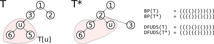
Figure 1. A tree and its dual, along with the BP and DFUDS representations. A subtree $T[u]$ is also highlighted, along with the corresponding nodes in the dual.

Remark 2.3.

It is similarly immediate to observe that there is a well-defined order among nodes that share a parent. It suffices to notice that in $T^{*}$ each node either is a rightmost child (Rules 1b, 3), or it is the (unique) immediate left sibling of another node (Rule 2).

All nodes but $r$ have exactly one (incoming) edge, which implies $|E|=|V|-1$. To conclude that $T^{*}$ is a tree, it remains to show that $T^{*}$ contains no cycles, which we immediately do:

Theorem 2.4.

$T^{*}$ is a well-defined, rooted, ordered tree.

We do this by explicitly specifying the parents of nodes in $T^{*}$, by making use of the depth-first traversal order $<$ in $T$. For this, let $T[v]$ be the subtree of $T$ that hangs off (and includes) $v\in T$, i.e. $T[v]$ contains $v$ and all its descendants in $T$. Let further

$$R[v]:=\{u\in T\setminus T[v]\mid v<u\}$$

be all nodes “right of” $v$ according to depth-first traversal order. For two nodes $u,v$ where $u$ is an ancestor of $v$, we immediately note that

$$T[v]\subset T[u],\quad R[u]\subset R[v]\quad\text{ and }\quad R[v]\subset T[u]\;\cup\;R[u]$$ (10)

For a node $v\in T\setminus\{r\}$, we then obtain the following lemma:

Lemma 2.5.

$$\mathsf{pa}^{*}(v)=\begin{cases}\min R[v]&R[v]\neq\emptyset\\ r&R[v]=\emptyset\end{cases}$$

We refer to Appendix B for the proof of Lemma 2.5. Using Lemma 2.5, a proof of theorem 2.4 can be immediately given:

Proof of Theorem 2.4. Lemma 2.5 implies that $v<_{T}\mathsf{pa}^{*}(v)$ for all $v\in T\setminus\{r\}$. Therefore, $T^{*}$ can contain no cycles and we obtain that $T^{*}$ is a tree as a corollary. Furthermore, lemma 2.5 reveals that $T^{*}$ is unique. ∎

See again Appendix B for immediate corollaries B.1 and B.3 which point out how parents and subtrees in $T^{*}$ relate with one another.

Remark 2.6.

An intuitive guideline for describing $T^{*}$ in comparison to $T$ is that parent- and siblinghood, as well as left and right are exchanged. In other words (and as will become clearer explicitly later) the duality describing $T^{*}$ can be decomposed into two subdualities, one of which turns parents into siblings and vice versa, and the other one of which exchanges left and right.

This remark had left us with some choices for characterizing tree duality. Our choice is motivated by [8], arguably a cornerstone in RMQ theory development. To understand this, let $A=A[1,n]$ be the array, on which RMQ’s are to be run, and let $\overleftrightarrow{A}$ be its reversal, given by $\overleftrightarrow{A}[i]=A[n-i+1]$. Let ${T[A]}$ be the 2D-Min-Heap constructed from $A$, as described in [8] (a definition is provided in Appendix C),

to which RMQ’s refer (see (2),(3),(4)). An immediate question to ask is what RMQ’s would look like when performing RMQ’s on $\overleftrightarrow{A}$ instead of $A$. Here is the answer.

Theorem 2.7.

Let $A[1,N]$ be an array and let $\overleftrightarrow{A}:=[A[N],...,A[1]]$ its reversal. Then

$$({T[A]})^{*}=T[\overleftrightarrow{A}]$$ (11)

An illustration of the Theorem is provided in Figure 2. See Appendix C for a more detailed treatment of this motivating example, including proofs. Thanks to theorem 2.7, the definition of $T^{*}$ can arguably be considered a most natural choice, at least when relating tree duality with RMQ’s.

Figure 2. (left) An array $A$ along with the 2D-Min-Heap ${T[A]}$. Arcs above array indices indicate tree paths. (middle) The dual tree $({T[A]})^{*}$. (right) The reversed array $\overleftrightarrow{A}$ along with the 2D-Min-Heap $T[\overleftrightarrow{A}]$.

Before proceeding with results on succinct tree representations, we provide the following intuitive lemma about the depth-first traversal order of $T^{*}$ as a rooted, ordered tree. This lemma, in combination with lemma 2.5, supports the (intended) intuition that in $T^{*}$ up and down, as well as left and right, are exchanged, properties that are characteristic for rooted, ordered tree duality. It also provides motivation beyond theorem 2.7 in the Introduction why $T^{*}$ is the possibly canonical choice of the dual of a tree.

Therefore, let $<^{*}$ denote the depth-first traversal order in $T^{*}$ (well-defined by theorem 2.4) while $<$ denotes the depth-first traversal order in (the primal tree) $T$.

Lemma 2.8.

Let $u,v\in T\setminus\{r\}$. Then

$$u<^{*}v\quad\text{if and only if}\quad v<u$$

The proof of lemma 2.8 makes use of the following technical lemmata 2.9 and 2.10, which are of use also elsewhere. We therefore state these technical lemmata here. The proofs for all lemmata 2.8, 2.9 and 2.10 can finally be found in Appendix D.

Lemma 2.9.

Let $w:=\mathsf{pa}^{*}(v)$ and $v_{2}\in T[v]\setminus v$ such that $\mathsf{pa}^{*}(v_{2})=w$. Then $v_{2}<^{*}v$.

Lemma 2.10.

Let $v_{1}$ be a sibling left of $u_{1}$ in $T$. Then $T[v_{1}]\subset T^{*}[u_{1}]$.

With lemma 2.8 proven, we can conclude with proving a main theorem of this treatment. It states that the dual of the dual is the primal tree, arguably a key property for a sensibly defined duality. Despite all lemmata raised so far, the proof still entails a few technically more demanding arguments.

Theorem 2.11.

$(T^{*})^{*}=T$

Proof 2.12.

It suffices to show that $\mathsf{pa}^{**}(v)=\mathsf{pa}(v)$, since lemma 2.8 establishes that the order in $(T^{*})^{*}$ agrees with that of $T$. Let $u=\mathsf{pa}(v)$. In Appendix E, we provide a (heavily technical) proof that

$$u=\begin{cases}\min_{<^{*}}R^{*}[v]&R^{*}[v]\neq\emptyset\\ r&R^{*}[v]=\emptyset\end{cases}$$

which completes the proof by applying lemma 2.5.

2.1. Tree Reversal

We bring in another, simpler notion of tree duality, namely that of reversing trees. We will further elucidate what the trees are like when combining tree reversal with the tree duality ($T^{*}$) raised earlier.

Definition 2.13 (Reversed tree).

Let $T$ be a tree. The reversed tree $\overleftrightarrow{T}$ of $T$ is the tree resulting from reversing the order among the children of each node.

Proposition 2.14.

Let $\overleftrightarrow{T}$ be the reversed tree of $T$ and $\overleftrightarrow{T^{*}}$ be the reversed dual of $T$. We define $irs$ (immediate right sibling) and $lmc$ (left-most child) similarly as in Section 1.2.

• $(a)$ The root $r$ of $T$ is also the root of $\overleftrightarrow{T}$.

• $(b)$ Let $u=\mathsf{pa}_{T}(v)$. Then also $u=\mathsf{pa}_{\overleftrightarrow{T}}(v)$.

• $(c)$ Let $u=ils_{T}(v)$. Then $u=irs_{\overleftrightarrow{T}}(v)$.

• $(d)$ The root $r$ of $T$ is also the root of $\overleftrightarrow{T^{*}}$.

• $(e)$ If $v=lmc_{T}(r)$ then also $v=lmc_{\overleftrightarrow{T^{*}}}(r)$, implying in particular that $\mathsf{pa}_{\overleftrightarrow{T^{*}}}(v)=r$.

• $(f)$ If $v=lmc_{T}(u)$ with $u\neq r$, so $v=ils_{\overleftrightarrow{T^{*}}}(u)$, implying that $\mathsf{pa}_{\overleftrightarrow{T^{*}}}(v)=\mathsf{pa}_{\overleftrightarrow{T^{*}}}(u)$.

• $(g)$ If $v=ils_{T}(u)$, then $v=lmc_{\overleftrightarrow{T^{*}}}(u)$, implying that $\mathsf{pa}_{\overleftrightarrow{T^{*}}}(v)=u$.

• $(h)$ $\overleftrightarrow{T^{*}}=\overleftrightarrow{T}^{*}$, that is the reversed dual tree of $T$ is the dual of the reversed tree of $T$.

All of those are, in comparison with statements referring to the definition of the dual tree, rather obvious observations. See Appendix F for the proof.

Since $\overleftrightarrow{T}^{*}$ plays a particular role in the context of our introductory motivation, we give it a particular name: $\hat{T}$.

Definition 2.15 (Reversed dual tree).

Let $T$ be a tree. The tree $\hat{T}:=\overleftrightarrow{T}^{*}$ of $T$ is the dual of the reversed (or the reversed dual) tree of $T$.

Based on proposition 2.14, we realize that $\hat{T}$ can be described as turning leftmost children into immediate left siblings.

Remark 2.16.

Following the arguments provided in [7], it becomes evident that the tree $T$ in use there, on which $\mathrm{BP}(T)$ is constructed, turns indeed out to be $\widehat{{T[A]}}=\overleftrightarrow{{T[A]}^{*}}$.

3. The Primal-Dual Ancestor

The following theorem points out that pairs of nodes have a unique primal-dual ancestor. We will further point out properties of that node.

Theorem 3.1.

Let $v_{1},v_{2}\in T\setminus\{r\}$ be two nodes where $v_{1}\leq v_{2}$. Then there is a unique node $v\in T\setminus\{r\}$ such that $v_{1}\in T^{*}[v]$ and $v_{2}\in T[v]$.

We henceforth refer to this unique node as primal-dual ancestor of $v_{1}$ and $v_{2}$, written $\mathsf{pda}(v_{1},v_{2})$.

Proof 3.2.

Let

$$v:=\max_{<_{T}}\{v_{1}\leq x\leq v_{2}\mid v_{1}\in T^{*}[x]\}$$ (12)

be, relative to depth-first traversal order in $T$, the largest ancestor of $v_{1}$ in $T^{*}$ that precedes $v_{2}$. We claim that $v$ is the unique primal-dual ancestor of $v_{1}$ and $v_{2}$.

By definition, we immediately obtain that $v_{1}\in T^{*}[v]$. To prove $v_{2}\in T[v]$, consider $\mathsf{pa}^{*}(v)$, for which, by choice of $v$, we have that $v_{2}<\mathsf{pa}^{*}(v)$. By lemma 2.5, however, $\mathsf{pa}^{*}(v)$ is the first node in $R[v]$, relative to depth-first traversal order in $T$. Hence, for any $y$ such that $v\leq y<\mathsf{pa}^{*}(v)$, which includes $v_{2}$, it holds that $y\in T[v]$.

It remains to show that $v$ is the only possible primal-dual ancestor. By definition of the primal-dual ancestor, $v$ must be an ancestor of $v_{1}$ in $T^{*}$.

First, consider an ancestor $y$ of $v_{1}$ in $T^{*}$ such that $y<v$. By choice of $v$, it holds that $\mathsf{pa}^{*}(y)\leq v_{2}$, while $\mathsf{pa}^{*}(y)\in R[y]$. This implies that also $v_{2}\in R[y]$, and not $v_{2}\in T[y]$, hence $y$ cannot be a primal-dual ancestor of $v_{1}$ and $v_{2}$.

Second, consider an ancestor $y$ of $v_{1}$ in $T^{*}$ such that $v<y$. Because $v$ is an ancestor of $v_{1}$ in $T^{*}$, and $y$ is larger than $v$, $y$ is also an ancestor of $v$ in $T^{*}$. By lemma 2.5, we know that $y\in R[v]$. This, in combination with $v_{2}\in T[v]$ implies that $v_{2}<y$, hence, $y$ cannot be an ancestor of $v_{2}$ in $T$.

For the following theorem, let

$$\mathrm{depth}_{T}(v_{1},v_{2}):=\min\{\mathrm{depth}_{T}(y)\mid v_{1}\leq y\leq v_{2}\}$$

be the minimal depth of nodes between (and including) $v_{1}$ and $v_{2}$.

Theorem 3.3.

Let $v_{1},v_{2}\in T\setminus\{r\}$ such that $v_{1}<v_{2}$. It holds that

$$\mathsf{pda}(v_{1},v_{2})=\max_{<}\{v_{1}\leq x\leq v_{2}\mid\mathrm{depth}_{T}(x)=\mathrm{depth}_{T}(v_{1},v_{2})\}$$ (13)

That is, according to depth-first traversal order in $T$, the primal-dual ancestor is the greatest node whose $T$-depth is minimal among all nodes between (and including) $v_{1}$ and $v_{2}$.

The proof is based on the following lemma:

Lemma 3.4.

Let $v<w$ such that $w\in T[\mathsf{pa}^{*}(v)]$. Then it holds that

$$\mathrm{depth}_{T}(v,w)=\mathrm{depth}_{T}(\mathsf{pa}^{*}(v))$$ (14)

See Appendix G for a proof of lemma 3.4 and then theorem 3.3.

Note immediately that theorem 3.3 implies that $v$ can be found in O(1) runtime, by performing a range minimum query on the excess array $D$ of $\mathrm{BP}(T)$, defined by $D[x]:=\mathsf{rank}_{1}(x)-\mathsf{rank}_{0}(x)$ where $\mathsf{rank}$ refers to $\mathrm{BP}(T)$. Since $D[x+1]-D[x]\in\{-1,+1\}$, an RMQ on $D$ means performing a $\pm 1$-RMQ, for which convenient solutions exist [1].

Re-interpretation of RMQ’s. Because it was shown [8], that the node in the 2D-Min-Heap ${T[A]}$ that corresponds to the solution of $\mathsf{rmq}_{A}(i,j)$ is given by the right hand side of (13), theorems 3.1 and 3.3 allow for a reinterpretation of an RMQ query $\mathsf{rmq}_{A}(i,j)$ on an array $A$ (without going into details here, because the proof is an easy exercise based on collecting facts from here, [8] and [7]).

1. Determine the node $v$ in ${T[A]}$ corresponding to $i$.

2. Determine the node $w$ in ${T[A]}$ corresponding to $j$.

3. Determine $\mathsf{pda}(v,w)$ in ${T[A]}$; return the corresponding index $i_{o}$.
   

Re-interpretation and improvement of Minimal Length Interval Queries (MLIQ). To illustrate the potential practical benefits of our treatment, we further revisit the problem of minimal length interval queries (MLIQ). The improvements we will be outlining are similar in spirit to the ones delivered in [7]. However, based on our results, they are considerably more convenient to obtain.

Problem 3.5 (MLIQ).

Let $([a_{i},b_{i}])_{i\in\{1,...,n\}},a_{i},b_{i}\in\mathbb{N}$ such that $a_{i}\leq b_{i}$ for all $i\in\{1,...,n\}$ and $a_{i}<a_{j}$ and $b_{i}<b_{j}$ for $i<j$.

• Input: $(a,b)$ such that $a<b$

• Output: The index $i_{0}$ such that $[a_{i_{0}},b_{i_{0}}]$ is the shortest interval that contains $[a,b]$, if such an interval exists.

This problem makes part of other relevant problems, for example the shortest unique interval problem. In this context, a solution for the MLIQ problem was presented in [11] that requires $O(b_{n}\log b_{n})$ space to answer the query in $O(1)$ time. Therefore, the following strategy was suggested.

Let $l_{i}:=|b_{i}-a_{i}+1|$ be the length of the $i$-th interval, $A:=[l_{1},...,l_{n}]$ and ${T[A]}$ the corresponding 2D-Min-Heap.

1. $i_{min}:=\min\{i\mid b_{i}>b\},i_{max}:=\max\{i\mid a_{i}<a\}$; if $i_{max}$ $<$ $i_{min}$ output ’None’.

2. Determine nodes $v,w\in{T[A]}$ corresponding to $i_{min},i_{max}$.

3. Determine $\mathsf{pda}(v,w)\in{T[A]}$; output its index.

The solution presented in [11] can immediately be improved by employing bitmaps for the first step (which, according to [17], requires $O(n\log(b_{n}/n))+o(b_{n})$ space). Steps 2 and 3 then reflect an ordinary RMQ, which can be dealt with following [7]. In terms of query counts, Step 1 reflects two $\mathsf{rank}$ queries, while the resulting RMQ, following [7], requires two $\mathsf{select}$’s, one $\pm 1$-$\mathsf{rmq}$, and one $\mathsf{rank}$.

If $|a_{i}-a_{i-1}|,|b_{i}-b_{i-1}|$ are in $O(\log n)$ (which applies for several important applications), further improvements can be made based on suggestions made in [19] for BP representations of trees with weighted parentheses. For that, we construct $T_{a}={T[A]}$ and $T_{b}=\overleftrightarrow{{T[A]}}$. We then assign weights $w_{a,i}:=|a_{i}-a_{i-1}|$ to $i+1$-st opening parenthesis in $T_{a}$, whereas in $T_{b}$ we assign $w_{b,i}:=|b_{i}-b_{i-1}|$ to the $i$-th closing parentheses (where $a_{0}=b_{0}=0$; we recall that the number of non-root nodes in ${T[A]}$ is $n$). When aiming at running queries presented in [19], this requires $2n\log\log n+o(n)$ bits of space, an improvement over $O(n\log(b_{n}/n))+o(b_{n})$ for the above, naive approach. Following [19], let $\mathsf{bpselect}_{w_{a},0}(a),\mathsf{bpselect}_{0,w_{b}}(b)$ be defined by selecting the largest index in the balanced parenthesis vector such that adding up all weights attached to opening parentheses ($w_{a}$) is at most $a$, or adding up all weights attached to closing parentheses ($w_{b}$) is at most $b$. We can then run

1. $w:=\mathsf{bpselect}_{w_{a},0}(a)$ in $T_{a}$ and $v:=2n-\mathsf{bpselect}_{0,w_{b}}(b)+3$ in $T_{b}$; if $v>w$ output ’None’

2. Determine $\mathsf{pda}(v,w)\in T_{a}$; output its index.

In comparison to the naive approach from above, this makes two $\mathsf{bpselect}$ queries, instead of two $\mathsf{rank}$’s and two $\mathsf{select}$’s. The decisive trick is to place $a$ and $b$ directly into ${T[A]}$, which avoids determining indices $i_{min},i_{max}$ first, which subsequently need to be placed. Beyond the improvements in terms of space and query counts, we argue that this solution reflects all symmetries inherent to the MLIQ problem in a particularly compact manner.

4. Relating BP and DFUDS representations

We will use the following construction to set up a tree induction for proving our main theorem.

Definition 4.1 (Tree joining operation).

Let $T_{1}$ and $T_{2}$ be two trees, let $r_{2}$ be the root of $T_{2}$, $rmc_{T_{2}}(r_{2})$ needs to exist and be a leaf. The notation ${T_{1}\curvearrowright T_{2}}$ will denote a new tree formed by taking $T_{2}$ and inserting the children of the root of $T_{1}$ as children of the rightmost child of the root of the new tree. Extend this operation to $n$ trees ${T_{1},\ldots,T_{n}}$ where $T_{2},\ldots,T_{n}$ all satisfy the same property as $T_{2}$ above, in the following way: ${T_{1}\curvearrowright T_{2}\curvearrowright T_{3}}={(T_{1}\curvearrowright T_{2})\curvearrowright T_{3}}$ and so on,

$${T_{1}\curvearrowright T_{2}\ldots\curvearrowright T_{n}}={((\ldots((T_{1}\curvearrowright T_{2})\curvearrowright T_{3})\curvearrowright\ldots)\curvearrowright T_{n})}.$$

Observation 1.

Let $T$ be a tree such that its root $r$ has a single child $c$ (that may or may not be a leaf). Then in $T^{*}$, by Rule 1b, $rmc_{T^{*}}(r)=c$ and is a leaf.

The following Lemma (proven in Appendix H)

relates the dual tree to the tree joining operation. We will use the $r\rightarrow T$ notation to denote a new tree formed by adding a new root $r$ as a parent of the root of $T$.

Lemma 4.2.

Let $T$ be a tree consisting of a root $r$ and $n\geq 1$ subtrees $A_{1},A_{2},\ldots,A_{n}$ as children. When $n=1$, $T^{*}$ is $(r\rightarrow A_{1})^{*}$. When $n\geq 2$, $T^{*}$ is $(r\rightarrow A_{1})^{*}\curvearrowright(r\rightarrow A_{2})^{*}\curvearrowright\ldots\curvearrowright(r\rightarrow A_{n})^{*}$.

We are now ready to prove Theorem 1.1. Parentheses in $\mathrm{BP}$ and $\mathrm{DFUDS}$ representations will be denoted by $\underline{(}$ and $\underline{)}$ to avoid confusion with usual mathematical parentheses. Recall that we use $\overleftrightarrow{s}$ to mirror a string $s$ of parentheses, e.g. $\overleftrightarrow{\underline{(()}}=\underline{())}$ and $\overleftrightarrow{\underline{)()}}=\underline{()(}$.

Proof 4.3 (Proof of Theorem 1.1).

Let $T$ be a tree with $n$ subtrees $A_{1},\ldots,A_{n}$. It is clear that $\mathrm{BP}(T)=\underline{(}\mathrm{BP}(A_{1})\mathrm{BP}(A_{2})\ldots\mathrm{BP}(A_{n})\underline{)}$. Observe that for two trees $T_{1}$ and $T_{2}$ with roots $v_{1}$ and $v_{2}$, and where $rmc_{T_{1}}(v_{1}),rmc_{T_{2}}(v_{2})$ both exist and are leaves,

$$\mathrm{DFUDS}(T_{1}\curvearrowright T_{2})=\underline{(}\mathrm{DFUDS}(T_{2}\setminus rmc_{T_{2}}(v_{2}))\mathrm{DFUDS}(T_{1}\setminus rmc_{T_{1}}(v_{1}))\underline{)}.$$

In fact, one can show recursively that such a decomposition can be extended to $T_{1}\curvearrowright\ldots\curvearrowright T_{n}$. We will now prove the theorem with a tree structural induction. Observe that for a tree $T$ of depth 1 (a single root node),

$$\mathrm{BP}(T)=\underline{()}=\mathrm{DFUDS}(T^{*})=\overleftrightarrow{\mathrm{DFUDS}(T^{*})}.$$

Now, assume the theorem equality is true for trees of depth $i$ and we will show it for trees of depth $i+1$. A tree $T$ of depth $i+1$ can be decomposed into a root node $r$ and $n$ subtrees $A_{1},\ldots,A_{n}$ that are all of of depth $\leq i$ with roots $a_{1},\ldots,a_{n}$. Using Lemma 4.2,

$$\mathrm{DFUDS}(T^{*})=\mathrm{DFUDS}((r\rightarrow A_{1})^{*}\curvearrowright(r\rightarrow A_{2})^{*}\curvearrowright\ldots\curvearrowright(r\rightarrow A_{n})^{*}).$$

By the recursive decomposition that we observed above, and using Observation 1 stating that the rightmost child of $r$ in $(r\rightarrow A_{i})^{*}$ is a leaf,

$$\mathrm{DFUDS}(T^{*})=\underline{(}\mathrm{DFUDS}((r\rightarrow A_{n})^{*}\setminus\{a_{n}\})\ldots\mathrm{DFUDS}((r\rightarrow A_{1})^{*}\setminus\{a_{1}\})\underline{)}.$$

Observe that we can take each DFUDS term in the expression above and wrap it around parentheses, i.e. $\underline{(}\mathrm{DFUDS}((r\rightarrow A_{i})^{*}\setminus\{a_{i}\}\underline{)}$ which is equal to $\mathrm{DFUDS}((r\rightarrow A_{i})^{*})$. Furthermore, note the following identity: $\mathrm{DFUDS}((r\rightarrow A_{i})^{*})=\underline{(}\mathrm{DFUDS}(A_{i}^{*})\underline{)}$. And by inductive hypothesis, $\mathrm{DFUDS}(A_{i}^{*})=\overleftrightarrow{\mathrm{BP}(A_{i})},$ thus $\mathrm{DFUDS}((r\rightarrow A_{i})^{*}\setminus\{a_{i}\})=\overleftrightarrow{\mathrm{BP}(A_{i})}$. Hence,

$$\overleftrightarrow{\mathrm{DFUDS}(T^{*})}=\underline{(}\mathrm{BP}(A_{1})\ldots\mathrm{BP}(A_{n})\underline{)}=\mathrm{BP}(T).$$

Proving (7) from the Introduction. Eventually, we also realize that $\mathrm{BP}(\overleftrightarrow{T})=\overleftrightarrow{\mathrm{BP}(T)}$ and also $\mathrm{DFUDS}(\overleftrightarrow{T})=\overleftrightarrow{\mathrm{DFUDS}(T)}$, both of which is straightforward [$\star$]. Using this in combination with theorems 2.11 and 1.1, we obtain

$$\mathrm{DFUDS}({T[A]})\stackrel{{\scriptstyle[\star]}}{{=}}\overleftrightarrow{\mathrm{DFUDS}(\overleftrightarrow{{T[A]}})}\stackrel{{\scriptstyle Th.\ref{t.dualdual}}}{{=}}\overleftrightarrow{\mathrm{DFUDS}((\overleftrightarrow{{T[A]}}^{*})^{*})}\stackrel{{\scriptstyle Th.\ref{thm:bpdfuds}}}{{=}}\mathrm{BP}(\overleftrightarrow{{T[A]}}^{*})\stackrel{{\scriptstyle D.\ref{d.reversedual}}}{{=}}\mathrm{BP}(\widehat{{T[A]}})$$

which establishes equation (7) from the introduction.

Conclusive Remarks. In summary, we have provided a framework that unifies $\mathrm{BP}$ and $\mathrm{DFUDS}$. From a certain point of view, we have pointed out that neither should $\mathrm{BP}$ based approaches have advantages over $\mathrm{DFUDS}$ based approaches, nor vice versa. As an exemplary perspective of our framework, $\mathrm{BP}$ based treatments such as [16, 19] might have an easier grasp of the advantages that $\mathrm{DFUDS}$ based approaches bring along. Finally, we consider it interesting future work to also characterize trees that put $\mathrm{BP}$ and/or $\mathrm{DFUDS}$ based representations into context with $\mathrm{LOUDS}$ based representations.

Appendix A The simpler query from [7] also works in [8]: direct proof

In the following, we identify nodes of $T$ with the closing parenthesis that represent them in $\mathrm{DFUDS}$, that is $v=\mathrm{CP}(v)$. Recall that $D$ is the array defined in Section 1.

Lemma A.1.

Let $v_{2}$ the immediate right sibling of $v_{1}$. Then, in $\mathrm{DFUDS}(T)$,

$$D[v_{2}]=D[v_{1}]-1$$ (15)

Proof A.2.

Given (15), we show that all parentheses between $v_{1}$ and $v_{2}$ are elements of $T[v_{1}]$, the subtree hanging off (but here not including) $v_{1}$. In other words, we will show that

$$x\in T[v_{1}]\quad\text{if and only if}\quad v_{1}<v<v_{2}$$ (16)

For “$\Rightarrow$”, the first case is that $v$ represents a closing parenthesis. Then the claim follows because closing parentheses come in depth-first traversal order, hence $v$ comes after $v_{1}$, and before $v_{2}$. The second case is that $v$ represents an opening parenthesis. So, by $\mathrm{DFUDS}$ principles, the first closing parenthesis to the left of $v$ refers to $v$’s parent, which is either itself a member of $T[v_{1}]$ or $v_{1}$ itself. In both cases, $x$ comes after $v_{1}$ and before $v_{2}$.

For “$\Leftarrow$”, the case of $v$ being a closing parenthesis implies the claim because of the depth-first traversal order. The case of $v$ being an opening parenthesis requires to look at the first closing parenthesis $u$ to the left, which refers to the parent of $v$. We obtain $\{v\}\subset T[u]\subset T[v_{1}]$, because $u$ either is a descendant of $v_{1}$ or $v_{1}$ itself.

Lemma A.3.

Let $v_{2}$ be the rightmost child of $v_{1}$. Then, in $\mathrm{DFUDS}(T)$,

$$D[v_{2}]=D[v_{1}]$$

Proof A.4.

By $\mathrm{DFUDS}$ logic, $\mathrm{OP}(v_{2})$ directly follows $v_{1}$. Further, again by $\mathrm{DFUDS}$ logic, the parentheses between $\mathrm{OP}(v_{2})$ and $v_{2}$ are exactly the members of subtrees of all children of $v_{1}$, but $v_{2}$. That is, we are facing the following situation:

$$\underset{v_{1}}{\big{)}}\;\underset{\mathrm{OP}(v_{2})}{\big{(}}\;\underset{T[v_{1}]\setminus T[v_{2}]}{\underbrace{\big{(}...............\big{)}}}\quad\underset{v_{2}}{\big{)}}\quad\underset{T[v_{2}]}{\underbrace{\big{(}......}}$$ (17)

So, $D[v_{2}-1]=D[\mathrm{OP}(v_{2})]$, and further $D[v_{2}]=D[v_{2}-1]-1$ and $D[v_{1}]=D[\mathrm{OP}(v_{2})]-1$, which together implies

$$D[v_{2}]=D[v_{2}-1]-1=D[\mathrm{OP}(v_{2})]-1=D[v_{1}]$$ (18)

To provide a direct proof of the fact that Ferrada and Navarro’s query also works for Fischer and Heun, we have to show that in $\mathrm{DFUDS}({T[A]})$,

$$\mathsf{rank}_{)}(\mathsf{open}(w_{1}))=i$$

is equivalent to

$$\mathsf{rmq}_{D}(\mathsf{select}_{)}(i),\mathsf{select}_{)}(j))=\mathsf{select}_{)}(i)$$

Recalling that $\mathsf{rmq}_{D}$ refers to the leftmost minimum in the array $D$, where $D[x]=\mathsf{rank}_{1}(x)-\mathsf{rank}_{0}(x)$ for a parenthesis $x\in\mathrm{DFUDS}({T[A]})$, we have to prove the following technical lemma.

Lemma A.5.

In $\mathrm{DFUDS}(T)$, the following two statements are equivalent:

• $(i)$

  $$\text{For all}\quad x\in[\mathsf{select}_{0}(i+1),\mathsf{select}_{0}(j)]:\quad D[\mathsf{select}_{0}(i)]\leq D[x]$$ (19)

• $(ii)$

  $$\mathsf{rank}_{0}(\mathsf{open}(\mathsf{rmq}_{D}(\mathsf{select}_{0}(i+1),\mathsf{select}_{0}(j))))=i$$ (20)

Proof A.6.

$(i)\Rightarrow(ii)$: By lemmata A.1 and A.3, we know that the first parenthesis $x$ right of $\mathsf{select}_{0}(i)$ where $D[x]<D[\mathsf{select}_{0}(i)]$ is the sibling right of the node $v$ represented by $\mathsf{select}_{0}(i)$. Hence by $\mathrm{DFUDS}$ logic, $(i)$ implies that all $x\in[\mathsf{select}_{0}(i+1),\mathsf{select}_{0}(j)]$ refer to descendants of $v$. Again using lemmata A.1 and A.3, we infer that $w_{1}:=\mathsf{rmq}_{D}(\mathsf{select}_{0}(i+1),\mathsf{select}_{0}(j))$ refers to the closing parenthesis of the rightmost child of $v$ among the children of $v$ showing in $[\mathsf{select}_{0}(i+1),\mathsf{select}_{0}(j)]$—note that there is at least one, because $\mathsf{select}_{0}(i+1)$ refers to the leftmost child of $v$. So, $\mathsf{open}(w_{1})$ is one of the opening parentheses directly following $\mathsf{select}_{0}(i)$, that is $\mathsf{rank}_{0}(w_{1})=\mathsf{rank}(\mathsf{select}_{0}(i))=i$.

$(ii)\Rightarrow(i)$: If $(ii)$ applies, $w_{1}:=\mathsf{rmq}_{D}(\mathsf{select}_{0}(i+1),\mathsf{select}_{0}(j))$ is a closing parenthesis whose opening counterpart follows $\mathsf{select}_{0}(i)$ without any closing parenthesis in between. That is, $w_{1}$ represents one of the children of $\mathsf{select}_{0}(i)$. From lemmata A.1 and A.3, we infer that $D[\mathsf{select}_{0}(i)]\leq D[w_{1}]$ with equality if and only if $w_{1}$ represents the rightmost child of $\mathsf{select}_{0}(i)$. Because $D[w_{1}]$ was selected as the minimum among the $D[x],x\in[\mathsf{select}_{0}(i+1),\mathsf{select}_{0}(j)]$, we obtain

$$D[\mathsf{select}_{0}(i)]\leq D[w_{1}]\leq D[x]$$ (21)

Appendix B Proof of Lemma 2.5 and Corollaries B.1, B.3

Proof of Lemma 2.5. We consider the three different cases that correspond to Rules 1b, 3 and 2 (in that order).

Ad Rule 1b: If $v$ is the rightmost child of the root, all nodes that follow $v$ in depth-first traversal order are in the subtree $T[v]$ of $v$, so $R[v]$ is the empty set.

Ad Rule 3: If $v=ils_{T}(u)$, then $u$, in depth-first traversal order, is the first node following nodes in $T[v]$, the subtree of $v$, that is, $u$ is the smallest node in $R[v]$, so $\mathsf{pa}^{*}(v)=u$.

Ad Rule 2: Here, $v=rmc_{T}(u)$. We lead the proof by induction on $\mathrm{depth}_{T}(v)$, where the start, $\mathrm{depth}_{T}(v)=1$, is given by the already proven case of Rule 1b. Let $i\geq 1$ and $\mathrm{depth}_{T}(v)=i+1$. As $\mathsf{pa}_{T}(v)=u$, it holds that $\mathrm{depth}_{T}(u)=i$, so by the induction assumption, in combination with $\mathsf{pa}^{*}(u)=\mathsf{pa}^{*}(v)$, we obtain

$$\mathsf{pa}^{*}(v)=\begin{cases}r&R[u]=\emptyset\\ \min R[u]&R[u]\neq\emptyset\end{cases}.$$ (22)

Case 1, $R[u]=\emptyset$: $v$ being a child of $u$ implies $T[v]\subset T[u]$. The assumption $R[v]\neq\emptyset$ would imply the existence of a node $x$ right of $v$. Since $R[u]=\emptyset$, we obtain by (10) that $R[v]\subset T[u]$, so $x\in T[u]$. The combination of $x$ being right of $v$ and being part of the subtree $T[u]$ rooted at the parent $u$ of $v$ implies the existence of a right sibling of $v$, which is a contradiction to $v=rmc_{T}(u)$.

Case 2, $R[u]\neq\emptyset$: Let $x:=\mathsf{pa}^{*}(v)=\min R[u]$ and let $y:=\min R[v]$. We need to show that $x=y$. Because of (10), we know that $y\leq x$. The assumption $y<x$, however, implies the existence of a node right of $v$ that lies in $T[u]$, which again contradicts $v=rmc_{T}(u)$.∎

Corollary B.1.

Let $u$ be an ancestor of $v$ in $T$. Then

$$\mathsf{pa}^{*}(v)\leq_{T}\mathsf{pa}^{*}(u).$$

Proof B.2.

This follows from lemma 2.5 in combination with (10), where the latter states that $R[u]\subset R[v]$, making $\min R[v]\leq_{T}\min R[u]$.

The next corollary is an immediate consequence of corollary B.1.

Corollary B.3.

Let $w=\mathsf{pa}^{*}(v)$ for $v\in T\setminus\{r\}$. Then

$$T[v]\subset T^{*}[w].$$

Proof B.4.

Let $v_{2}\in T[v]$, that is $v$ is an ancestor of $v_{2}$ in $T$. We have to show that $w$ is an ancestor of $v_{2}$ in $T^{*}$. From corollary B.1, we know that $\mathsf{pa}^{*}(v_{2})\leq_{T}\mathsf{pa}^{*}(v)$, so, because $\mathsf{pa}^{*}(v)$ is the first node in $T$-order not in $T[v]$, either $\mathsf{pa}^{*}(v_{2})=\mathsf{pa}^{*}(v)$ or $\mathsf{pa}^{*}(v_{2})\in T[v]$. In the first case, we are done. In the second case, we repeat this argument by replacing $v_{2}$ with $\mathsf{pa}^{*}(v_{2})$ (formally: induction on the number of nodes between $v_{2}$ and $\mathsf{pa}^{*}(v)$ in $T$-order) to conclude the proof.

Appendix C Proof of Theorem 2.7.

Here, we provide a proof for our motivating theorem 2.7. Le $A=A[1,n]$ be an array. For additional clarity, we require $S_{A}:=\{A[1],...,A[n]\}$ to form a totally ordered set, implying that for all $i\neq j,1\leq i,j\leq n$, either $A[i]<A[j]$ or $A[j]<A[i]$, and note that this requirement can easily be overcome in applications. As before, $\overleftarrow{A}$ is the reversal $A$, given by $\overleftarrow{A}[i]:=A[N-i+1]$.

We will deal with two orderings in the following, namely, the one on the list indices $\{1,...,N\}$ and the one on the set $S_{A}:=\{A[1],...,A[N]\}$. If distinction is required, we write $<_{A}$ for the former and $<_{S}$ for the latter.

Definition C.1.

(from [8]) The 2D-Min-Heap ${T[A]}$ for an array $A[1,N]$ is a rooted, ordered tree where, first,

$$V\setminus r=\{A[1],...,A[N]\}.$$

Edges are determined by way of iteratively determining the parent of $A[m+1]$ in $T_{A[1,m]}$:

1. The parent of $A[1]$ is $r$.

2. Let $T_{A[1,m]}$ be already constructed. Then $A[m+1]=rmc(A[k])$ where $k:=\max_{<_{A}}\{l\in\{1,...,m\}\mid A[l]<_{S}A[m+1]\}$.

That is, $A[m+1]$ is appended as the rightmost child to the rightmost element in $A[1,m]$ that is smaller than $A[m+1]$.

We make some observations leading to a characterization of the depth-first traversal order on ${T[A]}$, all of which are straightforward (and well known).

Observation 2.

Let $A[k]<_{S}A[i]$ for all $k+1\leq i\leq k+l$. Then $A[i]\in{T[A]}[A[k]]$ for all $k+1\leq i\leq k+l$

Proof of Observation 2. One obtains this insight by induction on $i$. By construction of ${T[A]}$, we obtain that $A[k+1]$ is appended to $T_{A[1,k]}$ as rightmost child of $A[k]$, which makes the start. Consider $A[k+i+1]$ for $1\leq i\leq l-1$. Since $A[k]<A[k+i+1]$, the parent of of $A[k+i+1]$ is one of the $A[k],...,A[k+i]$. By the induction assumption, that parent is an element of ${T[A]}[A[k]]$, so also $A[k+i+1]\in{T[A]}[A[k]]$. ∎

Observation 3.

Let $A[m]\in{T[A]}[A[k]]$. Then $A[k]<_{S}A[m]$.

Proof of Observation 3. This insight is an immediate consequence following from the fact that a node $A[j]$ is greater than its parent $A[i]$, that is, $A[j]<_{S}A[i]$. ∎

With these observations at hand, we can prove the following (well-known, intuitively straightforward) lemma.

Lemma C.2.

The depth-first traversal order $<_{{T[A]}}$ on ${T[A]}$ coincides with the order $<_{L}$ on $\{1,...,N\}$. That is, for $i,j\in\{1,...,N\}$

$$i<j\quad\text{ if and only if }\quad A[i]<_{{T[A]}}A[j].$$

Proof of Lemma C.2. Let $1\leq i\leq N-1$. It suffices to show that $A[i+1]$ comes after $A[i]$ in depth-first traversal order on ${T[A]}$. Therefore, let $A[k]:=\mathsf{pa}_{{T[A]}}(A[i+1])$. If $k=i$, hence $A[k]=A[i]$, we are done. If not, consider all nodes $A[k+1],...,A[i]$ between $A[k]$ and $A[i+1]$. By construction of ${T[A]}$, we know that $A[i+1]<_{S}A[j]$ for all $k+1\leq j\leq i$, while $A[k]<_{S}A[i+1]$, which implies that $A[k]<_{S}A[j]$ for all $k+1\leq j\leq i$. So, by observation 2, all $A[j]\in T[A[k]]$ for $k+1\leq j\leq i$, implying in particular that $A[i]\in T[A[k]]$. Since during construction of ${T[A]}$ $A[i+1]$ is appended as rightmost child of $A[k]$ after $A[i]$ had been appended, $A[i+1]$ comes after $A[i]$ in depth-first traversal order on ${T[A]}$. ∎

We are now in position to prove theorem 2.7.

Theorem C.3.

Let $A[1,N]$ be an array of (mutually different) numbers and let $\overleftarrow{A}:=[A[N],...,A[1]]$ be the reversal of it. Then

$$({T[A]})^{*}={T[\overleftarrow{A}]}.$$ (23)

Proof C.4.

By applying lemma C.2 for ${T[\overleftarrow{A}]}$, the depth-first traversal order on nodes in ${T[\overleftarrow{A}]}\setminus r$ agrees with the reverse order on $\{1,...,N\}$. By applying lemma C.2 for ${T[A]}$ and combining it with lemma 2.8 for ${T[A]}$, we see that the depth-first traversal order on ${T[\overleftarrow{A}]}$ agrees with that on ${T[A]}^{*}$.

It remains to show that the parent of $A[k]$ in $({T[A]})^{*}$ agrees with the parent of $A[k]$ in ${T[\overleftarrow{A}]}$. We recall lemma 2.5 and know that $\mathsf{pa}_{({T[A]})^{*}}(A[k])=r$ if $R_{{T[A]}}[A[k]]=\emptyset$ (first case) and $\mathsf{pa}_{({T[A]})^{*}}(A[k])=\min_{<_{{T[A]}}}R_{{T[A]}}[A[k]]$ if $R_{{T[A]}}[A[k]]$ is not empty (second case).

For the first case, we are done if $A[k]=A[N]$, because then $\mathsf{pa}_{{T[\overleftarrow{A}]}}(A[N])=r$ by construction of ${T[\overleftarrow{A}]}$. If not, $R_{{T[A]}}[A[k]]=\emptyset$ translates into $A[i]\in T[A[k]]$ for $k+1\leq i\leq N$. That is, when constructing ${T[\overleftarrow{A}]}$, there is no node in $T[[A[N],...,A[k+1]]]$ that is smaller than $A[k]$, in which case $A[k]$ is appended to $T[[A[N],...,A[k+1]]]$ as the rightmost child of the root, so also here $\mathsf{pa}_{{T[\overleftarrow{A}]}}(A[N])=r$.

In the second case, we consider $A[l]:=\min_{{T[A]}}R_{{T[A]}}[A[k]]$, the parent of $A[k]$ in $({T[A]})^{*}$. So, by definition of $R_{{T[A]}}[A[k]]$, we have that $A[i]\in{T[A]}[A[k]]$ for all $i:k+1\leq i\leq l-1$. So, by observation 3, $A[k]<A[i]$ for all $i:k+1\leq i\leq l-1\;(\star)$.

Furthermore, $A[l]\in R_{{T[A]}}[A[k]]$ translates into the fact that $A[l]$, during the construction of ${T[A]}$, was not appended to a child of any of the nodes in ${T[A]}[A[k]]$, so $A[l]<A[i]$ for all nodes $A[i]\in{T[A]}[A[k]]$, which implies in particular that $A[l]<A[k]\;(\star\star)$.

So, when appending $A[k]$ to $T[[A[N,...,A[k+1]]]$ during the construction of ${T[\overleftarrow{A}]}$, combining $(\star)$ and $(\star\star)$ yields that $A[l]$ was found to be the rightmost element in $[A[N,...,A[k+1]]$ that was smaller than $A[k]$, which agrees with the definition of the parent of $A[k]$ in ${T[\overleftarrow{A}]}$.

Appendix D Proofs of Lemmata 2.8, 2.9, 2.10

Proof of Lemma 2.9. The edge $(w,v_{2})$ in $T^{*}$ cannot be due to Rule 3, because $v_{2}$ is not the immediate left sibling of $w$ in $T$, which would imply that $w\in T[v]$, which contradicts $w\in R[v]$ or $w$ being the root, which is established by $w=\mathsf{pa}^{*}(v)$ and lemma 2.5.

Note that, since $v$ is not the root, also Rule 1b does not apply. So the edge $(w,v_{2})$ in $T^{*}$ must have come into existence by Rule 2. That is, $v_{2}=ils_{T^{*}}(v_{3})$ where $v_{2}$ was the rightmost child of $v_{3}$ in $T$. We have $v_{3}\in T[v]$ and $\mathsf{pa}^{*}(v_{3})=w$. We are done if $v_{3}=v$, because then $v_{2}$ is the immediate left sibling of $v$ in $T^{*}$. If not, we obtain the claim by induction on $\mathrm{depth}(v_{2})-\mathrm{depth}(v)$. ∎

Proof of Lemma 2.10. By Rule 3, we know that the immediate right sibling $v_{2}$ of $v_{1}$ in $T$ is the parent of $v_{1}$ in $T^{*}$, in other words, $v_{2}=\mathsf{pa}^{*}(v_{1})$. Corollary B.3 implies that $T[v_{1}]\subset T^{*}[v_{2}]$, so we are done if $v_{2}=u_{1}$. If not, then repeated application of Rule 3 implies that $u_{1}$ is an ancestor of $v_{2}$ in $T^{*}$. In other words, $v_{2}\in T^{*}[u_{1}]$, hence also $T^{*}[v_{2}]\subset T^{*}[u_{1}]$, which finally yields $T[v_{1}]\subset T^{*}[u_{1}]$, as claimed. ∎

We can now proceed with proving lemma 2.8.

Proof of Lemma 2.8. It suffices to show that $v<u$ implies $u<^{*}v$. If $v<u$, two different cases can apply, either $u\in T[v]$ or $u\in R[v]$.

Ad $u\in T[v]$: Let $w:=\mathsf{pa}^{*}(v)$. Corollary B.3 implies that $w$ is an ancestor of $u$. Since all ancestors of $u$ in $T^{*}$ are greater than $v$ in terms of depth-first traversal order in $T$, we obtain the existence of a node $v_{2}>v$ such that $\mathsf{pa}^{*}(v_{2})=w$ where, possibly, $v_{2}=u$ itself. We obtain the claim by applying lemma 2.9.

Ad $u\in R[v]$: Let $w$ be the least common ancestor of $v$ and $u$ in $T$ and let $v_{1},u_{1}$ be the children of $w$ such that $v\in T[v_{1}]$ and $u\in T[u_{1}]$. By the prior case $u\in T[v]$, we know that $u<^{*}u_{1}$. Application of lemma 2.10 then further yields that $u_{1}<^{*}v$, which implies the desired $u<^{*}v$. ∎

Appendix E Proof of Theorem 2.11.

We first consider the case $R^{*}[v]=\emptyset$. Here, by depth-first traversal order in $T^{*}$, all ancestors $v_{1}<^{*}...<^{*}v_{l}<^{*}v$ of $v$ (apart from the root $r$) and $v$ are rightmost children. By repeated application of Rule 3, we see that all nodes $v_{1}>...>v_{l}>v$ are siblings in $T$, where $v$ is the leftmost. So, the parent of $v$ agrees with the parent of $v_{1}$, which is the rightmost child of the root $r$. By Rule 1b, we see that also in $T$, the parent of $v_{1}$ is the root $r$.

We now consider the case $R^{*}[v]\neq\emptyset$. First, $u<v$ implies $v<^{*}u$ using lemma 2.8. The assumption $u\in T^{*}[v]$ implies that $v$ is an ancestor of $u$ in $T^{*}$, which is impossible, because lemma 2.5 then says that $v\not\in T[u]$. So $u\in R^{*}[v]$, and it remains to show that $u$ is the smallest node in $R^{*}[v]$, according to $<^{*}$.

We assume the existence of $x\in R^{*}[v]$ that is smaller than $u$, and show that this leads to a contradiction. By lemma 2.8, this implies that $u<x$, so either (1) $x\in T[u]$ or (2) $x\in R[u]$.

Ad (1): For $x\in T[u]$, let $x_{1}$ be the child of $u$, such that $x\in T[x_{1}]$. If $x_{1}$ is a left sibling of $v$, we obtain $x\in T[x_{1}]\subset T^{*}[v]$ by lemma 2.10, a contradiction to $x\in R^{*}[v]$. If $x_{1}$ is a right sibling of $v$, we obtain $v\in T^{*}[x_{1}]$, again by lemma 2.10, which implies $x_{1}<^{*}v$. Further, $x\in T[x_{1}]$ implies $x_{1}<x$, and further into $x<^{*}x_{1}$ by lemma 2.8. Together, we obtain $x<^{*}v$, a contradiction to $x\in R^{*}[v]$.

Ad (2): It remains to consider the case $x\in R[u]$. By depth-first traversal order in $T$, we have $u<v<x$, so in $T^{*}$, by lemma 2.8, $x<^{*}v<^{*}u$. This contradicts that $x\in R^{*}[v]$, which concludes the proof. ∎

Appendix F Proof of Proposition 2.14

Note that $(a)-(c)$ are immediate. For $(d)-(g)$ note that rules for $\overleftrightarrow{T^{*}}$ basically reiterate the rules for the dual tree, while exchanging left with right.

Proof F.1.

Again, these are straightforward observations, obtained by reversing the order among the children of nodes in $T^{*}$, which yields, as one example, that in $\overleftrightarrow{T^{*}}$, the immediate left sibling $v$ of $u$ in $T$ turns into the rightmost child of $u$ in $T^{*}$, which by reversing $T^{*}$ turns into the leftmost child of $T^{*}$, and so on. Computing $\overleftrightarrow{T}^{*}$, the dual of the reversed tree, we find that $(d)-(g)$ apply also for $\overleftrightarrow{T}^{*}$, just as for $\overleftrightarrow{T^{*}}$. Since one can show that $(d)-(g)$ are defining properties of $\overleftrightarrow{T^{*}}$, in analogy to the insight that rules 1-3 from Definition 2.1 give rise to the dual tree $T^{*}$ itself, we see that $\overleftrightarrow{T}^{*}$ and $\overleftrightarrow{T^{*}}$ must be identical.

Appendix G Proof of Lemma 3.4 and Theorem 3.1.

In the following, we write $\mbox{\rm dist}_{T}(v,w)$ and $\mbox{\rm dist}_{T^{*}}(v,w)$ for the length of a minimum length path between $v$ and $w$ in $T$ and $T^{*}$, respectively. We will also write $y=(\mathsf{pa})^{i}(v)$ and $y=(\mathsf{pa}^{*})^{i}(v)$ if $y$ is the $i$-th ancestor of $v$ in $T$ or $T^{*}$, respectively.

In the following, ’first’, ’largest’, and so on, refer to depth-first traversal order in $T$. When referring to depth-first traversal order in $T^{*}$, we will explicitly mention this.

For the proofs, we recall that

$$\mathrm{depth}_{T}(v_{1},v_{2}):=\min\{\mathrm{depth}_{T}(y)\mid v_{1}\leq y\leq v_{2}\}$$

is the minimal depth of nodes between (and including) $v_{1}$ and $v_{2}$. We then observe the following relationship for $v_{1}\leq w\leq v_{2}$:

$$\mathrm{depth}_{T}(v_{1},v_{2})=\min(\mathrm{depth}_{T}(v_{1},w),\mathrm{depth}_{T}(w,v_{2}))$$ (24)

Proof of Lemma 3.4. First, all nodes that follow $\mathsf{pa}^{*}(v)$ in depth-first traversal order until $w$ are in $T[\mathsf{pa}^{*}(v)]$, hence have depth greater than $\mathsf{pa}^{*}(v)$. Second, by lemma 2.5, all nodes between $v$ and $\mathsf{pa}^{*}(v)$ are members of $T[v]$, hence have greater depth than $v$. The dual parent $\mathsf{pa}^{*}(v)$ of $v$, by lemma 2.5 the first node in $R[v]$ following the nodes in $T[v]$ is either a right sibling of $v$ or a right sibling of one of the ancestors of $v$, all of which is a direct consequence of depth-first traversal order. Either way, $\mathrm{depth}_{T}(\mathsf{pa}^{*}(v))\leq\mathrm{depth}_{T}(v)$.∎

Proof of Theorem 3.1. Let $v:=\mathsf{pda}(v_{1},v_{2})$. We encounter the following situation: $v$ is the largest node smaller or equal to $v_{2}$ that is a $T^{*}$-ancestor of $v_{1}$. So, in particular, $\mathsf{pa}^{*}(v)>v_{2}$. By lemma 2.5, $\mathsf{pa}^{*}(v)$ is the first node following $v$ that is not in the subtree $T[v]$ rooted at $v$. So, all nodes following $v$, until and including $v_{2}$ are in $T[v]$, hence have depth larger than $v$. That is,

$$\mathrm{depth}_{T}(v,v_{2})=\mathrm{depth}_{T}(v),$$ (25)

Further, again by lemma 2.5, $\mathsf{pa}^{*}(y)$ is the first node following $y$ that is not in $T[y]$. Hence, by definition of depth-first order traversal, $\mathsf{pa}^{*}(y)$ is either the right sibling of $y$ or one of its ancestors (if $y$ is the rightmost child of its parent). Either way,

$$\mathrm{depth}_{T}(y,\mathsf{pa}^{*}(y))=\mathrm{depth}_{T}(\mathsf{pa}^{*}(y))$$ (26)

Let $i$ be such that $v=(\mathsf{pa}^{*})^{i}(v_{1})$ (*), that is, $v$ is the $i$-th ancestor of $v_{1}$ in $T^{*}$. Repeated application of (24) yields

$$\mathrm{depth}_{T}(v_{1},v_{2})\stackrel{{\scriptstyle\eqref{eq.transdep}}}{{=}}\\ \min(\mathrm{depth}_{T}(v_{1},\mathsf{pa}^{*}(v_{1})),\mathrm{depth}_{T}(\mathsf{pa}^{*}(v_{1}),(\mathsf{pa}^{*})^{2}(v_{1})),\\ \ldots,\mathrm{depth}_{T}((\mathsf{pa}^{*})^{i-1}(v_{1}),(\mathsf{pa}^{*})^{i}(v_{1})),\mathrm{depth}_{T}((\mathsf{pa}^{*})^{i}(v_{1}),v_{2}))\\ \stackrel{{\scriptstyle\eqref{eq.primaldualchar1},\eqref{eq.primaldualchar2}}}{{=}}\min(\mathrm{depth}_{T}(\mathsf{pa}^{*}(v_{1})),\mathrm{depth}_{T}((\mathsf{pa}^{*})^{2}(v_{1})),\ldots,\mathrm{depth}_{T}((\mathsf{pa}^{*})^{i}(v_{1})))\\ \stackrel{{\scriptstyle\eqref{eq.primaldualchar2},(*)}}{{=}}\mathrm{depth}_{T}(v)$$ (27)

so $v$ indeed achieves minimal depth among all nodes $v_{1}\leq x\leq v_{2}$. Because of (25), all nodes following $v$ have depth larger than $v$, hence $v$ is also the largest node that minimizes the depth between (and including) $v_{1}$ and $v_{2}$, which implies our claim. ∎

Appendix H Proof of Lemma 4.2.

The lemma requires to prove an equality between a dual tree and the tree-join of several dual trees. In general, if $A$ is an induced subgraph of $T$ then one cannot always relate $A^{*}$ and $T^{*}$ in terms of inclusion (see e.g. Figure 1 with $A=T[u]$). First we will study more precisely which edges of $A^{*}$ are in $T^{*}$.

Definition H.1 (Quasi-subtree).

Let $T,A$ be trees such that $A$ is an induced subgraph of $T$. $A$ is a quasi-subtree of $T$ if for any two nodes $u,v$ in $A$, $u=ils_{A}(v)\implies u=ils_{T}(v)$, and when $v$ is not the root of $A$, $u=rmc_{A}(v)\implies u=rmc_{T}(v)$.

Observe that a subtree is also a quasi-subtree, but not the other way around.

Lemma H.2.

Let $A$ be a quasi-subtree of $T$. All edges of $A^{*}$ that are non-incident to the root of $T$ are also present in $T^{*}$.

Proof H.3.

Let $r$ be the root of $T$. Edges of $A^{*}$ that are not incident to $r$ are either created by Rule 2 or by Rule 3 in Definition 2.1. First, consider the edges due to Rule 3. Let the edge $(u,v)\in A^{*}$ that arises from $v=rmc_{A^{*}}(u)$ for some $u\neq r$. Rule 3 was applied because $v=ils_{A}(u)$, and thus by hypothesis on $A$, $v=ils_{T}(u)$. Applying Rule 3 to $T$ yields that $v=rmc_{T^{*}}(u)$, hence $(u,v)\in T^{*}$.

Second, consider the edges due to Rule 2. Let $v$ be a node of $A^{*}$ and its parent $w\neq r$ in $A^{*}$, such that and $v=ils_{A^{*}}(u)$ for some $u$. We need to show that $(w,v)$ is in $T^{*}$ also. Let $u_{0}=v$ and $u_{1}=u,\ldots,u_{n}$ be all the right siblings of $v$ in $A^{*}$. We show by induction from $i=n$ to $i=0$ that $(w,u_{i}),n\geq i\geq 0$ is in $T^{*}$. For the base case ($i=n$), $u_{n}=rmc_{A^{*}}(w)$, thus $u_{n}=ils_{A}(w)$, thus by hypothesis on $A$, $u_{n}=ils_{T}(w)$, then $u_{n}=rmc_{T^{*}}(w)$. Now, assuming by induction that $(w,u_{i})\in T^{*}$, consider the edge $(w,u_{i-1})$ where $u_{i-1}=ils_{A^{*}}(u_{i})$. By Definition 2.1, $u_{i-1}=rmc_{A}(u_{i})$, and since $w\neq r$, $u_{i}$ cannot be the root of $A$ therefore by hypothesis on $A$, $u_{i-1}=rmc_{T}(u_{i})$, hence applying Definition 2.1 to $T$ yields that $u_{i-1}=ils_{T^{*}}(u_{i})$, hence that $(w,u_{i-1})\in T^{*}$. Therefore the induction is complete, and $(w,v)\in T^{*}$.

The next lemma will make use of the following observation.

Observation 4.

Let $T_{1}$ and $T_{2}$ be two trees (having roots $r_{1},r_{2}$) such that $r_{2}$ has a single child. From Observation 1, $T_{1}^{*}\curvearrowright T_{2}^{*}$ exists. Its edges can be partitioned into three types: (i) $\{(rmc_{T_{1}^{*}\curvearrowright T_{2}^{*}}(r_{2}),v)\mid pa_{T_{1}^{*}}(v)=r_{1}\}$ (edges that were inserted from the children of the root of $T_{1}^{*}$), (ii) $\{(r_{2},w)\mid pa_{T_{2}^{*}}(w)=r_{2}\}$ (edges which were incident to $r_{2}$ in $T_{2}^{*}$), and (iii) edges that are neither incident to $r_{2}$ nor $rmc_{T_{2}^{*}}(r_{2})$.

Lemma H.4.

Let $T$ be a tree rooted at $r$. Let $T_{2}$ be the subtree of $T$ that is rooted at $rmc_{T}(r)$, and $T_{1}=T\setminus T_{2}$. Then $T^{*}$ is $T_{1}^{*}\curvearrowright(r\rightarrow T_{2})^{*}$.

Proof H.5.

We will set $T^{\prime}=T_{1}^{*}\curvearrowright(r\rightarrow T_{2})^{*}$. Observe that $T^{\prime}$ has exactly the same set of nodes as $T$ and $T^{*}$, as the extra $r$ node in $(r\rightarrow T_{2})^{*}$ is deleted by the tree joining operation. Therefore to show equality of two trees having the same number of nodes, one only needs to show an edge inclusion. We will show that the edges of $T^{\prime}$ are in $T^{*}$. We will consider the three types of edges in $T^{\prime}$ as per Observation 4. Edges of type (iii) were not affected by the tree joining operation, therefore those edges are also either in $T_{1}^{*}$ or in $(r\rightarrow T_{2})^{*}$. Observe that $T_{1}$ and $(r\rightarrow T_{2})$ are both quasi-subtrees of $T$. Therefore, by lemma H.2 applied twice (once with $A=T_{1}$ and then with $A=T_{2}$), edges of type (iii) are in $T^{*}$.

At this point, to prove the edge inclusion, what remain to be shown is that edges of type (i) and (ii) of $T^{\prime}$ are also in $T^{*}$.

Consider edges of type (ii), i.e. all the children $w_{n},\ldots,w_{1}$ of $r$ in $(r\rightarrow T_{2})^{*}$, from right to left. We will show by induction that they are exactly the children of $r$ in $T^{*}$ also from right to left. For the base case, the rightmost child of $r$ in $(r\rightarrow T_{2})^{*}$ is the root of $T_{2}$, same as in $T^{*}$ by Rule 1b. The induction step is as follows. If $w_{i}=ils_{(r\rightarrow T_{2})^{*}}(w_{i-1})$, then $w_{i}=rmc_{(r\rightarrow T_{2})}(w_{i-1})$ by Rule 3, as $((r\rightarrow T_{2})^{*})^{*}=(r\rightarrow T_{2})$. Since $T_{2}$ is a subtree of $T$, $w_{i}=rmc_{T}(w_{i-1})$ and thus $w_{i}=ils_{T^{*}}(w_{i-1})$ by Rule 2, which completes the induction.

Finally, for the edges of type (i), consider all the children $v_{m},\ldots,v_{1}$ of $r$ in $T_{1}^{*}$, from right to left. We will show that they are children of $r$ in $T^{*}$, also from right to left. For this, we set up an induction again. The base case examines $y_{1}$, which is the right-most child of $r$ in $T_{1}^{*}$, and remains so in $T^{*}$ by Rule 1b. For the inductive step, assume that $y_{i}=ils_{T_{1}^{*}}(y_{i-1})$, then again a similar reasoning as in the paragraph before yields that $y_{i}$ equals to $rmc_{T_{1}}(y_{i-1})$ (using Rule 3), also to $rmc_{T}(y_{i-1})$ (using that $T_{1}=T\setminus T_{2}$), and finally to $ils_{T^{*}}(y_{i-1})$ (using Rule 2) which proves the induction. This concludes the proof, as all edges in $T^{\prime}$ are therefore in $T^{*}$.

Proof of Lemma 4.2.

We prove this by induction over $n$. The case $n=1$ is immediate. Assume that the lemma is true for $T^{\prime}$ consisting of $r$ and $n-1$ subtrees $A_{1},\ldots,A_{n-1}$. We now add $A_{n}$ as the rightmost child of the root of $T^{\prime}$ in order to obtain $T$. Observe that setting $T_{2}=A_{n}$ and $T_{1}=T^{\prime}$ satisfy the conditions of Lemma H.4, therefore $T^{*}$ is equal to $(T^{\prime})^{*}\curvearrowright(r\rightarrow A_{n})^{*}$. By induction, $T^{\prime*}=(r\rightarrow A_{1})^{*}\curvearrowright(r\rightarrow A_{2})^{*}\curvearrowright\ldots\curvearrowright(r\rightarrow A_{n})^{*}$, which concludes the proof. ∎

References

- [1] M. Bender and G. Farach-Colton. The LCA problem revisited. Proc. 4th LATIN, LNCS 1776:88–94, 2000.
- [2] D. Benoit, E.D. Demaine, J.I. Munro, R. Raman, V. Raman, and S.S. Rao. Representing trees of higher degree. Algorithmica, 43(4):275–292, 2005.
- [3] O. Berkman and U. Vishkin. Recursive star-tree parallel data structure. SIAM Journal of Computing, 22(2):221–242, 1993.
- [4] Pooya Davoodi, Rajeev Raman, and Srinivasa Rao Satti. On succinct representations of binary trees. Mathematics in Computer Science, 11(2):177–189, Jun 2017. URL: https://doi.org/10.1007/s11786-017-0294-4, doi:10.1007/s11786-017-0294-4.
- [5] O. Delpratt, N. Rahman, and R. Raman. Engineering the LOUDS succinct tree representation. In Proc. of the WEA, LNCS 4007, pages 134–145, 2006.
- [6] Arash Farzan, Rajeev Raman, and S. Srinivasa Rao. Universal succinct representations of trees? In Proceedings of the 36th International Colloquium on Automata, Languages and Programming: Part I, ICALP ’09, pages 451–462, Berlin, Heidelberg, 2009. Springer-Verlag. URL: http://dx.doi.org/10.1007/978-3-642-02927-1_38, doi:10.1007/978-3-642-02927-1_38.
- [7] H. Ferrada and G. Navarro. Improved range minimum queries. Journal of Discrete Algorithms, 43:72–80, 2017.
- [8] J. Fischer and V. Heun. Space-efficient preprocessing schemes for range minimum queries on static arrays. SIAM Journal on Computing, 40(2):465–492, 2011.
- [9] H.N. Gabow, J.L. Bentley, and R.E. Tarjan. Scaling and related techniques for geometry problems. In Proc. 16th STOC, pages 135–143, 1984.
- [10] R. Grossi and G. Ottaviano. Design of practical succinct data structures for large data collections. In Proceedings of the 12th SEA, volume LNCS 7933, pages 5–17, 2013.
- [11] X. Hu, J. Pei, and Y. Tao. Shortest unique queries on strings. In Proceedings of the International Symposium on String Processing and Information Retrieval (SPIRE), pages 161–172, 2014.
- [12] G. Jacobson. Space-efficient static trees and graphs. In Proc. of the FOCS, pages 549–554, 1989.
- [13] J. Jansson, K. Sadakane, and W.-K. Sung. Ultra-succinct representation of ordered trees. In Proc. of the SODA, pages 575–584, 2007.
- [14] J.I. Munro and V. Raman. Succinct representation of balanced parentheses and static trees. SIAM Journal of Computing, 31(3):762–776, 2001.
- [15] G. Navarro, Y. Nekrich, and L.M.S. Russo. Space-efficient data analysis queries on grids. Theoretical Computer Science, 482:60–72, 2013.
- [16] G. Navarro and K. Sadakane. Fully-functional static and dynamic succinct trees. ACM Transactions on Algorithms, 10(3), 2014. Article 16.
- [17] R. Raman, V. Raman, and S.R. Sattie. Succinct indexable dictionaries with applications to encoding -ary trees, prefix sums and multisets. ACM Transactions on Algorithms, 3(4), 2007.
- [18] Kunihiko Sadakane. Compressed suffix trees with full functionality. Theory of Computing Systems, 41(4):589–607, 2007.
- [19] D. Tsur. Succinct representation of labeled trees. Technical Report 1312.6039, ArXiV, 2015.
- [20] J. Vuillemin. A unifying look at data structures. Communications of the ACM, 4:229–239, 1980.