The effect of rotation on fingering convection in stellar interiors

Abstract

We study the effects of rotation on the growth and saturation of the double-diffusive fingering (thermohaline) instability at low Prandtl number. Using direct numerical simulations, we estimate the compositional transport rates as a function of the relevant non-dimensional parameters - the Rossby number, inversely proportional to the rotation rate, and the density ratio which measures the relative thermal and compositional stratifications. Within our explored range of parameters, we generally find rotation to have little effect on vertical transport. However, we also present one exceptional case where a cyclonic large scale vortex (LSV) is observed at low density ratio and fairly low Rossby number. The LSV leads to significant enhancement in the fingering transport rates by concentrating compositionally dense downflows at its core. We argue that the formation of such LSVs could be relevant to solving the missing mixing problem in RGB stars.

1 Introduction

Over the past decade or so, there has been a resurgence in interest about the role of fingering convection as a mechanism for transport of chemical species in the radiative zones of a variety of objects, ranging from accreting main-sequence stars and white dwarfs in binary systems (Marks et al. (1997); Marks & Sarna (1998), Theado & Vauclair (2010); Vauclair & Théado (2012); Stancliffe et al. (2007); Denissenkov et al. (2013); Deal et al. (2013)) to exoplanet host stars (Vauclair (2004); Garaud (2011); Vauclair & Théado (2012)), as well as in the interiors of more evolved low-mass red-giant branch (RGB) stars (Charbonnel & Zahn (2007b); Denissenkov & Pinsonneault (2008); Wachlin et al. (2014)) and possibly also in planetary atmospheres due to chemical reactions (Tremblin et al. (2015, 2016); although see Leconte (2018)). Recent numerical simulations of fingering convection by Denissenkov (2010); Denissenkov & Merryfield (2011); Traxler et al. (2011b); Brown et al. (2013) (see the review by Garaud (2018)) have consistently shown that the typical values of mixing rates are two orders of magnitude below those required to match observed abundance patterns in RGB stars above the so-called “luminosity bump” (Gratton et al. (2000); Charbonnel & Zahn (2007b)). The only way to reconcile theory and observations is to invoke the existence of some previously unaccounted for mechanism that could somehow significantly enhance mixing by fingering convection in these stars (see, e.g. Medrano et al. (2014), or Garaud et al. (2015) for some first attempts at cracking the problem).

The obvious candidates for such mechanisms in stars are rotation, shear and magnetic fields. While the latter two remain to be explored to date, the effect of rotation on oscillatory double-diffusive convection (ODDC) has recently been studied in Moll & Garaud (2017) using direct numerical simulations (DNSs) with the PADDI code (Stellmach & Hansen (2008), Traxler et al. (2011a), Stellmach et al. (2011)). In this paper, we apply the framework of Moll & Garaud (2017) to the fingering regime and attempt to quantify the effect of rotation on the growth and development of fingering instabilities in parameter regimes relevant for stars. We begin by presenting the model setup (Section 2) followed by a linear stability analysis of the fingering instability in presence of rotation (Section 3) before quantifying its effect in stellar interiors (Section 4) with the help of DNSs (Section 5). We conclude in Sections 6 and 7 by discussing the relevance of our findings for RGB stars.

2 The Model

In this work, we use the Boussinesq approximation (Boussinesq (1903); Spiegel & Veronis (1960)) in a Cartesian setup which assumes constant background temperature and composition gradients over the height of the computational domain, and a linearized equation of state given by

$$\frac{\tilde{\rho}}{\rho_{0}}=-\alpha\tilde{T}+\beta\tilde{\mu},$$ (1)

where $\tilde{\rho}$, $\tilde{T}$ and $\tilde{\mu}$ are the perturbations to the background density, temperature and composition respectively and $\rho_{0}$ is the mean density of the fluid in the region considered. The coefficients $\alpha$ and $\beta$ are defined as

$$\alpha =-\frac{1}{\rho_{0}}\left.\frac{\partial\rho}{\partial T}\right|{}_{p,\mu},\,\beta=\frac{1}{\rho_{0}}\left.\frac{\partial\rho}{\partial\mu}\right|{}_{p,T},$$ (2)

where $p$ denotes pressure. We assume a constant background rotation defined by the angular velocity vector $\mathbf{\Omega}=\varOmega\boldsymbol{e}_{\Omega}$, with $\boldsymbol{e}_{\Omega}$ being the unit vector in the direction of $\mathbf{\Omega}$ :

$$\boldsymbol{e}_{\Omega}=(0,\,\sin\theta,\,\cos\theta),$$ (3)

where $\theta$ is the angle between the rotation axis and the z-axis of our domain, which is aligned with gravity.
Following Traxler et al. (2011a), we use the following units for length $[l]$, time $[t]$, temperature $[T]$ and chemical composition $[\mu]$:

$$[l]=d=\left(\frac{\kappa_{T}\nu}{\alpha g|T_{0z}-T_{0z}^{ad}|}\right)^{\frac{1}{4}},\,[t]=\frac{d^{2}}{\kappa_{T}},$$

$${}[T]=d|T_{0z}-T_{0z}^{ad}|,\,[\mu]=\frac{\alpha}{\beta}d|T_{0z}-T_{0z}^{ad}|,$$

where $g$ is the local acceleration due to gravity, $\nu$ is the viscosity of the medium, $\kappa_{T}$ is the thermal diffusivity, $T_{0z}$ is the background temperature gradient with respect to position z and $T_{0z}^{ad}=-\frac{g}{c_{p}}$ is the corresponding adiabatic temperature gradient, where $c_{p}$ is the specific heat at constant pressure. Using this choice of units, we can write the non-dimensional form of the Navier-Stokes equations for the velocity field $\mathbf{u}=(u,v,w)$ as follows:

$$\frac{1}{{\rm Pr}}\left[\left(\frac{\partial\mathbf{u}}{\partial t}+\mathbf{u}\cdot\nabla\mathbf{u}\right)+\sqrt{{\rm Ta}^{*}}\left(\boldsymbol{e}_{\Omega}\times\mathbf{u}\right)\right] =-\nabla\widetilde{p}+(\widetilde{T}-\widetilde{\mu})\mathbf{e_{z}}+\nabla^{2}\mathbf{u},$$ (4)

$$\frac{\partial\widetilde{T}}{\partial t}+\mathbf{u}\cdot\nabla\widetilde{T}+w =\nabla^{2}\widetilde{T},$$ (5)

$$\frac{\partial\tilde{\mu}}{\partial t}+\mathbf{u}\cdot\nabla\widetilde{\mu}+\frac{w}{R_{0}} =\tau\nabla^{2}\widetilde{\mu},$$ (6)

$$\nabla\cdot\mathbf{u} =0,$$ (7)

with four relevant non-dimensional parameters being the Prandtl number (${\rm Pr}$), the diffusivity ratio ($\tau$), the density ratio ($R_{0}$) and the finger-based Taylor number ($\text{{\rm Ta}}^{*}$) defined as (Moll & Garaud (2017)):

$${\rm Pr} =\frac{\nu}{\kappa_{T}},\,\tau=\frac{\kappa_{\mu}}{\kappa_{T}},$$

$$R_{0} =\frac{\alpha|T_{0z}-T_{0z}^{ad}|}{\beta\mu_{0z}},$$

$${\rm Ta}^{*} =\frac{4\Omega^{2}d^{4}}{\kappa_{T}^{2}}.$$ (8)

As reviewed by Garaud (2018), the density ratio $R_{0}$ measures the effective stratification of the system, with $R_{0}=1$ corresponding to the limit of overturning convection. In non-rotating stars, a region is unstable to basic fingering when

$$1<R_{0}<\frac{1}{\tau}.$$ (9)

The effect of rotation in turn is described by the finger-based Taylor number ${\rm Ta^{*}}$ (see Section 4 for more detail on the significance of ${\rm Ta^{*}}$ ). In what follows, we assume that the computational domain is triply periodic, which greatly simplifies both the linear stability analysis (Section 3) and the numerics (Section 5 and beyond).

3 Linear stability analysis

We linearize the set of governing equations (Eq 4 - 7) and use the ansatz:

$$q(x,y,z,t)=\hat{q}e^{i(lx+my+kz)+\lambda t},$$ (10)

for $q=\{\mathbf{u,\,}\widetilde{T},\,\widetilde{\mu}\}$. After some algebra, we obtain a quartic polynomial equation for the growth rate $\lambda$:

$$(\lambda+{\rm Pr}K^{2})^{2}(\lambda+\tau K^{2})(\lambda+K^{2})+\frac{k_{h}^{2}}{K^{2}}{\rm Pr}(\lambda+{\rm Pr}K^{2})[(\lambda+\tau K^{2})-R_{o}^{-1}(\lambda+K^{2})]$$

$$+{\rm Ta}^{*}\frac{(m\sin\theta+k\cos\theta)^{2}}{K^{2}}(\lambda+\tau K^{2})(\lambda+K^{2})=0,$$ (11)

where $K=\sqrt{k_{h}^{2}+k^{2}}\mbox{ is the total wavenumber and }k_{h}=\sqrt{l^{2}+m^{2}}$ is the horizontal wavenumber. This is almost identical to the growth rate equation obtained in the ODDC case (Eq 16 in Moll & Garaud (2017)) except for the sign in front of the second term (namely, the term proportional to $\frac{k_{h}^{2}}{K^{2}}$) which is positive in the fingering case, and negative in the ODDC case.

3.1 Regime of Instability

It can be shown that the fastest growing modes (i.e. modes with largest $Re(\lambda)$ satisfying Eq 11) have $k=0\mbox{ and }m=0$ (Moll & Garaud (2017)). Thus, these modes remain unaffected by rotation (since the rotation term in Eq 11 drops out for $k=m=0$), and the range of density ratios for which fingering takes place is unchanged:

$$1<R_{0}<\frac{1}{\tau},$$ (12)

where the lower limit of $R_{0}=1$ corresponds to the system being unstable to overturning convection (Ledoux unstable) while the upper limit $R_{0}=\frac{1}{\tau}$ corresponds to marginal stability to fingering convection.

3.2 Fastest growing modes

Eq (11) can be solved numerically for the growth rate ($\lambda$) of the instability. The results for the rotating case are shown in Fig 1 for ${\rm Ta^{*}}=0.01\text{ and }1$, for $\tau={\rm Pr}=0.1$, $R_{0}=1.25$. It illustrates that, for $\theta=0$, the fastest growing modes are those with $k=0$, as is found for the non-rotating fingering unstable modes (Brown et al. (2013)).

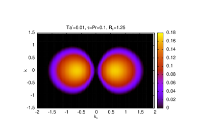
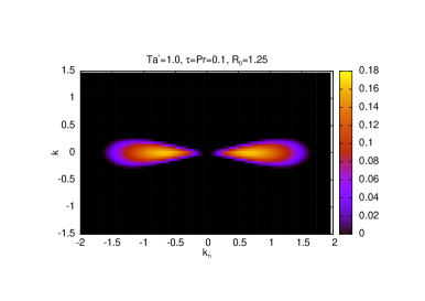
Figure 1: Variation of the real part of $\lambda$ with input wavenumbers ($k,k_{h}$) for ${\rm Ta^{*}}=0.01$ (left) and ${\rm Ta^{*}}=1$ (right) at $\tau={\rm Pr}=0.1$, $R_{0}=1.25$. In both cases, $\theta=0$. Note that, as discussed in the text, the fastest-growing modes have $k=0$.

These so called “elevator” modes are unaffected by rotation as can be seen in Fig 1 and by direct inspection of Eq (11) since the last term (containing ${\rm Ta}^{*}$) vanishes for $k=0$ and $\theta=0$. The modes with $k\neq 0$ by contrast are suppressed by rotation in the sense that the higher $k$ modes grow more slowly or become stable with increasing ${\rm Ta}^{*}$.
While linear theory helps to determine the linearly unstable regions of parameter space, quantifying mixing by fingering convection can only be done using nonlinear arguments. In the non-rotating case, Radko & Smith (2012); Brown et al. (2013) showed that the nonlinear saturation of the fingering instability is due to the shear that inevitably develops between upflowing and downflowing fingers. By matching the growth rates of the fingers to the growth rates of the emerging shear instability, they successfully predicted the amplitude of the vertical velocity at saturation which they then used to model the turbulent mixing coefficient.

Since rotation has a tendency to stabilize a system against motion perpendicular to the rotation axis, we may expect it to stabilize the fingers against the shear instabilities that cause their nonlinear saturation. In that case, the vertical velocity within the fingers might be permitted to grow to much larger amplitude before the secondary shear instabilities develop, which could in turn lead to the enhancement in the efficiency of vertical transport in rotating fingering convection compared with the non-rotating case. This intuitive picture, and its obvious potential for explaining the “missing mixing” in RGB stars, motivated us to run DNSs of rotating fingering convection. In what follows, we first attempt to estimate when the effects of rotation may become important, and then present nonlinear DNSs of rotating fingering convection to test these ideas.

4 Estimating when rotation is important in stellar interiors

While rotation does not have any effect on the growth rate of the fastest-growing fingering modes, it is very likely to have one on their nonlinear saturation (see our discussion above and the findings of Moll & Garaud (2017) for the effect of rotation on the nonlinear saturation of the ODDC instability). A commonly-used measure of the relative strength of inertial forces ($\mathbf{u}\cdot\nabla\mathbf{u}$) to Coriolis forces ($2\mathbf{\Omega}\times\mathbf{u}$) is the Rossby number, defined as

$${\rm Ro}=\frac{U}{2\Omega L},$$ (13)

where $U$ and $L$ are typical dimensional velocities and length-scales associated with the fluid motions in consideration. In turbulent flows, the effect of rotation is therefore negligible if ${\rm Ro}\gg 1$, but dominant if ${\rm Ro}\ll 1$. For moderate and high ${\rm Pr}$ fingering convection and ODDC, since $U\sim\frac{\kappa_{T}}{d}$ and $L\sim d$ (Traxler et al. (2011b); Mirouh et al. (2012); Wood et al. (2013); Moll et al. (2016)), one may estimate ${\rm Ro}$ as

$${\rm Ro}\sim\frac{\frac{\kappa_{T}}{d}}{2\Omega d}\sim\frac{1}{\sqrt{{\rm Ta}^{*}}},$$ (14)

which would imply that ${\rm Ta}^{*}\gg 1$ double-diffusive systems should be strongly rotationally constrained, while ${\rm Ta}^{*}\ll 1$ systems should not feel the effect of rotation at all. This was verified to be true for ${\rm Pr}\sim 1$ down to ${\rm Pr}\sim 0.01$ for ODDC (see Moll & Garaud (2017)), for instance.
However in stellar interiors, the Prandtl number is asymptotically small, taking values ranging from $10^{-6}$ down to $10^{-9}$. In this regime, the vertical velocities within individual fingers do not scale as above, but instead are expected to scale with Pr (Brown et al. (2013), and see below). Hence, the effective Rossby number of rotating fingering convection is predicted to be significantly different from the estimate given in (14).
Indeed, for the parameter regime appropriate for stellar interiors, $U$ and $L$ can be estimated using the results of Brown et al. (2013). They argue that

$$U\sim\frac{\lambda_{max}}{L},\ L\sim\frac{2\pi}{l_{max}},$$ (15)

where $\lambda_{max}$ is the growth rate of the fastest growing linearly unstable mode, and $l_{max}$ is the associated horizontal wavenumber.

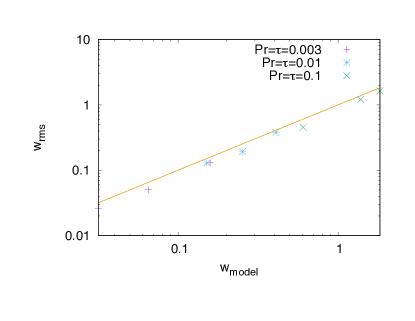
Figure 2: Comparison of the rms vertical velocities (symbols) estimated using the prediction of the Brown model (given by the line representing $w_{model}=\frac{2\pi\lambda_{max}}{l_{max}}$) with results of non-rotating DNSs from Traxler et al. (2011b); Brown et al. (2013); Garaud (2018).

We can test this scaling by comparing for instance the r.m.s. vertical velocity $w_{rms}$ extracted by reanalyzing non-rotating DNSs at moderately low values of ${\rm Pr}$ presented in Traxler et al. (2011b); Brown et al. (2013); Garaud (2018), against our theoretical prediction from (15), namely,

$$w_{model}=\frac{\lambda_{max}l_{max}}{2\pi}$$ (16)

where $\lambda_{max}$ and $l_{max}$ are found numerically by maximizing the solutions of (11) for ${\rm Ta^{*}=0}$, $k=0$ and $\theta=0$ against all possible value of $l$. This comparison is shown in Fig 2, and clearly demonstrates that $w_{model}$ is a remarkably accurate estimate for $w_{rms}$ across the entire range of Prandtl numbers and density ratios tested. This would in turn imply that the Rossby number of rotating fingering convection could, at a first approximation, be given by

$${\rm Ro}=\frac{\lambda_{max}}{2\Omega}.$$ (17)

In the asymptotic regime where ${\rm Pr},\tau\ll r\ll 1$, where $r=\frac{R_{0}-1}{\tau^{-1}-1}$ (which is the regime most appropriate for stellar interiors), Brown et al. (2013) further showed that

$$\lambda_{max}\simeq{\rm Pr}\sqrt{\frac{\tau}{r{\rm Pr}}},$$ (18)

resulting in the following predicted scaling for ${\rm Ro}$ with all the input parameters:

$${\rm Ro}\sim\sqrt{\frac{{\rm Pr}}{R_{0}-1}}\frac{1}{\sqrt{{\rm Ta}^{*}}}.$$ (19)

Since $d$ is related to the buoyancy frequency, $N$, as

$$d^{4}=\frac{\kappa_{T}\nu}{N^{2}},$$ (20)

we can write ${\rm Ta}^{*}$ (given by 8) as

$${\rm Ta}^{*}={\rm Pr}\frac{\varOmega^{2}}{N^{2}}.$$ (21)

Thus, our estimate for the Rossby number is simply given by

$${\rm Ro}\sim\sqrt{\frac{N^{2}}{\varOmega^{2}}\frac{1}{R_{0}-1}}.$$ (22)

Using a typical value of $N^{2}\sim 10^{-4}$ in the radiative zone of a solar-mass RGB star, one can estimate the Rossby number in the region just above the hydrogen-burning shell using observed estimates for red-giant rotation rates inferred from astroseismic data from Kepler (Deheuvels et al. (2014)) that range between $\sim 0.25-10$ times the solar rotation rate ($\sim 400nHz$). Assuming a rather extreme estimate for density ratio $R_{0}\sim 10^{3}$(Denissenkov (2010)), we find that the Rossby number would be in the range $0.1\lesssim{\rm Ro}\lesssim 10$ for slow rotators and $0.016\lesssim{\rm Ro}\lesssim 1.6$ for fast rotators, at the onset of fingering convection in RGB stars. This then strongly suggests that rotation must be taken into account in modeling fingering convection in these objects.
In the following section, we therefore present new DNSs of rotating fingering convection, with values of ${\rm Ro}$ spanning the anticipated range ($0.05-5$) for RGB stars.

5 Numerical simulations

5.1 Numerical tool: PADDI

We use a version of the pseudo-spectral, triply periodic PADDI code (Stellmach & Hansen (2008), Traxler et al. (2011b), Stellmach et al. (2011)) modified in Moll & Garaud (2017) to include the effects of rotation. We perform DNSs for ${\rm Ta}^{*}=0,0.01,0.1,1,10,25$ and $100$. We anticipate fingers to become taller for increasing values of $R_{0}\text{ or }{\rm Ta}^{*}$ and hence choose an elongated (rectangular) box with dimensions $100d\times 100d\times 200d$ as our default domain size. This is adjusted as and when required for varying $R_{0}$ and ${\rm Ta}^{*}$ (see Table 1). For simplicity, we only present results for a domain at the poles with the rotation axis aligned with the z-direction, i.e. $\theta=0$ in (3). In all of our simulations, the temperature and composition fields are initialized with small amplitude random noise. Since performing DNSs at realistic values of ${\rm Pr},\tau$ for stellar interiors is computationally unfeasible as of now, we can only run simulations at parameters down to ${\rm Pr}=\tau=0.01$ at best. For this exploratory work, we prefer ${\rm Pr}=\tau=0.1$, because it allows us to comprehensively explore the effects of varying $R_{0}$ and ${\rm Ta}^{*}$. We now look at a few sample simulations.

5.2 Sample runs at $Pr=\tau=0.1$

For this choice of $\tau=0.1$, a system is unstable to fingering provided $1<R_{0}<10$. We focus our study on two values of $R_{0}=1.45$ and $5$ - the former representing conditions close to being convectively unstable and the latter being half-way through the fingering-unstable range. We summarize the results of our DNSs for different choices of ${\rm Ta^{*}}$ (which varies with the Rossby number ${\rm Ro}$) and $R_{0}$ in Table 1.
Fig 3 shows snapshots of the vertical velocity field in six different simulations spanning values of ${\rm Ta}^{*}=0.01,1\,\mbox{and\,}10$ for two values of $R_{0}=1.45$ and $5$. As can be readily seen from the snapshots, at ${\rm Ta}^{*}=0.01$ (which is in the “slowly rotating” regime), the fingers become more stable with increasing stratification (i.e. increasing $R_{0}$) which has also been observed experimentally (Krishnamurti (2003)) and in DNSs of non-rotating fingering convection (Traxler et al. (2011b)). With increasing values of ${\rm Ta}^{*}$, we observe a propensity of the flow to become invariant along the axis of rotation. This is in accordance with the Taylor-Proudman theorem (Proudman (1916); Taylor (1917)), which becomes relevant when the Rossby number becomes much smaller than $1$. The Taylor-Proudman constraint is significantly more pronounced for the $R_{0}=5$ case than for the $R_{0}=1.45$ case, at fixed ${\rm Ta}^{*}$. To understand why this is the case, we note that the effective Rossby number, given by (19), is significantly higher at $R_{0}=1.45$ (${\rm Ro}=0.47$ for ${\rm Ta}^{*}=1$) than $R_{0}=5$ (${\rm Ro}=0.16$ for ${\rm Ta}^{*}=1$); hence achieving a Taylor-Proudman state at smaller $R_{0}$ requires larger values of ${\rm Ta^{*}}$.

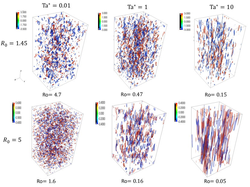
Figure 3: Snapshots of vertical velocity fields (after saturation) at ${\rm Ta}^{*}=0.01$ (top), $1$ (middle) and $10$ (bottom) for $R_{0}=1.45$ (left) and $5$ (right).

$R_{0}$	${\rm Ta}^{*}$	Resolution	$L_{x}\times L_{y}\times L_{z}$	${\rm Nu}{}_{\mu}$	$w_{rms}$	$u_{rms}$
$1.45$	$0.0$	$96\times 96\times 96$	$100\times 100\times 100$	$86.415\pm 2.378$	$1.2095\pm 0.0135$	$1.5615\pm 0.0169$
	$0.01$	$64\times 64\times 128$	$100\times 100\times 200$	$83.395\pm 1.196$	$1.187\pm 0.0006$	$1.544\pm 0.006$
	$0.1$	$64\times 64\times 128$	$100\times 100\times 200$	$75.497\pm 0.468$	$1.1406\pm 0.0039$	$1.5304\pm 0.0045$
	$1$	$64\times 64\times 128$	$100\times 100\times 200$	$62.403\pm 0.857$	$1.058\pm 0.006$	$1.482\pm 0.008$
		$128\times 128\times 256$	$100\times 100\times 200$	$61.644\pm 1.843$	$1.0507\pm 0.0158$	$1.476\pm 0.021$
	$10$	$64\times 64\times 128$	$100\times 100\times 200$	$1899.28\pm 158.055$	$2.209\pm 0.005$	$7.31\pm 0.16$
		$128\times 128\times 256$	$100\times 100\times 200$	$44.186\pm 1.49$	$0.9012\pm 0.0128$	$1.495\pm 0.048$
	$25$	$64\times 64\times 128$	$100\times 100\times 200$	$53.26\pm 3.294$	$0.984\pm 0.034$	$1.5859\pm 0.0298$
	$100$	$64\times 64\times 128$	$100\times 100\times 200$	$57.65\pm 4.07$	$1.028\pm 0.047$	$1.7358\pm 0.0431$
$5.0$	$0.0$	$128\times 128\times 128$	$100\times 100\times 100$	$11.396\pm 0.109$	$0.2575\pm 0.0019$	$0.306\pm 0.002$
	$0.01$	$64\times 64\times 128$	$100\times 100\times 200$	$9.838\pm 0.1545$	$0.23704\pm 0.0022$	$0.2929\pm 0.0022$
	$1$	$32\times 32\times 64$	$100\times 100\times 200$	$4.649\pm 0.137$	$0.1492\pm 0.0029$	$0.2355\pm 0.0039$
		$64\times 64\times 128$	$100\times 100\times 400$	$4.681\pm 0.152$	$0.1496\pm 0.0033$	$0.2397\pm 0.0041$
	$10$	$64\times 64\times 128$	$100\times 100\times 200$	$4.986\pm 0.260$	$0.1535\pm 0.0049$	$0.2277\pm 0.0036$
		$64\times 64\times 128$	$100\times 100\times 400$	$4.8046\pm 0.3054$	$0.1494\pm 0.0056$	$0.256\pm 0.008$
	$100$	$64\times 64\times 128$	$100\times 100\times 200$	$6.112\pm 0.301$	$0.167\pm 0.005$	$0.193\pm 0.006$
$9.1$	$0.0$	$32\times 32\times 64$	$100\times 100\times 200$	$1.3812\pm 0.0142$	$0.02989\pm 0.0006$	$0.0338\pm 0.0006$
	$0.01$	$64\times 64\times 128$	$100\times 100\times 200$	$1.0254\pm 0.0013$	$0.0073\pm 0.0002$	$0.0122\pm 0.0004$
	$0.1$	$32\times 32\times 64$	$100\times 100\times 200$	$1.016\pm 0.001$	$0.0057\pm 0.0002$	$0.01025\pm 0.00029$
	$1$	$32\times 32\times 64$	$100\times 100\times 200$	$1.0267\pm 0.0045$	$0.0069\pm 0.0006$	$0.0107\pm 0.0011$
		$32\times 32\times 64$	$100\times 100\times 800$	$1.0153\pm 0.0011$	$0.0056\pm 0.0002$	$0.01003\pm 0.0003$
	$10$	$32\times 32\times 64$	$100\times 100\times 200$	$1.248\pm 0.018$	$0.0207\pm 0.0008$	$0.02366\pm 0.00095$
		$32\times 32\times 128$	$100\times 100\times 1600$	$1.01376\pm 0.00089$	$0.0055\pm 0.0002$	$0.00964\pm 0.0003$
	$25$	$32\times 32\times 64$	$100\times 100\times 200$	$1.601\pm 0.027$	$0.032\pm 0.001$	$0.034\pm 0.001$
		$32\times 32\times 64$	$100\times 100\times 800$	$1.039\pm 0.005$	$0.00831\pm 0.0006$	$0.01229\pm 0.00099$

Table 1: DNS runs for chosen set of parameters ${\rm Ta}^{*}\mbox{ and }R_{0}$ at ${\rm Pr}=\tau=0.1$

Using the set of rotating DNSs, we can actually compare our theoretical estimate for the Rossby number ${\rm Ro}$ (see (19)), to the effective Rossby number of the simulations which is given by

$${\rm Ro}_{f}\sim\frac{w_{rms}}{10\sqrt{{\rm Ta}^{*}}},$$ (23)

where $w_{rms}$ is the measured rms vertical velocity in the DNS, and the number $10$ comes from assuming that the horizontal dimensions of the fingers are of the order of $10d$ (which roughly corresponds to the width of the fastest-growing fingers). The results are shown in Fig 4 and confirm that the predicted ${\rm Ro}$ derived in Section 4 is a fairly good estimate of the effective Rossby number of the fingers (${\rm Ro}_{f}$) in all of our rotating simulations.

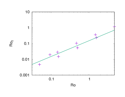
Figure 4: Comparison of the predicted Rossby number, ${\rm Ro}$ (given by 19) with the effective Rossby number of the fingers, ${\rm Ro}_{f}$, measured from the DNSs according to (23).

Finally, note that as in Traxler (2011), the elongation of the fingers along the vertical direction (either for high $R_{0}$, or high ${\rm Ta^{*}}$, or both) poses a numerical challenge. Indeed, we need to ensure that our domain is large enough so that the fingers do not “feel” its boundaries, which would lead to artificial enhancements of the transport rates due to the assumption of periodic boundary conditions. This problem is discussed in more detail in Appendix.

5.3 Effect of rotation on compositional transport by small-scale fingering convection

In what follows, we now only report on the simulations with the largest resolution and domain sizes available at $R_{0}=1.45$ and $5$. We measure the vertical flux of composition in terms of the compositional Nusselt number, ${\rm Nu_{\mu}}$ defined as:

$${\rm Nu_{\mu}}=1-\frac{R_{0}}{\tau}\langle\tilde{w}\tilde{\mu}\rangle,$$ (24)

where $\left\langle\right\rangle$ denotes a volume average over the entire domain. ${\rm Nu}_{\mu}$ can be interpreted as the ratio of the effective diffusivity $D_{\mu}$ to the microscopic diffusivity $\kappa_{\mu}$ i.e.

$$D_{\mu}=\kappa_{\mu}{\rm Nu_{\mu}.}$$ (25)

As usual, the turbulent transport of heat is negligible in fingering convection. The time-evolution of ${\rm Nu_{\mu}}$ is shown in Figure 5 for different values of ${\rm Ta}^{*}$. As expected, we see the development of the fingering instability at early times, followed by its nonlinear saturation. As anticipated from our naive argument of Section 3, we find that the peak compositional transport increases significantly with ${\rm Ta}{}^{*}$, suggesting that the shear instability between the fingers is indeed stabilized by rotation. However, we also see that the turbulent transport rates after saturation of the fingering instability, once the system has achieved a statistically steady state, do not depend on ${\rm Ta}{}^{*}$ nearly as much. To see this more quantitatively, we measure the transport properties of fingering convection in that statistically stationary state.

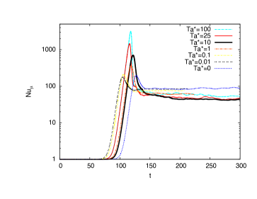
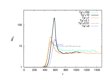
Figure 5: ${\rm Nu}{}_{\mu}$ as function of time (in units of diffusion time scale) for simulations with ${\rm Pr}=\tau=0.1$ , and varying ${\rm Ta}^{*}$ at $R_{0}=1.45$ (left) and $5$ (right).

The time-averaged ${\rm Nu}{}_{\mu}$ values thus extracted for different values of ${\rm Ta}^{*}$ are presented in Figure 6 for both values of $R_{0}$, as a function of the corresponding Rossby numbers, ${\rm Ro}$ (as given by Eq 19). This shows that rotation actually tends to lower the vertical transport rates by a factor of up to 2 compared with the non-rotating case.

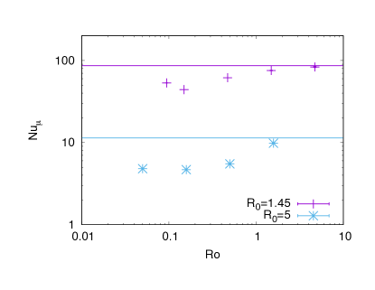
Figure 6: Time-averaged ${\rm Nu}{}_{\mu}$ in the statistically steady state as a function of the estimated Rossby number ${\rm Ro}$ at $R_{0}=1.45$ and $5$ - the horizontal lines shows the corresponding non-rotating (${\rm Ro}\rightarrow\infty$) ${\rm Nu}{}_{\mu}$ values.

This is a rather unexpected finding in light of our discussions in Section 3 where we expected that rotation would act to enhance the r.m.s. vertical velocities and therefore also the mixing rates. Instead, we find that both vertical and horizontal r.m.s. velocities remains almost unchanged as the rotation rate is increased (see Fig 7).

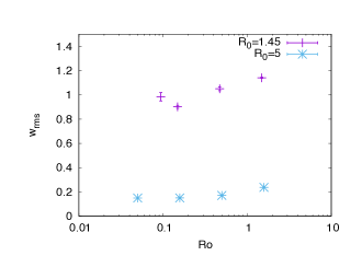
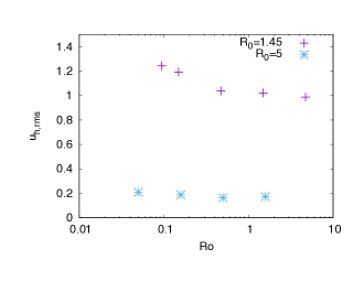
Figure 7: The rms vertical ($w_{rms}$) and total horizontal ($u_{h,rms}=\sqrt{u_{rms}^{2}+v_{rms}^{2}}$) velocities as a function of the Rossby number ${\rm Ro}$ for DNSs at $R_{0}=1.45$ and 5.

5.4 Emergence of a large scale vortex

While all the results reported so far were from high-resolution simulations, we ran a few additional simulation at half their resolution for much longer to see if any longer-term dynamics emerge. These runs are not particularly under-resolved, so their dynamics are still reliable i.e. the fingers and their structure are still well resolved. Interestingly, one such run at a resolution of $64\times 64\times 128$ for $R_{0}=1.45$ and ${\rm Ta}^{*}=10$ shows a significant enhancement in ${\rm Nu}{}_{\mu}$ over a long timescale ($\sim 3000$ time units), as shown in the left panel of Fig 8.

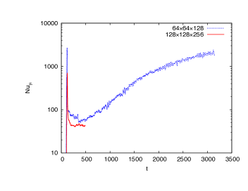
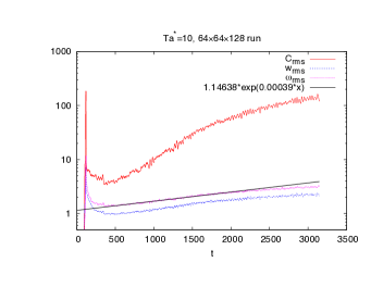
Figure 8: (left) Enhancement in chemical transport rates, measured in terms of ${\rm Nu}_{\mu}$ observed at $R_{0}=1.45$ and ${\rm Ta}^{*}=10$ for $64\times 64\times 128$ run compared to a $128\times 128\times 256$ run; (right) growth in rms values of the chemical field and vertical components of velocity and vorticity in the $64\times 64\times 128$ run.

It also shows a steady increase in the rms values of the vertical velocity, chemical field ($\mu_{rms}$) as well as the vertical component of the vorticity field, $\omega_{rms}$ (see right panel of Fig 8). Fig 9 shows horizontal ($x-y$ plane) snapshots of the vertical velocity and the chemical fields at time $t=1300$, and reveals the presence of a cyclonic large scale vortex (hereafter, referred to as LSV). The LSV shows a substantial enhancement in the concentration of high-$\mu$ fluid at its core, associated with a strengthening of the downward vertical component of velocity. It is to be noted that LSVs seen in other simulations can also have the reverse situation, with low-$\mu$ material in their core flowing upward. In both cases,

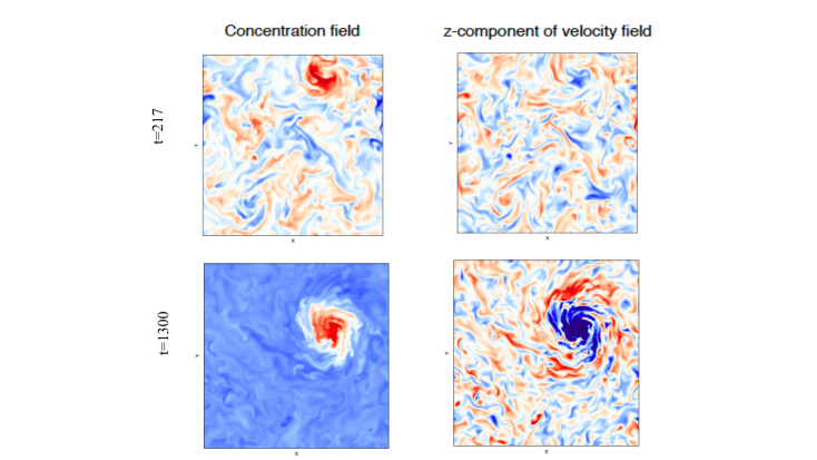
Figure 9: Horizontal snapshots of chemical (left) and vertical velocity (right) fields at $t=217$ (top) and $t=1300$ (bottom) for the $64\times 64\times 128$ run at $R_{0}=1.45,\,{\rm Ta}^{*}=10$ - red shows positive and blue shows negative values of the quantities.

this causes the enhancement in chemical transport measured through the increase in ${\rm Nu}_{\mu}$ in Fig 8. Fig 10 presents volume rendered snapshots of the vertical vorticity in the flow at time $t=217$ and $t=1300$, and clearly shows the emergence of long coherent cyclonic vortices that later merge into a single cyclonic LSV spanning the entire height and width of our domain.
In order to understand why this vortex forms and grows to fill the domain, we inspect the horizontal energy spectrum of the simulation (shown in left panel of Fig 11) which clearly shows the development over time of a well-defined power law at low horizontal wavenumber $k_{h}$, which is typical of an inverse energy cascade associated with rotation. The inverse cascade draws its energy at the injection scale $k_{h}\sim 0.5$, which corresponds to the typical wavenumber of the fastest-growing fingering modes. We can also estimate the rate at which the LSV grows in strength by fitting an exponential to the vorticity, $\omega_{rms}$ (between $t\sim 500-2000)$ as shown in the right panel of Fig 8, which gives a value of $\sim 0.00039$ per unit time. The corresponding growth timescale, which would be of order $3000$, is much larger than an eddy turnover timescale (which is of order $10$), but much smaller than the thermal or viscous diffusion timescales across the domain (which are of order $10^{4}$ and $10^{5}$ respectively).

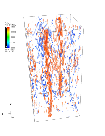
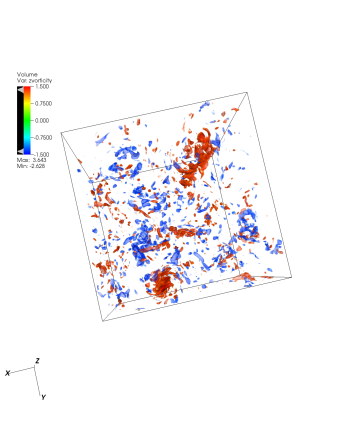
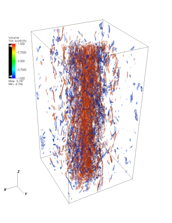
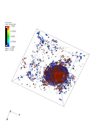
Figure 10: (left) Snapshots of vertical vorticity $\omega_{z}=\left(\nabla\times\mathbf{u}\right)_{z}$; (right) top view (along $x-y$ plane) - upper panels show two cyclonic vortices at $t=217$ that later merge into a LSV shown in the bottom two panels at $t=1300$.

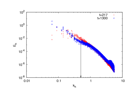
Figure 11: Evolution of the horizontal energy, $E_{h}=\frac{1}{2}(u^{2}+v^{2})$, for the lower resolution run (see text for details) at $R_{0}=1.45$ and ${\rm Ta}^{*}=10$, showing the gradual growth in energy of low $k_{h}=\sqrt{l^{2}+m{}^{2}}$ modes with time, and the presence of an inverse energy cascade; the arrow head shows the position of the energy injection scale ($k_{h}\sim 0.5$) corresponding to the typical wavenumber of the fastest growing fingering modes.

The emergence of such LSVs is reminiscent of similar findings in the work by Moll & Garaud (2017) (for the ODDC case) as well as in studies of rapidly rotating convection (Guervilly et al. (2014)). In all such cases, LSVs are always seen to fill the domain, and have also been interpreted as resulting from an inverse cascade (Julien et al. (2018)).

6 Discussion

6.1 Summary of our findings

We have investigated the effect of rotation on the linear growth of the fingering instability (Section 3) and found that rotation does not affect the growth rate of the fastest-growing modes of the basic linear instability. It does however influence its nonlinear evolution and saturation. With the help of DNSs (Section 5) using the PADDI code, we have measured the compositional transport rates of rotating fingering convection in a parameter regime that approaches stellar conditions. In general, we have found that rotation does not enhance mixing by fingering convection contrary to our original expectations. In fact, rotation seems to have a mild stabilizing effect on mixing. The compositional transport rates predicted across a wide range of rotation rates are consistently lower than the corresponding non-rotating values measured in previous DNSs (Denissenkov (2010),Traxler et al. (2011b); Brown et al. (2013)). For simplicity, we restricted our present study to the polar configuration only, so these findings need to be verified for the non-polar cases. We suspect, however, that non-polar configurations will have even weaker vertical mixing rates, simply by virtue of their geometry.

We have observed a possible exception to this general finding for a particularly turbulent (low $R_{0}$) and rapidly rotating (low ${\rm Ro}$) run in which coherent large scale structures naturally emerge and gradually evolve to merge into a single cyclonic large scale vortex spanning the entire computation domain. This LSV causes a significant enhancement in the compositional transport rates by concentrating high-$\mu$ material at its core that is advected downward. Inspection of the horizontal kinetic energy spectrum demonstrates that the LSV forms through a rotationally-driven inverse cascade that draws its energy from the basic instability at the finger scale. The LSV formation and dynamics are strongly reminiscent of those observed in a variety of other rapidly rotating turbulent systems, such as convection (Guervilly et al. (2014); Julien et al. (2018)), stratified turbulence (Marino et al. (2013); Oks et al. (2017)) and oscillatory double-diffusive convection (Moll & Garaud (2017)).

6.2 Implications for mixing in stars

Our findings raise a tantalizing possibility: if these large-scale vortices (LSVs) also form in the fingering regions of RGB stars, they could substantially enhance the efficiency of mixing by fingering convection, and thereby provide a self-consistent scenario to explain the observed abundance changes on the upper RGB (Gratton et al. (2000); Charbonnel & Zahn (2007b)). This raises the obvious question of whether LSVs would form under more realistic stellar conditions. Studies of rapidly rotating convection and oscillatory double-diffusive convection in the polar configuration (i.e. with rotation aligned with gravity) have generally concluded that LSVs are only observed in a rotationally constrained (low Rossby number) and yet also strongly turbulent (high Reynolds number) regime (Guervilly et al. (2014); Julien et al. (2018); Seshasayanan & Alexakis (2018)), which is also what we found here. The first of these conditions can be understood by noting that strong rotation is required to trigger an inverse energy cascade. However, rotation cannot be too strong otherwise the flow becomes vertically invariant (through the Taylor-Proudman constraint) and horizontal motions can only decay in that case. To see this, note that the vertical component of the vorticity equation (obtained by taking the curl of 4) reduces to

$$\frac{\partial\omega_{z}}{\partial t}+\mathbf{u}\cdot\nabla\omega_{z}={\rm Pr}\nabla^{2}\omega_{z}$$ (26)

when motions are independent of $z$. In that limit, $\omega_{z}$ must ultimately decay with time (since this advection-diffusion equation contains no source term), which in turn shows that horizontal motions must necessarily decay as well. In other words, the flow must remain sufficiently three-dimensional to continually feed energy into the inverse cascade and maintain the vortex against viscous decay, hence the need for a sufficiently large Reynolds number.

In Section 4 (combined with the results of Figure 4), we showed that the fingering regions of RGB stars would indeed satisfy the low Rossby number requirement, with estimated values in the range $10^{-3}-1$ for rapid and moderate rotators. To estimate the Reynolds number ${\rm Re}$ expected in these regions, we use a similar argument as in Section 4. Since ${\rm Re}=UL/\nu$, where $U$ and $L$ are the characteristic velocities and lengthscale of fingering flows (given by equation 15) and $\nu$ is the viscosity, then

$${\rm Re\simeq\sqrt{\frac{\tau}{r{\rm Pr}}}}\simeq\frac{1}{\sqrt{{\rm Pr}(R_{0}-1)}}.$$ (27)

According to this estimate, using ${\rm Pr}\sim 10^{-6}$ and $R_{0}\sim 10^{3}$, as before, we find that ${\rm Re}\sim 10^{2}$, which should indeed be sufficiently high for LSVs to form.

We therefore conclude that fingering regions of RGB stars can indeed potentially be the home of large-scale vortices near the poles, which would cause a very substantial enhancement of the compositional fluxes and could in turn explain the observed evolution of the surface abundances after the luminosity bump.

Of course, much remains to be done to confirm this scenario. In particular, recent results on the formation of large-scale vortices in other systems such as rotating convection and oscillatory double-diffusive convection suggest that they may not develop (1) at lower latitudes (Moll & Garaud (2017)), and (2) unless the computational domain has a unit aspect ratio (Julien et al. (2018)). In these cases, large-scale horizontal jets form instead. Whether these would also be more common in the case of rotating fingering convection remains to be determined, but is likely. Whether compositional transport would similarly be enhanced in the presence of jets or not also remains to be determined, but also seems likely. These questions will be answered in future work, as they require substantial computational resources to fully explore.

7 Conclusions

The simulations presented here clearly point out the need to understand better the interplay of different physical mechanisms in order to provide robust estimates of mixing to be used in stellar evolutionary calculations. Most modern stellar evolution codes treat mixing processes independently, by computing a simple diffusion coefficient for each one of them and then adding them together (Cantiello & Langer (2010); Lagarde et al. (2011); Matrozis & Stancliffe (2017); Paxton et al. (2018)). This study reveals that although rotation and fingering convection can indeed be fairly well understood independently in some regimes, other regimes exist in which they strongly reinforce one another. We showed that this regime is precisely the one that is relevant for the RGB “extra-mixing” problem. If indeed LSVs form in the radiative zone above the H-burning shell in the interiors of RGB stars, they could greatly enhance transport and provide a self-consistent scenario explaining the observed abundances changes on the upper RGB which non-rotating model predictions fail to do. This is the only possible scenario in the context of the “missing-mixing” problem of the RGBs which could work to explain the observed change in abundances of red-giants above the luminosity bump in a self-consistent way without the need to invoke physical mechanisms that are not specific to this particular evolutionary phase (Charbonnel & Zahn (2007a); Denissenkov et al. (2009)).We aim to explore the emergence of these LSVs across a wider range of parameter space in a future work (Sengupta & Garaud, in preparation) to make more systematic predictions for the conditions in which one can expect them to form.

Appendix

Effect of domain size

From Table 1, we can note that for $R_{0}=5$, the difference in the compositional Nusselt numbers between two simulations for which the height of the domain differs by factor of $2,$ is at most few percent even for our highest ${\rm Ta}^{*}$ runs. However, for a more extreme choice of $R_{0}=9.1$, Fig 12 shows that using our default domain size at ${\rm Ta}^{*}=10$ or $25$ gives compositional fluxes that differ by up to an order of magnitude from those obtained by using a taller domain ($100d\times 100d\times 800d$). A similar effect was also observed by Traxler (2011) even for the non-rotating case for very high values of $R_{0}$ close to the marginal stability threshold of $\frac{1}{\tau}$.

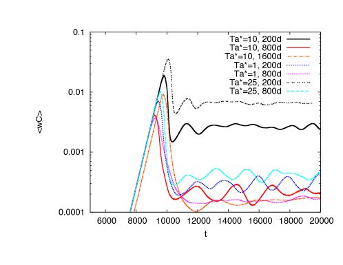
Figure 12: Compositional fluxes for simulations using domain heights of $200d$ and $800d$ at $R_{0}=9.1$ for ${\rm Ta}^{*}=1.0,10.0$

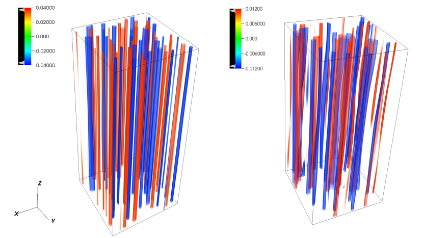
Figure 13: Vertical velocity fields (after saturation) for $R_{0}=9.1$ and ${\rm Ta}^{*}=10$ for domain heights of $200d$(left) and $800d$ (right), showing the need for using an elongated domain (in the vertical direction) at high $R_{0}$.

Fig 13 shows snapshots of the vertical velocity in two simulations for $R_{0}=9.1$, ${\rm Ta}^{*}=10$ - the left panel using our default domain size and the right panel with a $100d\times 100d\times 800d$ domain. The $200d$-tall domain has fingers that are perfectly vertical, whereas the $800d$-tall domain, shows fingers that no longer remain perfectly vertical. We conjecture that the fastest growing wavelength of the shear instability between upflowing and downflowing fingers increases with increasing rotation rate. When the latter exceeds the domain size, the shear instability is suppressed and the transport is vastly enhanced. This effect is artificial, however, and must be avoided by making sure the domain is indeed tall enough to contain the shear-unstable modes.

References

- Boussinesq (1903) Boussinesq, J. 1903, Théorie analytique de la chaleur: mise en harmonie avec la thermodynamique et avec la théorie mécanique de la lumière, Vol. 2 (Gauthier-Villars)
- Brown et al. (2013) Brown, J. M., Garaud, P., & Stellmach, S. 2013, ApJ, 768, 34
- Cantiello & Langer (2010) Cantiello, M., & Langer, N. 2010, A&A, 521, A9
- Charbonnel & Zahn (2007a) Charbonnel, C., & Zahn, J.-P. 2007a, A&A, 476, L29
- Charbonnel & Zahn (2007b) —. 2007b, A&A, 467, L15
- Deal et al. (2013) Deal, M., Deheuvels, S., Vauclair, G., Vauclair, S., & Wachlin, F. C. 2013, A&A, 557, L12
- Deheuvels et al. (2014) Deheuvels, S., et al. 2014, A&A, 564, A27
- Denissenkov (2010) Denissenkov, P. A. 2010, ApJ, 723, 563
- Denissenkov et al. (2013) Denissenkov, P. A., Herwig, F., Bildsten, L., & Paxton, B. 2013, ApJ, 762, 8
- Denissenkov & Merryfield (2011) Denissenkov, P. A., & Merryfield, W. J. 2011, ApJ, 727, L8
- Denissenkov & Pinsonneault (2008) Denissenkov, P. A., & Pinsonneault, M. 2008, ApJ, 684, 626
- Denissenkov et al. (2009) Denissenkov, P. A., Pinsonneault, M., & MacGregor, K. B. 2009, ApJ, 696, 1823
- Garaud (2011) Garaud, P. 2011, ApJ, 728, L30
- Garaud (2018) —. 2018, Annual Review of Fluid Mechanics, 50, 275
- Garaud et al. (2015) Garaud, P., Medrano, M., Brown, J. M., Mankovich, C., & Moore, K. 2015, ApJ, 808, 89
- Gratton et al. (2000) Gratton, R. G., Sneden, C., Carretta, E., & Bragaglia, A. 2000, A&A, 354, 169
- Guervilly et al. (2014) Guervilly, C., Hughes, D. W., & Jones, C. A. 2014, Journal of Fluid Mechanics, 758, 407
- Julien et al. (2018) Julien, K., Knobloch, E., & Plumley, M. 2018, Journal of Fluid Mechanics, 837, R4
- Krishnamurti (2003) Krishnamurti, R. 2003, Journal of Fluid Mechanics, 483, 287
- Lagarde et al. (2011) Lagarde, N., Charbonnel, C., Decressin, T., & Hagelberg, J. 2011, A&A, 536, A28
- Leconte (2018) Leconte, J. 2018, ApJ, 853, L30
- Marino et al. (2013) Marino, R., Mininni, P. D., Rosenberg, D., & Pouquet, A. 2013, EPL (Europhysics Letters), 102, 44006
- Marks & Sarna (1998) Marks, P. B., & Sarna, M. J. 1998, MNRAS, 301, 699
- Marks et al. (1997) Marks, P. B., Sarna, M. J., & Prialnik, D. 1997, MNRAS, 290, 283
- Matrozis & Stancliffe (2017) Matrozis, E., & Stancliffe, R. J. 2017, A&A, 606, A55
- Medrano et al. (2014) Medrano, M., Garaud, P., & Stellmach, S. 2014, ApJ, 792, L30
- Mirouh et al. (2012) Mirouh, G. M., Garaud, P., Stellmach, S., Traxler, A. L., & Wood, T. S. 2012, ApJ, 750, 61
- Moll & Garaud (2017) Moll, R., & Garaud, P. 2017, ApJ, 834, 44
- Moll et al. (2016) Moll, R., Garaud, P., & Stellmach, S. 2016, ApJ, 823, 33
- Oks et al. (2017) Oks, D., Mininni, P. D., Marino, R., & Pouquet, A. 2017, Physics of Fluids, 29, 111109
- Paxton et al. (2018) Paxton, B., et al. 2018, ApJS, 234, 34
- Proudman (1916) Proudman, J. 1916, Proceedings of the Royal Society of London Series A, 92, 408
- Radko & Smith (2012) Radko, T., & Smith, D. P. 2012, Journal of Fluid Mechanics, 692, 5
- Seshasayanan & Alexakis (2018) Seshasayanan, K., & Alexakis, A. 2018, Journal of Fluid Mechanics, 841, 434?462
- Spiegel & Veronis (1960) Spiegel, E. A., & Veronis, G. 1960, ApJ, 131, 442
- Stancliffe et al. (2007) Stancliffe, R. J., Glebbeek, E., Izzard, R. G., & Pols, O. R. 2007, A&A, 464, L57
- Stellmach & Hansen (2008) Stellmach, S., & Hansen, U. 2008, Geochemistry, Geophysics, Geosystems, 9, Q05003
- Stellmach et al. (2011) Stellmach, S., Traxler, A., Garaud, P., Brummell, N., & Radko, T. 2011, Journal of Fluid Mechanics, 677, 554
- Taylor (1917) Taylor, G. I. 1917, Proceedings of the Royal Society of London Series A, 93, 99
- Theado & Vauclair (2010) Theado, S., & Vauclair, S. 2010, Ap&SS, 328, 209
- Traxler et al. (2011a) Traxler, A., Garaud, P., & Stellmach, S. 2011a, ApJ, 728, L29
- Traxler et al. (2011b) Traxler, A., Stellmach, S., Garaud, P., Radko, T., & Brummell, N. 2011b, Journal of Fluid Mechanics, 677, 530
- Traxler (2011) Traxler, A. L. 2011, PhD thesis, University of California, Santa Cruz
- Tremblin et al. (2016) Tremblin, P., Amundsen, D. S., Chabrier, G., Baraffe, I., Drummond, B., Hinkley, S., Mourier, P., & Venot, O. 2016, ApJ, 817, L19
- Tremblin et al. (2015) Tremblin, P., Amundsen, D. S., Mourier, P., Baraffe, I., Chabrier, G., Drummond, B., Homeier, D., & Venot, O. 2015, ApJ, 804, L17
- Vauclair (2004) Vauclair, S. 2004, ApJ, 605, 874
- Vauclair & Théado (2012) Vauclair, S., & Théado, S. 2012, ApJ, 753, 49
- Wachlin et al. (2014) Wachlin, F. C., Vauclair, S., & Althaus, L. G. 2014, A&A, 570, A58
- Wood et al. (2013) Wood, T. S., Garaud, P., & Stellmach, S. 2013, ApJ, 768, 157