A Likelihood Ratio Approach for Precise Discovery

of Truly Relevant Protein Markers

Lin-Yang Cheng,   Bowei Xi

Department of Statistics, Purdue University

Corresponding to: Bowei Xi, Department of Statistics, Purdue University,

West Lafayette, IN, 47907. xbw@purdue.edu

Abstract: The process of biomarker discovery is typically lengthy and costly, involving the phases of discovery, qualification, verification, and validation before clinical evaluation. Being able to efficiently identify the truly relevant markers in discovery studies can significantly simplify the process. However, in discovery studies the sample size is typically small while the number of markers being explored is much larger. Hence discovery studies suffer from sparsity and high dimensionality issues. Currently the state-of-the-art methods either find too many false positives or fail to identify many truly relevant markers. In this paper we develop a likelihood ratio-based approach and aim for accurately finding the truly relevant protein markers in discovery studies. Our method fits especially well with discovery studies because they are mostly balanced design due to the fact that experiments are limited and controlled. Our approach is based on the observation that the underlying distributions of expression profiles are unimodal for those irrelevant plain markers. Our method has asymptotic chi-square null distribution which facilitates the efficient control of false discovery rate. We then evaluate our method using both simulated and real experimental data. In all the experiments our method is highly effective to discover the set of truly relevant markers, leading to accurate biomarker identifications with high sensitivity and low empirical false discovery rate.

Keyword: Biomarker Discovery, Likelihood Ratio, False Discovery Rate

1 Introduction

Discovering potential protein biomarkers with clinical values is regularly a long, costly, and challenging process [Rifai et al., 2006]. Each phase of the study (i.e., discovery, qualification, verification, and validation) costs substantial amount of time and resources. In this paper we develop a statistical method to expedite the process. We aim for accurately identifying the truly relevant markers at the discovery phase, which can be directly entered for verification or even validation phrase. Figure 1 illustrates our objective.

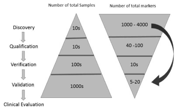
Figure 1: The typical process of biomarker discovery.

Here we focus on proteomics studies. Because following a large number of genomics studies, scientists realized that there is not necessarily high correlation between genes and proteins profiles, which implies that proteomics provides important complementary information to genomics [Pandey et al., 2000]. Moreover, since most of the drugs are directed to interact with proteins, the protein markers are as informative as gene markers.

In proteomics, mass spectrometry is considered the most productive and reliable technique for protein quantification. In particular, data-independent acquisition (DIA) [Carvalho et al., 2010, Gillet et al., 2012] has been proven to produce high quality and reproducible throughput. Hence DIA is a very effective technique for protein quantification in discovery studies. Currently there are a number of established univariate and multivariate methods being applied to identify potential biomarkers in mass spectrometry proteomics.

LIMMA [Smyth, 2004], SAM [Tusher et al., 2001], and Rank Products [Breitling et al., 2004] are popular univariate methods. LIMMA fits linear models to each marker, then applies empirical Bayes method to form moderated t-statistics. The moderated t-statistics are used to rank and select the markers. SAM assigns a score to each marker based its “relative difference”. Markers with scores larger than a threshold value is selected. Rank Products is a non-parametric approach, based on ranks of fold changes. Markers with the smallest values are selected. Meanwhile Principal Component Analysis (PCA), Penalized Logistic Regression (PLR), Partial Least Square-Discriminant Analysis (PLS-DA), and Support Vector Machine (SVM) are well-known multivariate methods regularly used in this field as well.

In discovery studies the sample size is small while the number of markers explored is large, owing to the high throughput of DIA. Nowadays there are typically thousands of protein markers quantified by DIA experiments, out of which usually only 10-50 markers are truly relevant. Discovery studies encounter sparsity and high dimensionality issues. The above univariate methods are not effective since they often identify too many false positives due to sparsity issue, leading to an unacceptable high empirical false discovery rate (FDR). For example this is observed in multiple testing procedure. On the other hand the multivariate methods mentioned above are not effective either because of high dimensionality issue. They often identify too few of the truly relevant markers, leading to an unacceptable low sensitivity. The multivariate methods mentioned above have powerful model structures. Because they only need a small number of markers to achieve high classification accuracy, these methods stop identifying more relevant markers once they reach sufficiently accurate classification results. High FDR results in considerable waste of time and resource at the subsequent phases, while low sensitivity leads to many unidentified useful biomarkers. Therefore, there is a genuine need of a novel statistical method capable of accurately identifying the correct set of truly relevant protein markers at the discovery phase.

Here we develop a likelihood ratio based approach. In this paper, we consider the scenario where are two conditions, such as disease vs. normal. Since experiments at the initial discovery phase are mostly controlled, our method focuses on data from balanced design given two conditions. Two discriminant statistics are developed based on the likelihood ratio idea. One is for the sample size greater or equal to five per condition. The other one is for very small sample size, less than 5 per condition. The main idea behind our likelihood ratio approach is that the expression profiles for the irrelevant plain markers follow unimodal distributions, where those for the truly relevant markers follow bimodal distributions. The discriminant statistics are the likelihood ratios of a bimodal distribution versus a unimodal distribution, calculated for every protein. For larger sample size, the bimodal distribution is approximated by a mixture of normals, and the unimodal distribution is approximated by a univariate normal. For very small sample size, we use kernel method to estimate the distribution of the expression profiles, then compute the ratio of the kernel estimate versus a univariate normal. Our likelihood ratio statistics have large values for the truly relevant markers, and small values for the plain markers. Our proposed method is robust to deviations from normality as long as the null expression profiles are unimodal, even though the likelihood of normal distribution is used. Notice with the multiple t-tests, the null and alternative hypotheses compare the means of two conditions. If the null hypothesis is rejected, the two conditions have different mean values. Essentially this indicates that marker does not follow a unimodal distribution. Our approach goes beyond simply considering the mean values. We explicitly estimate or approximate the likelihood functions under the null and alternative hypotheses. Hence our approach achieves a much more accurate result.

We compare our method with the aforementioned univariate and multivariate methods for mass spectrometry-based proteomics studies. Evaluations are performed with experimental datasets where truly relevant markers are known from controlled mixtures or previous literature, as well as simulated datasets. The paper is organized as follows. Section 2 describe our likelihood ratio based approach for precise protein biomarker discovery. Section 3 shows the experimental results for our approach compared with other methods. Section 4 concludes the paper.

2 A Likelihood Ratio Approach

In this paper we develop two discriminant statistics which accurately differentiate the true markers from the plain markers. We first examine the distributions of expression profiles of plain markers, as shown in Figure 2. These are proteins from HRM data, discussed in Section 3. Plain protein markers from other experimental datasets generally share this property, i.e., their expression profiles follow unimodal distributions. We also examine the distributions of expression profiles of the truly relevant markers, as shown in Figure 3. These are also proteins from HRM data. True protein markers from other experimental datasets generally follow a bimodal distribution too, given there are two conditions.

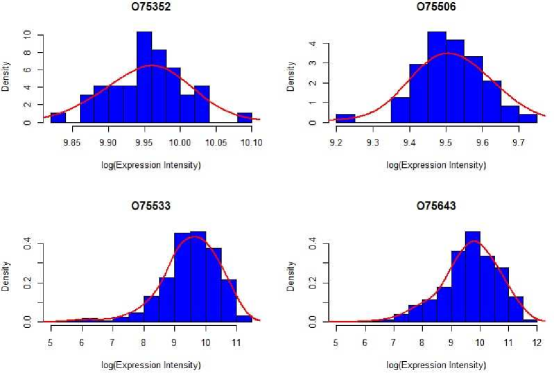
Figure 2: The expression distributions for four plain markers in HRM data.

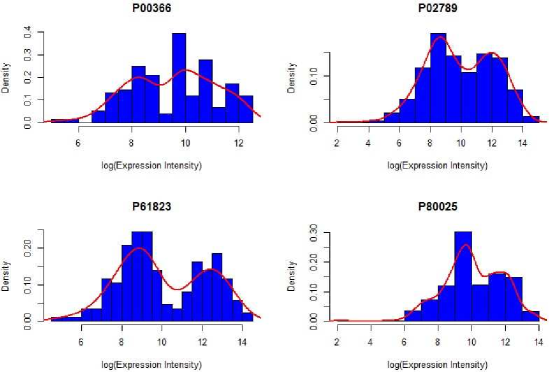
Figure 3: The expression distributions for four true markers in HRM data.

We discover that the distributions of expression profiles are usually unimodal for plain markers, and bimodal for truly relevant markers. In addition, we observe that the distributions of expression profile for truly relevant markers can be approximated by a mixtures of normals, whereas for plain markers it can be approximated by a univariate normal, given enough sample size to estimate the normal parameters. Without enough sample size, we apply kernel method to estimate the bimodal density.

2.1 A Discriminant Statistic for $n_{i}\geq 5$

Let $n_{1}$ and $n_{2}$ be the sample size for each condition, and $N=n_{1}+n_{2}$ be the total sample size. The mixture proportions of the two conditions are the sample proportions, $n_{i}/N$. We develop a likelihood ratio based discriminant statistic for larger sample size, where $n_{i}\geq 5$, $i=1,2$. It is the ratio of a mixture of normals’ density versus a univariate normal density. With relatively larger sample sizes, we approximate the bimodal distribution using a mixture of normals, and the unimodal distribution using a univariate normal. The likelihood ratio clearly differentiates the true markers from the plain markers.

Table 1: Data Layout and Notation for Condition $i$, $i=1,2$

	Protein 1	…	Protein p
Sample 1	$x^{i}_{11}$	…	$x^{i}_{1p}$
$\vdots$	$\vdots$	$\vdots$	$\vdots$
Sample $n_{i}$	$x^{i}_{n_{1},1}$	…	$x^{i}_{n_{1},p}$

Table  1 shows a sample data layout, with $i=1,2$. Let $\mu_{1}$ and $\mu_{2}$ be the means of each normal distribution composing the mixture while $\sigma^{2}_{1}$ and $\sigma^{2}_{2}$ are their respective variances. The mixing coefficients are $\frac{n_{1}}{N}$ and $\frac{n_{2}}{N}$. Let $\mu$ and $\sigma^{2}$ be the mean and variance of the pooled univariate normal. The discriminant statistic is calculated for every protein. Assume there are $p$ proteins. The discriminant statistic $R_{j}$ for the $j-$th protein, $j=1,...,p$, is calculated as follows.

$$\begin{split}R_{j}&=\frac{\sup\{L(\text{mixture of normals})\}}{\sup\{L(\text{univariate normal})\}}\\[10.0pt] &=\frac{\sup\big{\{}L\big{[}\mu_{1},\mu_{2},\sigma^{2}_{1},\sigma^{2}_{2}|n_{1},x^{1}_{1j},...,x^{1}_{n_{1},j},n_{2},x^{2}_{1j},...,x^{2}_{n_{2},j}\big{]}\big{\}}}{\sup\big{\{}L\big{[}\mu,\sigma^{2}|N,x^{1}_{1j},...,x^{1}_{n_{1},j},x^{2}_{1j},...,x^{2}_{n_{2},j}\big{]}\big{\}}}\\ \end{split}$$ (1)

Below is the likelihood of a mixture of normals.

$$\begin{split}&L\big{[}\mu_{1},\mu_{2},\sigma^{2}_{1},\sigma^{2}_{2}|n_{1},x^{1}_{1j},...,x^{1}_{n_{1},j},n_{2},x^{2}_{1j},...,x^{2}_{n_{2},j}\big{]}\\[10.0pt] &=\prod_{i=1}^{2}\big{(}\prod_{k=1}^{n_{i}}\big{(}\sum_{l=1}^{2}\frac{n_{l}}{N\sqrt{2\pi\sigma_{l}^{2}}}exp\{\frac{(x^{i}_{kj}-\mu_{l})^{2}}{2\sigma_{l}^{2}}\}\big{)}\big{)}\\[10.0pt] \end{split}$$ (2)

Below is the likelihood of the pooled normal.

$$\begin{split}&L\big{[}\mu,\sigma^{2}|N,x^{1}_{1j},...,x^{1}_{n_{1},j},x^{2}_{1j},...,x^{2}_{n_{2},j}\big{]}\\[10.0pt] &=\prod_{i=1}^{2}\prod_{k=1}^{n_{i}}\big{(}\frac{1}{\sqrt{2\pi\sigma^{2}}}exp\{\frac{(x^{i}_{kj}-\mu)^{2}}{2\sigma^{2}}\}\big{)}\\[10.0pt] \end{split}$$ (3)

The maximum of the likelihood function is computed by plugging in the maximum likelihood estimates (MLE) of parameters to the likelihood function. Let $\hat{\mu}_{1}$, $\hat{\mu}_{2}$, $\hat{\sigma}^{2}_{1}$, and $\hat{\sigma}^{2}_{2}$ be the MLEs. MLEs are obtained by maximizing the corresponding likelihood functions. The MLEs have closed form [Bilmes, 1998] as follows. We have the MLEs for the pooled normal as follows.

$$\hat{\mu}=\frac{\sum_{i,k,j}x^{i}_{kj}}{N},$$

$$\hat{\sigma^{2}}=\frac{\sum_{i,k,j}(x^{i}_{kj}-\hat{\mu})^{2}}{N}.$$

Let $f(x^{i}_{kj},\mu_{l},\sigma^{2}_{l})=exp\{\frac{(x^{i}_{kj}-\mu_{l})^{2}}{2\sigma_{l}^{2}}\}/\sqrt{2\pi\sigma_{l}^{2}}$. $l=1,2$. Let

$$p_{l}(x^{i}_{kj})=\frac{f(x^{i}_{kj},\mu_{l},\sigma^{2}_{l})}{\sum_{l=1}^{2}(f(x^{i}_{kj},\mu_{l},\sigma^{2}_{l})n_{l})}.$$

The MLEs for the mixture of normals given the mixing coefficients $\frac{n_{1}}{N}$ and $\frac{n_{2}}{N}$ are the following, $l=1,2$.

$$\hat{\mu}_{l}=\frac{\sum_{i,k,j}(p_{l}(x^{i}_{kj})\times x^{i}_{kj})}{\sum_{i,k,j}p_{l}(x^{i}_{kj})},$$

$$\hat{\sigma}^{2}_{l}=\frac{\sum_{i,k,j}(p_{l}(x^{i}_{kj})\times(x^{i}_{kj}-\hat{\mu}_{l})^{2})}{\sum_{i,k,j}p_{l}(x^{i}_{kj})}$$

The discriminant statistic, $R_{j}$, for the $j-$th protein is the following.

$$\begin{split}R_{j}&=\frac{L\big{[}\hat{\mu}_{1},\hat{\mu}_{2},\hat{\sigma}^{2}_{1},\hat{\sigma}^{2}_{2}|n_{1},x^{1}_{1j},...,x^{1}_{n_{1},j},n_{2},x^{2}_{1j},...,x^{2}_{n_{2},j}\big{]}}{L\big{[}\hat{\mu},\hat{\sigma}^{2}|N,x^{1}_{1j},...,x^{1}_{n_{1},j},x^{2}_{1j},...,x^{2}_{n_{2},j}\big{]}}\\[10.0pt] \end{split}$$ (4)

Consequently, from (4) we can tell that $R_{j}$ is expected to have a large value if protein j is a truly relevant marker. Otherwise, $R_{j}$ is expected to be small.

2.2 Asymptotic Property of $R_{j}$

Here we derive the asymptotic property of the statistic $R_{j}$ under the null hypothesis, which enables us to quantify the statistical significance on each protein provided sample size is sufficient. The discriminant statistic $R_{j}$ can be thought of as the statistic for testing whether the $j-$th protein truly has expression profiles correlate with conditions or not, with the following null and alternative hypotheses.

$$\begin{split}\begin{cases}H_{0}:\ &\text{The $j-$th protein is a plain marker}\\ &\text{(unimodal approximated by univariate normal)}\\ H_{a}:\ &\text{The $j-$th protein is a relevant marker}\\ &\text{(bimodal approximated by a mixture of normals) }\end{cases}\end{split}$$

Hence we write the hypotheses in terms of notations as follows.

$$\begin{split}\begin{cases}H_{0}:\ &\mu_{1}=\mu_{2}~{}~{}~{}and~{}~{}~{}\sigma^{2}_{1}=\sigma^{2}_{2}\\ H_{a}:\ &\mu_{1}\neq\mu_{2}~{}~{}~{}or~{}~{}~{}\sigma^{2}_{1}\neq\sigma^{2}_{2}\end{cases}\end{split}$$ (5)

The statistic for the $j-$th protein $R_{j}=\sup[L(H_{a})]/\sup[L(H_{0})]$ is specified in Equation 4. We note that $R_{j}$ is the likelihood ratio statistic for testing between full and reduced models. Therefore, the quantity $2\ln(R_{j})$ is the deviance of the goodness-of-fit test. As the asymptotic property of the deviance had been known, we know that the asymptotic null distribution of $2\ln(R_{j})$ is chi-square. Note that the degrees of freedom is the difference in dimension of parameter spaces between $H_{a}$ and $H_{0}$. In particular, the statistic $2\ln(R_{j})$ has 2 degrees of freedom because its corresponding hypotheses in Equation (5) has 4 free parameters in the distribution under $H_{a}$ and only 2 in the distribution under $H_{0}$. We have

$$\begin{split}2\ln(R_{j})=2\ln\big{\{}\frac{\sup[L(H_{a})]}{\sup[L(H_{0})]}\big{\}}\xrightarrow{d}\chi^{2}_{2}\quad\text{under}\ H_{0}\end{split}$$ (6)

Although the property of $2\ln(R_{j})$ is asymptotic in theory, in practice it takes around 10 to 30 samples per condition to converge to chi-square, assuming a balanced design ($n_{1}=n_{2}=n$) as it is the most common case in discovery studies. Table 2 shows the empirical tail probability $P[R_{j}>\chi^{2}_{2,\alpha}]$, with $\alpha=0.01,0.05,0.1$, using simulated data discussed in Section 3.2. It demonstrates that the convergence of $2\ln(R_{j})$ to $\chi^{2}_{2}$ is valid and efficient. In general, this convergence is satisfactory when there are at least 10 samples per condition (n$\geq$10).

Table 2: The empirical tail probability of $R_{j}$ with increasing sample sizes. This verifies the asymptotic property of $R_{j}$ in (6) and shows the fast convergence rate.

$n_{i}$	$P[R_{j}>\chi^{2}_{2,0.01}]$	$P[R_{j}>\chi^{2}_{2,0.05}]$	$P[R_{j}>\chi^{2}_{2,0.10}]$
3	0.22	0.30	0.33
5	0.10	0.15	0.21
8	0.04	0.09	0.16
10	0.03	0.08	0.13
15	0.02	0.07	0.11
20	0.02	0.05	0.10
30	0.01	0.05	0.10

2.3 Alternative Statistic for Very Small Sample Size $n_{i}<5$

When there are at least five samples per condition, the sample means and the sample variances are sufficiently accurate estimates. Consequently we obtain a reasonable likelihood function of a mixture normal to be used in the discriminant statistic in Section 2.1. However discovery studies usually face small sample sizes. Sometimes there are less than five sample per condition, which leads to inaccurate sample means and sample variances. When the sample size is too small, the statistic in Section 2.1 does not perform well. We notice that plain markers have unimodal expression file distributions is a strong identifying feature. Here we develop an alternative statistic which performs well for very small sample size, with $n_{1}=n_{2}=n<5$. The idea for very small sample size is to compare the estimated empirical distribution of a protein’s expression profile with a pooled univariate normal, where the samples from two conditions are combined. The null hypothesis is that the particular protein in question is plain. We use kernel density estimation method for approximating the empirical distribution of protein expression profiles, which provide results quite sensitive to non-unimodal patterns. Notice for larger sample size, the estimated empirical distribution can be simplified to an approximate mixture of normals.

For the $j-$th protein, we estimate its expression profile distribution’s density function using the normal kernel as follows.

$$\begin{split}\hat{g}_{h_{j}}(x)=\frac{1}{nh_{j}}\sum_{i=1}^{2}\sum_{k=1}^{n}K(\frac{x-x^{i}_{kj}}{h_{j}}),\end{split}$$ (7)

where that $n_{1}=n_{2}=n$ is the sample size of each condition; $x^{i}_{kj}$ is the expression intensity as displayed in Table 1; K($\cdot$) is the density of standard normal; and $h_{j}$ is the optimal bandwidth for the $j-$th protein derived according to minimum mean integrated squared error as follows.

$$\begin{split}h_{j}=\operatorname*{arg\,max}_{h_{j}}E\{\int[\hat{g}_{h_{j}}(x)-g_{j}(x)]^{2}dx\},\end{split}$$ (8)

where $\hat{g}_{h_{j}}(x)$ is the kernel density estimation from (7) with bandwidth of $h$ whilst $g_{j}(x)$ is the (unknown) true density of expression profile.

As opposed to simply testing the parameters when the sample size is at least five per condition, as shown in (5), here we compare two distributions. For the $j-$th protein density function $g_{h_{j}}(x)$, let $G_{h_{j}}(x)$ be the corresponding cumulative distribution function (CDF). Under the alternative hypothesis $G_{h_{j}}(x)$ does not follow a unimodal distribution. Let $F_{j}(x)$ be the CDF of the pooled univariate normal under the null hypothesis that the observed expressions are drawn from a single univariate normal distribution. The null and the alternative hypothesis are written as follows.

$$\begin{split}\begin{cases}H_{0}:\ G_{h_{j}}(x)=F_{j}(x)\ \ (\text{The $j-$th protein is a plain marker})\\ H_{a}:\ G_{h_{j}}(x)\neq F_{j}(x)\ \ (\text{The $j-$th protein is truly relevant})\end{cases}\end{split}$$

We then use the Kolmogorov-Smirnov (K-S) method for testing the hypotheses. K-S test uses the maximum difference between the CDF of kernel density and that of univariate normal, both evaluated at each observed expression, as the test statistic.

$$\begin{split}D_{j}=\operatorname*{max}_{i,k}\lvert G_{h_{j}}(x^{i}_{kj})-F(x^{i}_{kj})\rvert\end{split}$$ (9)

Massey [Massey Jr, 1951] claimed that K-S test is superior to the chi-square test especially in cases of small sample size. Since the normal CDF $F_{j}(x)$ in hypotheses (2.3) is not specified in advance (i.e., the mean and variance are estimated from the data), the significance level and p-value of K-S test should be derived carefully. Hence, we apply the method developed in Lilliefors [Lilliefors, 1967] to obtain the p-value as mean and variance of univariate normal are not specified in advance but estimated from the sample.

3 Experimental Results

3.1 Experimental Datasets

The following two experimental datasets are used to evaluate the performance of our approach in Section 3. In this section, we use two criteria to compare different approaches. One is sensitivity, which is the ratio of the number of truly relevant markers among the selected markers vs the actual number of truly relevant markers. The other is FDR, which is the ratio of false positives among the selected markers vs the number of selected markers. The truly relevant protein markers are known in the two datasets. Hence we are able to compare the sensitivity and FDR of different approaches including ours.

Hyper Reaction Monitoring (HRM) Data:

Hyper Reaction Monitoring (HRM) is a novel DIA technique proposed by [Bruderer et al., 2015] where spectral libraries were based on normalized retention time for data extraction. The main contribution of [Bruderer et al., 2015] is to show the capability of their DIA technique. Compared with DDA technique, they demonstrated the increased capability that DIA technique brings to protein biomarker discovery. In order to show that HRM is superior to the established old-generation DDA technique, they conducted experiment where 3785 proteins were quantified and 12 of them were known to be correlated with conditions. This is a typical setup for discovery study in that there are 8 conditions with 3 samples in each condition. Later in our experiments, we merge the samples from similar conditions so that there are 2 conditions with 12 samples each.

Yeast Data:

SWATH-MS [Selevsek et al., 2015] was invented as an innovative DIA experiment, which combined the strength of DIA and target data analysis for more throughput with high accuracy. In the interest of proving the competence of SWATH-MS they quantified protein markers on Saccharomyces cerevisiae with osmotic stress imposed over time. There are 6 time points, regarded as conditions, and 3 samples in each condition. In total, 2602 proteins were quantified in which 50 were known to be regulated in response to osmotic stress. In addition, proteins responding to osmatic stress are mainly associated with arbohydrate and amino acid metabolism. Therefore, the ability SWATH-MS provides to recover known biomarkers shows that DIA data has promising potential to assist in discovering relevant protein markers.

This experimental data is another typical discovery study, where many markers are explored while sample size is limited. In our experiments, we again merge the samples from the first 3 time points, and those from the last 3 time points. We then have 2 condition where there are 9 samples each. Merging the samples is reasonable here since the change of protein expressions, if any, happens gradually as the experiment progressed.

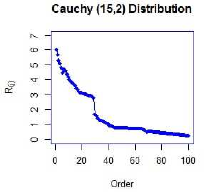
Figure 4: Ordered values of the statistic $R_{j}$. The largest 100 are shown.

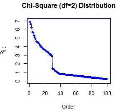
Figure 5: Ordered values of the statistic $R_{j}$. The largest 100 are shown.

3.2 Simulated Datasets

We also simulate a large number of datasets with different configurations to evaluate our approach. In general, in each simulation run 1000 protein markers are generated, and the expression profiles of each protein are simulated according to the following steps. Note that the parameters we use are the estimated values of those from the data sets acquired and processed by OpenSWATH [Röst et al., 2014], where proteins were under the matrices of water and human. Water is the simplest matrix among them, with clean signals, whereas human is the most complex under considerable interference. Simulated data points are denoted as $X^{i}_{kj}$, which is the expression intensity for the $j-$th protein of the $k-$th subject within the $i-$th condition. An example of simulated data layout is shown in Table  1.

1. Step 1. Generate the expression intensity $X^{i}_{kj}$ according to the following equation ([Röst et al., 2014]).

   $$X^{i}_{kj}=\mu+C_{i}+S(C)_{k(i)}+F_{j}+\epsilon^{i}_{kj}$$

2. Step 2. In the equation above $C_{i}$ stands for the main effect of a condition, $S(C)_{k(i)}$ the effect of each subject within a condition, and $F_{j}$ the main effect of each protein. We then generate the source of variations for the true markers and plain markers as follows. We simulate 2 conditions, $i=1,2$.

   For true markers $C_{1}\neq C_{2}$. For plain markers $C_{1}=C_{2}$. Then the other items in the above equation are simulated for normal distributions as follows.

   $$S(C)_{k(i)}\sim N(0,\sigma^{2}_{S}),$$

   $$F_{j}\sim N(0,\sigma^{2}_{F}),$$

   $$\epsilon^{i}_{kj}\sim N(0,\sigma^{2}).$$

3. Step 3. Set the parameter values according to [Röst et al., 2014]. We have $\mu=15$, $\sigma^{2}_{S}=27.37$, and $\sigma^{2}_{F}=0.98$. The sample size for each condition and the number of proteins vary in different simulation runs. The error term $\epsilon^{i}_{kj}$’s variance depends on the matrices. We have $\sigma^{2}=2.23$ for human background, the most complex matrix; $\sigma^{2}=0.48$ for water background, the matrix with the smallest level of interference.

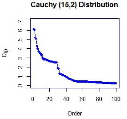
Figure 6: Ordered values of the statistic $D_{j}$. The largest 100 are shown.

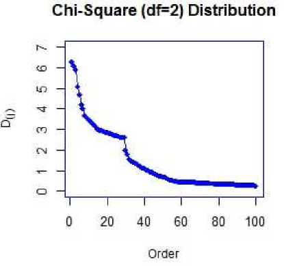
Figure 7: Ordered values of the statistic $D_{j}$. The largest 100 are shown.

3.3 Robust Performance Against Deviations from Normality

Although the two statistics in Section 2.1 are constructed as a ratio of a mixture distribution or the empirical distribution versus a pooled univariate normal, they show robust performance with non-normal distributions too. Figure 2 shows the empirical expression profile distributions of plain markers in HRM data. The most important feature of plain markers is that their expression profile distributions are unimodal. Hence the fundamental idea behind our approach is to separate bimodal distributions from unimodal distributions, which lead to accurate identification of true markers. The underlying actual distributions do not need to strictly follow normality assumptions for our approach to perform well. Here we demonstrate the robust performance of the two statistics against strong deviations from normality.

In one experiment, we have 10 samples per condition. We simulate 1000 proteins as specified in Section 3.2 but with different error term distributions, where there are 30 true markers and 970 plain markers. The error terms are simulated according to Cauchy distribution with location parameter 15 and scale parameter 2 (Figure 4) and chi-square distribution with two degrees of freedom (Figure 5). Cauchy distribution has much heavier tails than normal and chi-square with two degrees of freedom is very skewed distribution. Plain markers have $C_{1}=C_{2}=U$ where $U$ is randomly sampled following a uniform distribution over $[1,100]$. The effect size is 3 fold for true markers. The fold change is defined on log base 2 scale. True markers have $C_{1}=\log_{2}(6)+U$ and $C_{2}=\log_{2}(2)+U$ where $U$ is randomly sampled from a uniform distribution over $[1,10]$. The resulting expression profile distributions for both plain markers and true markers are strongly non-normal.

The proteins are ordered by their $R_{j}$ values. The largest 100 proteins are shown in Figures 4 and  5. The ordered values of the statistic $R_{j}$, which works well for not-too-small sample size, show a sudden drop after the largest values. We choose the cutoff for $R_{j}$ at where the drop occurs. This pattern is also observed from the two experimental datasets in Section 3.4. We select the markers with $R_{j}$ values larger than the cutoff. Based on this selection method, we are able to accurately identify 1) the number of truly relevant markers; 2) the relevant markers themselves.

In another experiment we simulate 1000 proteins as in the first experiment, only there are 3 samples per conditions. The statistic $D_{j}$ for very small sample size is used. Figures 6 and 7 show the order values of $D_{j}$, the 100 largest ones, which exhibit the same pattern. With very small sample size, we are still able to accurately identify the relevant markers.

3.4 High Sensitivity and Low FDR

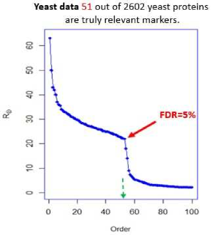
Figure 8: Ordered values of the statistic $R_{j}$ for Yeast Data. The largest 100 are shown.

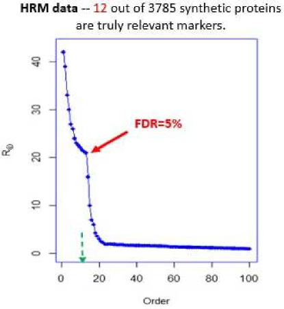
Figure 9: Ordered values of the statistic $R_{j}$ for HM Data. The largest 100 are shown.

Table 3: Sensitivity and empirical FDR for Yeast and HRM data

	HRM data		Yeast data
	Sensitivity	Empirical FDR	Sensitivity	Empirical FDR
LIMMA	$\frac{12}{12}=1.00$	$\frac{14}{26}=0.54$	$\frac{51}{51}=1.00$	$\frac{36}{87}=0.41$
RP	$\frac{12}{12}=1.00$	$\frac{9}{21}=0.43$	$\frac{48}{51}=0.94$	$\frac{31}{82}=0.38$
SAM	$\frac{12}{12}=1.00$	$\frac{8}{20}=0.40$	$\frac{50}{51}=0.94$	$\frac{41}{91}=0.45$
t-test	$\frac{12}{12}=1.00$	$\frac{16}{28}=0.57$	$\frac{50}{51}=0.98$	$\frac{55}{106}=0.52$
PCA	$\frac{6}{12}=0.50$	$\frac{1}{6}=0.17$	$\frac{8}{51}=0.16$	$\frac{1}{8}=0.13$
PLR	$\frac{3}{12}=0.25$	$\frac{0}{3}=0$	$\frac{6}{51}=0.12$	$\frac{0}{6}=0$
PLS-DA	$\frac{7}{12}=0.58$	$\frac{0}{7}=0$	$\frac{11}{51}=0.22$	$\frac{1}{12}=0.08$
SVM	$\frac{7}{12}=0.58$	$\frac{0}{8}=0$	$\frac{15}{51}=0.29$	$\frac{1}{16}=0.06$
Our $R_{j}$	$\frac{12}{12}=1.00$	$\frac{1}{13}=0.08$	$\frac{50}{51}=0.98$	$\frac{4}{54}=0.07$

We apply the statistic $R_{j}$ to the two experimental datasets, Yeast data and HRM data as discussed earlier. Figures 8 and 9 show the ordered values of $R_{j}$. Again we observe a sudden drop of $R_{j}$ values. We set the cutoff of $R_{j}$ to be 2.5. We then select the proteins that have $R_{j}$ values larger than cutoff. In Table 3 we compare the commonly used univariate and multivariate methods with our statistic $R_{j}$ based on sensitivity and FDR. For univariate methods FDR cutoff is set at 0.05, while for multivariate methods the algorithms stop based on their default stopping criteria. The univariate methods select too many markers, and suffer from high empirical FDR. The multivariate methods have strong model structures. They do not need all the relevant markers to achieve high classification accuracy. Hence they select too few markers, leading to very low sensitivity. Our approach, to cut off at where $R_{j}$ values suddenly drop, returns superior sensitivity with very low FDR.

Next we compare our approach with the commonly used methods in simulation studies. In a single run we simulate 1000 proteins as specified in Section 3.2 with the error terms normally distributed, where there are 30 true markers and 970 plain markers. Again plain markers have $C_{1}=C_{2}=U$ where $U$ is randomly sampled following a uniform distribution over $[1,100]$. The effect size is 3 fold for true markers. True markers have $C_{1}=\log_{2}(6)+U$ and $C_{2}=\log_{2}(2)+U$ where $U$ is randomly sampled following a uniform distribution over $[1,10]$. In one experiment we have 10 samples per condition and conduct 50 runs, with the average sensitivity and the average FDR shown in Table 4. In another experiment we have 3 samples per condition and conduct 50 runs, with the average sensitivity and the average FDR shown in Table 5.

Table 4: Average sensitivity and empirical FDR for water, human, yeast background with 10 samples per condition. FDR is set at 0.05 for univariate methods. $R_{j}$ cutoff is 2.5

	Water		Human
	Sensitivity	Empirical FDR	Sensitivity	Empirical FDR
LIMMA	$0.87$	$0.50$	$0.67$	$0.40$
RP	$0.73$	$0.41$	$0.80$	$0.33$
SAM	$0.90$	$0.44$	$0.77$	$0.43$
t-test	$0.70$	$0.29$	$0.50$	$0.40$
PCA	$0.17$	$0.20$	$0.13$	$0.25$
PLR	$0.40$	$0.25$	$0.33$	$0.1$
PLS-DA	$0.23$	$0.29$	$0.13$	$0.04$
SVM	$0.40$	$0.17$	$0.37$	$0.09$
Our $R_{j}$	$0.90$	$0.15$	$0.77$	$0.17$

Table 5: Average sensitivity and empirical FDR for water, human, yeast background with 3 samples per condition. FDR is set at 0.1 for univariate methods. $D_{j}$ cutoff is 2.5

	Water		Human
	Sensitivity	Empirical FDR	Sensitivity	Empirical FDR
LIMMA	$0.40$	$0.54$	$0.48$	$0.51$
RP	$0.53$	$0.43$	$0.55$	$0.58$
SAM	$0.37$	$0.40$	$0.40$	$0.40$
t-test	$0.23$	$0.57$	$0.43$	$0.41$
PCA	$0.37$	$0.37$	$0.19$	$0.13$
PLR	$0.30$	$0.13$	$0.13$	$0.16$
PLS-DA	$0.41$	$0.09$	$0.38$	$0.40$
SVM	$0.50$	$0.25$	$0.45$	$0.35$
Our $D_{j}$	$0.67$	$0.20$	$0.53$	$0.31$

4 Conclusion and Discussion

Our approach is superior to the popularly applied methods univariate and multivariate methods given reasonable sample size. Our approach shows good performance for very small sample size, especially under water background. In addition, we notice that nowadays most of the experimental designs have allowed us to merge samples from adjacent conditions (groups). At the end of the day we may not have to rely on the alternative procedure for very small sample size cases.

Meanwhile, as the primary goal of this paper is to accurately identify relevant biomarkers in discovery study, which is mostly balanced design with moderate or small sample size, the method we propose is mainly for the balanced design given two conditions. Thus how to handle the data acquired from highly unbalanced design under multiple conditions (more than two) with potentially very small sample size for certain conditions is part of our future work.

The nature of discovery study combined with the advancement of DIA experiment result in sparse and high dimensional data. It is known that popular univariate methods struggle under sparsity and multivariate methods stumble under high dimensionality.

Nonetheless, our proposed likelihood-based statistic resolves the problem from a critical perspective – accurately estimates the number of truly relevant markers. This feature can effectively resolves the aforesaid drawbacks from current methods.

From multiple experimental and simulated data sets we demonstrate that our approach is able to accurately identify the set of truly relevant protein markers. The implication is that our proposed method can simplify the unnecessarily lengthy and costly process of biomarker discovery without compromising the findings of markers correlating with conditions.

References

- [Rifai et al., 2006] Rifai, N., Gillette, M.A. and Carr, S.A., 2006. Protein biomarker discovery and validation: the long and uncertain path to clinical utility, Nature biotechnology, 24(8), 971-983.
- [Pandey et al., 2000] Pandey, A. and Mann, M., 2000. Proteomics to study genes and genomes. Nature, 405(6788), 837-846.
- [Carvalho et al., 2010] Carvalho, P.C., Han, X., Xu, T., Cociorva, D., Carvalho, M.D.G., Barbosa, V.C. and Yates III, J.R., 2010. XDIA: improving on the label-free data-independent analysis. Bioinformatics, 26(6), 847-848.
- [Gillet et al., 2012] Gillet, L.C., Navarro, P., Tate, S., Röst, H., Selevsek, N., Reiter, L., Bonner, R. and Aebersold, R., 2012. Targeted data extraction of the MS/MS spectra generated by data-independent acquisition: a new concept for consistent and accurate proteome analysis. Molecular & Cellular Proteomics, 11(6), O111-016717.
- [Smyth, 2004] Smyth, G. K., 2004. Linear models and empirical bayes methods for assessing differential expression in microarray experiments. Stat Appl Genet Mol Biol, 3(1), 3.
- [Tusher et al., 2001] Tusher, V.G., Tibshirani, R. and Chu, G., 2001. Significance analysis of microarrays applied to the ionizing radiation response. Proceedings of the National Academy of Sciences, 98(9), 5116-5121.
- [Breitling et al., 2004] Breitling, R., Armengaud, P., Amtmann, A. and Herzyk, P., 2004. Rank products: a simple, yet powerful, new method to detect differentially regulated genes in replicated microarray experiments. FEBS letters, 573(1-3), 83-92
- [Bruderer et al., 2015] Bruderer, R., Bernhardt, O.M., Gandhi, T., Miladinović, S.M., Cheng, L.Y., Messner, S., Ehrenberger, T., Zanotelli, V., Butscheid, Y., Escher, C. and Vitek, O., 2015. Extending the limits of quantitative proteome profiling with data-independent acquisition and application to acetaminophen-treated three-dimensional liver microtissues. Molecular & Cellular Proteomics, 14(5), 1400-1410.
- [Selevsek et al., 2015] Selevsek, N., Chang, C.Y., Gillet, L.C., Navarro, P., Bernhardt, O.M., Reiter, L., Cheng, L.Y., Vitek, O. and Aebersold, R., 2015. Reproducible and consistent quantification of the Saccharomyces cerevisiae proteome by SWATH-mass spectrometry. Molecular & Cellular Proteomics, 14(3), 739-749.
- [Röst et al., 2014] Röst, H.L., Rosenberger, G., Navarro, P., Gillet, L., Miladinović, S.M., Schubert, O.T., Wolski, W., Collins, B.C., Malmström, J., Malmström, L. and Aebersold, R., 2014. OpenSWATH enables automated, targeted analysis of data-independent acquisition MS data. Nature biotechnology, 32(3), 219-223.
- [Bilmes, 1998] Bilmes, J.A., 1998. A gentle tutorial of the EM algorithm and its application to parameter estimation for Gaussian mixture and hidden Markov models. International Computer Science Institute, 4(510), 126.
- [Massey Jr, 1951] Massey Jr, F. J., 1951. The Kolmogorov-Smirnov test for goodness of fit. Journal of the American statistical Association, 46(253), 68-78.
- [Lilliefors, 1967] Lilliefors, H. W., 1967. On the Kolmogorov-Smirnov test for normality with mean and variance unknown. Journal of the American statistical Association, 62(318), 399-402.